Abstract— Dental radiographs are essential in diagnosing the pathology of the jaw. However, similar radiographic appearance of jaw lesions causes difficulties in differentiating cyst from tumor. Therefore, we conducted a development of computer-aided classification system for cyst and tumor lesions in dental panoramic images. The proposed system consists of feature extraction based on texture using the first-order statistics texture (FO), Gray Level Co-occurrence Matrix (GLCM) and Gray Level Run Length Matrix (GLRLM). In this work, there were thirty three features which were classified using Support Vector Machine (SVM) based classification. The result shows that differentiation of cyst from tumor lesions can achieve accuracy up to 87.18% and Area Under the Receiver Operating Characteristic (AUC) curve up to 0.9444. When using the number of features used as predictors, the highest accuracy obtained were 8462% using FO, 61.54% using GLCM, 76.92% using GLRLM, 84.62% using the combination of FO and GLCM, 87.18% using the combination of FO and GLRLM, 75.56% using the combination of GLCM and GLRLM, and 87.18% using the combination of FO, GLCM and GLRLM. The highest AUC value was 0.9361 using FO, using GLCM was 0.8667, using GLRLM was 0.8722, using the combination of FO and GLCM was 0.9278, using the combination of FO and GLRLM was 0.9444, using the combination of GLCM and GLRLM was 0.8417, and using the combination of FO, GLCM and GLRLM was 0.9278. Based on the AUC value, the level of accuracy of this prediction can be categorized as ‘Excellent’.
Index Terms— cyst and tumor lesion, dental panoramic images, FO, GLCM, GLRLM, SVM
I. INTRODUCTION
A variety of disorders can be found in human jawbone. These disorders consist of various types of cyst and tumor lesions that have been clinically classified [1]–[6].
Some of these lesions (e.g. a malignant tumor lesion)
Manuscript received June 26th, 2012; revised September 17th, 2012,second revised November 16th 2012.
Ingrid Nurtanio is with Electrical Engineering Department, Hasanuddin University, Makassar, 90245, Indonesia (phone number : +62-8152522716; e-mail : [email protected]).
Eha Renwi Astuti is with Dentistry Department, Airlangga University, Surabaya, Indonesia. Email : [email protected]
I Ketut Eddy Purnama is with Electrical Engineering Department, Institut Teknologi Sepuluh Nopember, Surabaya Indonesia, Email : [email protected]
Mochamad Hariadi is with Electrical Engineering Department, Institut Teknologi Sepuluh Nopember, Surabaya, Indonesia. Email: [email protected]
Mauridhi Hery Purnomo is with Electrical Engineering Department, Institut Teknologi Sepuluh Nopember, Surabaya, Indonesia. Email: [email protected]
have a potential to develop into cancer. Thus, early detection of this malignant lesion can considerably reduce morbidity and mortality. Lesion appearance of the visual part of dental panoramic images determines the future treatment of the patient. Therefore by knowing the features of lesions and extracting the difference between them, the classification can be immediately conducted and evaluated [7]–[10]. Previously, medical experts evaluated the classification of the lesions by doing manual segmentation and they generally agreed on the position of the lesion boundaries in the recorded images. As machinery, after supervised learning, is generally more efficient than humans in differentiating oral diseases, we proposed a computer-aided classification. However, lesion classification is still a challenging problem for computer vision due to the variability of the shape and appearance of cyst and tumor lesions.
Currently our image database includes cases of two types of lesions, the cyst lesions and the tumor lesions. Both types of lesions typically have a smooth, round or oval periphery [4], [6] and are not easily differentiated, see Fig. 1. This situation makes a dentist unable to determine exactly whether it is a tumor or a cyst.
Research to differentiate cyst from tumor using computer-aided classification has never been conducted yet. The most
Classifying Cyst and Tumor Lesion Using
Support Vector Machine Based on Dental
Panoramic Images Texture Features
Ingrid Nurtanio,
Member, IAENG
, Eha Renwi Astuti, I Ketut Eddy Purnama, Mochamad Hariadi,
Mauridhi Hery Purnomo
(a)
(b)
relevant recent research was about the Application to Oral Lesion Detection in Color Images Using Active Contour Models [11]. To fill in the gap, we conducted a research to distinguish cyst from tumor lesion using Support Vector Machines (SVMs) based on texture features. Texture is one of the crucial characteristics used to identify objects or region of interest in an image.
Various research based on textures have been reported [12]– [19] but the object of research were not in the field of dental panoramic images and the classifier was not SVM. Recently we have used the Gray Level Co-occurrence Matrix (GLCM) texture features to differentiate cyst from tumor lesions [8], but the accuracy value was only 63.33%. Thus, in this paper we propose a novel approach involving an automatic assessment using of the first-order statistics texture (FO), GLCM and Gray Level Run Length Matrix (GLRLM) to extract the features of cyst and tumor lesions.
This paper is organized as follows: Section 2 consists of the materials and methods concerning FO, GLCM, GLRLM and SVM. Section 3 presents the experimental result about the feature extraction and the classification and the computation of AUC from ROC curve to measure SVMs classifier performance. Section 4, discusses the result and section 5 contains the conclusions.
II.MATERIALSANDMETHODS
A.Materials
A dataset of 133 dental panoramic images was prepared to cover various types of cyst lesions (radicular cyst, dentigerous cyst, buccal bifurcation cyst, keratocyst, calcifying odontogenic cyst, nasopalatine cyst, simple bone cyst) and various types of tumor lesions (ameloblastoma, ameloblastic fibroma, adenomatoid odontogenic tumor, odontoma, cementoblastoma, torus palatinus, torus mandibularis, exostosis, enostosis, myxoma, osteoma, hemangioma, osteoid osteoma, osteo blastoma) derived from Oral Radiology [4] and Cranex 2.5+ Soredex dental panoramic x-Ray Machine model PT-12SA. All images were already in digital forms. The total images of the cyst lesions were 53 images and those for the tumor lesions were 80 images. The position of the cyst and tumor regions was provided by an experienced radiologist acting as the co-author of this paper.
B.Methods
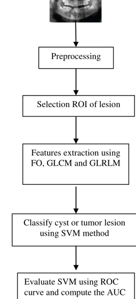
In this paper, we develop methods to classify cyst and tumor lesions using the properties of dental panoramic images. The stage of the cyst and tumor lesion classification methods is presented in Fig. 2.
B.1. Preprocessing
As dental panoramic images are not easy to interpret, preprocessing is viewed as necessity to improve the quality of the images. This stage leads to a less complicated and more reliable feature extraction phases [16]. The preprocessing procedure transforms color images to gray images by normalizing the values of the pixels with respect to the length of the gray scale. In this work, the Gaussian filter was used to remove noise and hence smooth the images which can then improve the contrast of dental panoramic images.
Fig. 2. Stage of the cyst and tumor lesion classification method
Fig. 3. The image after preprocessing
Fig. 3 represents the image after preprocessing stage.
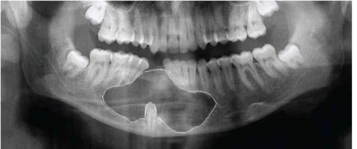
B.2. Selection of Region of Interest (ROI)
ROI is a region used to extract features. In this research the ROIs were the cyst and tumor lesions on the dental panoramic images. All lesions were manually selected from the images by a well-trained operator and further confirmed by a radiologist. A ROI of size 40 40 pixels was extracted with mass centered in the window. Then the masses were divided into two sets: the learning set and the testing set. Using one three hold out cross validation, the learning set was composed of 38 cyst images and 56 tumor images while the testing set contained 15 cyst images and 24 tumor images. Fig. 4 represents the ROI of an image. Fig. 5 represents the cyst and tumor lesions after cropping the ROI into 40 40 pixels.
Preprocessing
Selection ROI of lesion
Features extraction using FO, GLCM and GLRLM
Classify cyst or tumor lesion using SVM method
Fig. 4. The selected ROI of image
(a) (b)
Fig. 5. (a) The ROI of Cyst Lesion and (b) the ROI of Tumor Lesion
B.3. Feature Extraction
The features were extracted using statistical texture analysis. Texture features were computed on the basis of statistical distribution of pixel intensity at a given position relative to other pixels in the matrix of the represented image. Depending on the number of pixels or dots in each combination, we utilized the first-order statistics, second-order statistics or higher-order statistics. The first-order statistics texture measures were statistically calculated from the original image values, such as the variance, without considering its relationships with the neighboring pixel. The second order measures considered the relationship between groups of two (usually neighboring) pixels in the original image. The third and higher order textures (considering the relationships among three or more pixels) were theoretically possible but not commonly implemented due to longer calculation time and interpretation difficulties. The feature extraction based on gray level co-occurrence matrix (GLCM) is the second order statistics that can be used to analyze images as a texture. For the higher-order statistics we used gray level run length matrix (GLRLM) to analyze the images. In this particular stage, we examined a set of 33 features that were applied to the ROI, 6 features from FO, 20 features from GLCM and 7 features from GLRLM.
B.3.1. FO (The first-order statistics texture)
An approach based on the statistical properties of the intensity of histogram is frequently used in texture analysis [12]. The features from FO are mean, standard deviation, smoothness, third moment, uniformity and entropy. If z is a random variable indicating intensity,
p(z) is the histogram of the intensity levels in a region, L
is the number of possible intensity levels, and we then computed the features using Eqs. (1-6).
Mean is a measure of average intensity:
) (
1
0
L
i
i ip z
z
m (1)
Standard deviation is a measure of average contrast:
1
0
2
) ( ) (
L
i
i
i m p z
z
(2)
Smoothness measures the relative smoothness of the intensity in a region:
2
1 1 1
R (3) Third moment measures the skewness of a histogram:
) ( )
( 3
1
0
3 i
L
i
i m p z
z
(4)
Uniformity, this measure is maximum when all gray levels are equal (maximally uniform) and decreases from there:
) (
1
0 2
i L
i
z p
U
(5)
Entropy is a measure of randomness:
) ( log )
( 2
1
0
i L
i
i p z
z p
e
(6)
B.3.2. GLCM (Gray Level Co-occurrence Matrix)
GLCM (also called gray tone spatial dependency matrix) is a tabulation of the frequencies or how often different combinations of pixel brightness values (gray levels) occur in an image [13]. GLCM texture indicates the relation between two pixels at a time, the reference and the neighbor pixel. Figure 6 represents the formation of the GLCM of the gray level (4 levels) image at the distance d = 1 and the direction of 0. There are two occurrences of pixel intensity 0 and pixel intensity 1 as neighbors (in the horizontal direction or the direction of 0). Therefore, the GLCM formed (Fig. 6(b)) value 2 in row 0, column 1. In the same way, GLCM row 1 column 1 is also given a value of 4, because there are four occurrences in which pixels with value 1 has pixels 1 as its neighbor (horizontal direction). As a result, the pixel matrix represented in Fig. 6(a) can be transformed into GLCM as Fig. 6(b).
(a) (b)
Fig. 6 (a) Example of an image with 4 gray level image. (b) GLCM for distance 1 and direction 0
0 0 1 1 1
0 0 1 1 1
0 2 2 2 2
2 2 3 3 3
2 2 3 3 3
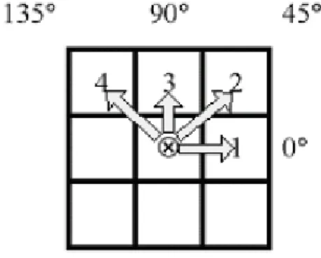
Fig. 7. Direction of GLCM generation. From the center () to the pixel 1 representing direction = 0 with distance d = 1, to the pixel 2 direction = 45 with distance d =1, to the pixel 3 direction = 90 with distance d = 1, and to the pixel 4 direction = 135 with distance d =1.
In addition to the horizontal direction (0), GLCM can also be formed for the direction of 45, 90, and 135 as shown in Fig. 7.
Prior to the calculation, the texture measures require that each GLCM cell contains a probability. This process is called normalizing the matrix. Normalization involves division by the sum of values. Normalization equation is:
1 0 , ) , ( ) , ( ) , ( N j i j i V j i V j ip (7)
where i is the row number and j is the column number. Haralick and his colleagues [13] extracted 14 features from the co-occurrence matrix, but in this research we used only 5 features, i.e. contrast, correlation, energy, homogeneity, and entropy with 4 direction and distance
d=1.
The features we considered were:
) , ( ) ( 1 0 ,
2pi j j i Contrast N j i
(8)
1 0 , 2 1 0 , 2 1 0 , 1 0 , 1 0 , ) )( , ( ) )( , ( )) , ( ( )) , ( ( ) , ( ) )( ( N j i j j N j i i i N j i j N j i i N ji i j
j i j j i p i j i p j i p j j i p i where j i p j i n Correlatio (9)
1 0 , 2 ) , ( N j i j i pEnergy (10)
1 0 , 2 ) ( 1 ) , ( N ji i j
j i p y
Homogeneit (11)
1 0 , )) , ( ln )( , ( N j i j i p j i pEntropy (12)
B.3.3. Gray Level Run Length Matrix (GLRLM)
GLRLM is a matrix from which the texture features can be extracted for texture analysis. A texture is understood as a pattern of gray intensity pixel in a particular direction from the reference pixels. Run length is the number of the adjacent pixels that have the same gray intensity in a particular direction. Gray level run length matrix is a two dimensional matrix where each element p(i,j) is the number of elements j with the intensity i, in the direction . Figure 8(a) below shows a matrix of size 44 pixel image with 4 gray levels. Figure 8(b) is the representation matrix GLRL (Gray Level Run Length) in the direction of 0 [p(i,j =0)]. In addition to the 0 direction, GLRL matrix can also be formed in the other direction, i.e. 45, 90 or 135 (see fig. 9). Some texture features can be extracted from the GLRL matrix, such as Short Runs Emphasis (SRE), Long Runs Emphasis (LRE), Gray Level Non-uniformity (GLN), Run Percentage (RP), Run Length Non-uniformity (RLN), Low Gray Level Run Emphasis (LGRE), and High Gray Level Run Emphasis (HGRE).
The feature can be defined as follows in Eqs. (13-19):
M i N j r j j i p n SRE 1 1 2 ) , ( 1 (13)
M i N j r j j i p n LRE 1 1 2 ) , ( 1 (14)(a) (b) Fig. 8. (a) Matrix of image 4 x 4 pixels. (b) GLRL Matrix.
Fig. 9. Run Direction 1 2 3 4
1 3 4 4 3 2 2 2 4 1 4 1
Gray level Run length (j)
i 1 2 3 4
1 4 0 0 0
2 1 0 1 0
3 3 0 0 0
2 1 1 ) , ( 1
M i N j r j i p nGLN (15)
j j i p n RP r * ) , (
(16)
2
1 1
) , (
1
N j M i r j i p n
RLN (17)
M i N j r i j i p n LGRE 1 1 2 ) , ( 1 (18)
M i N j r i j i p n HGRE 1 1 2 ) , ( 1 (19) B.4. ClassificationAfter the extraction and selection, the features were input into classifier to categorize the images into the cyst or tumor lesions. We used the Support Vector Machine (SVM) method to categorize these lesions.
B.4.1. Support Vector Machine (SVM) Classifiers
SVM is a state-of-the-art classification method introduced by Boser, Guyon & Vapnik in 1992 [20] for a binary classification. From what originally developed for binary classification problems, the key concept of SVMs is development into the use hyper-planes to define decision boundaries to separate data points of different classes. This makes SVMs able to handle both of separable and non-separable cases in simple (linear) classification tasks, as well as more complex (nonlinear), classification problems. The idea behind SVMs is to map the original data points from the input space to a high dimensional feature space, or even infinite-dimensional feature space to simplify the classification problem. The mapping can be done by choosing a suitable kernel function. To map the input data into a higher dimension space where they are supposed to have a better distribution, kernel functions are implemented. Then, an optimal separating hyper-plane in the high dimensional feature space is chosen [7].
Consider a training data set {xi,yi}, with xi d being the input vectors and yi {-1,+1} the class labels.
Fig. 10. SVMs allow mapping of the data from the input space to a high-dimensional feature space [21].
SVMs map the d-dimensional input vector x from the input space to the d1-dimensional feature space using a (non)linear function (.) : dd1. The separating hyper-plane in the feature space is then defined as WT(x) + b = 0, with b and W an unknown vector with the same dimension as (x). A data point x is assigned to the first class if f(x) = sign(WT (x) + b) equals +1 or to the second class if f(x) equals -1.
However, in our study, there were some overlapping values between the data in both classes, thus a perfect linear separation was impossible to conduct. Therefore, a restricted number of misclassification should be tolerated around the margin. The resulting optimization problem for SVMs, where the violation of the constraints is penalized, was written as: , ., ,... 1 , 0 1 ) ) ( ( subject to 2 1 min 1 , , N i b x W y C W W i i i T i N i i T b W
(20)where C is a positive regularization constant. The trade-off between a large margin and misclassification error were defined by the regulation constant in the cost function. For non-separable data, an upper bound of the misclassification error was controlled using slack variable () by the soft-margin SVM. The value of i indicated the distance of xi with respect to the decision boundary. Equivalently, Lagrangian with Lagrange multipliers i 0 for the first set of constraints can be used to write the optimization problem for SVMs in the dual space. By solving a quadratic programming problem, the solution for the Lagrange multiplier can be obtained. Finally, the SVM classifier takes the form:
SV i i iiyK x x b
sign x f # 1 ) , ( )
( (21) where #SV represents the number of support vectors and the kernel function K(.,.) is positively definite.
Furthermore, K(x,xi) (x)T(x) is called the kernel function. In the optimization problem only K(.,.) which is related to (.) is used. This enables SVMs to work in a high-dimensional (or infinite-high-dimensional) feature space, without actually performing calculations in this space. We used Gaussian Kernel in this study with kernel function being:
2 2 2 exp ) , ( i i x x x x
K (22) where is the kernel parameter.
B.5. Evaluation
In this research, we employed the receiver operating characteristic (ROC) curve because of its comprehensive and fair evaluation ability [7]. A ROC curve is the plotting of true positive fraction (TPF) as the function of false positive fraction (FPF) [22], [23]. The area under the ROC curve (AUC) can be used as a criterion. Table I shows the classifying level of accuracy based on AUC [16].
TABLE I
CLASSIFYING LEVEL OF ACCURACY BASED ON AUC [16]
AUC value Classified as
0.90 – 1.00 Excellent 0.80 – 0.90 Good
0.70 - 0.80 Fair 0.60 – 0.70 Poor 0.50 – 0.60 Failed
FN FP TN TP
TN TP accuracy
(23)
FP TN
TN y specificit
(24)
FN TP
TP y
sensitivit
(25)
where TP is the number of true positives, TN is the number of true negatives, FP is the number of false positives and FN is the number of false negatives.
III. EXPERIMENTS AND RESULTS
All the experiments were conducted in Matlab Ver 7.1 running on a PC Intel-Pentium Centrino with RAM 1 GB. A total of 53 cyst lesions and 80 tumor lesions measuring 4040 pixels were transformed into FO, GLCM and GLRLM. Six texture features were extracted based on FO, 20 texture features were extracted based on GLCM, 7 texture features were extracted based on GLRLM. The 6 features from FO were mean, standard deviation, smoothness, third moment, uniformity and entropy.
Table II shows the feature values extracted from FO for both lesions in Fig. 5. It is obvious that the values of the features from both classes are overlapping, but the minimum and maximum values for both classes are different. This result indicate that the classification process cannot be easily done (not linear) because of the overlapping value. However, the maximum and minimum feature values in each class make the classification still possible to conduct (non linear classification). For example, the mean values of cyst lesion are from 13.7650 until 213.2888 while the mean values of tumor lesion are from 85.0038 until 252.3044. This means distinguishing the cyst lesions from the tumor ones is now possible using SVM.
TABLE II
TABULATED MINIMUM AND MAXIMUM FEATURE VALUES FOR CYST AND TUMOR CLASSIFICATION EXTRACTED FROM
FIRST-ORDER STATISTICS TEXTURE
Features Cyst Lesions Tumor Lesions
Min. Max. Min. Max.
Mean 13.7650 213.2888 85.0038 252.3044 Standard deviation 0.5163 3.3309 0.4383 3.6734 Smoothness 0.8377 0.9709 0.8142 0.9735 Third moment -0.0334 0.2369 -0.6272 0.2748 Uniformity 0.0110 0.1246 0.0086 0.4602 Entropy 4.2028 6.7591 2.4005 7.0271
TABLE III
TABULATED MINIMUM AND MAXIMUM FEATURE VALUES FOR CYST AND TUMOR CLASSIFICATION EXTRACTED FROM GLC M
Features Cyst Lesion Tumor Lesion
Min. Max. Min. Max.
Direction = 00, Distance = 1
Contrast 0.1205 2.8718 0.1365 2.8603 Correlation -0.2779 0.9888 -0.2903 0.9653 Energy 0.0527 0.4895 0.0706 0.7107 Homogeneity 0.5730 0.9397 0.6090 0.9377 Entropy 0.0000 1.8815 0.0000 1.7850 Direction = 450, Distance = 1
Contrast 0.2249 2.2715 0.1644 1.9244 Correlation 0.2610 0.9741 0.2457 0.9391 Energy 0.0498 0.4670 0.0616 0.7251 Homogeneity 0.5518 0.8927 0.6037 0.9424 Entropy 0.0687 2.0012 0.0048 1.8431 Direction = 900, Distance = 1
Contrast 0.1673 2.6532 0.1353 2.6551 Correlation -0.2247 0.9842 -0.2566 0.9550 Energy 0.0602 0.4771 0.0714 0.7085 Homogeneity 0.5922 0.9181 0.6177 0.9450 Entropy 0.0000 1.9115 0.0047 1.6324 Direction = 1350, Distance = 1
Contrast 0.1795 2.3064 0.2163 1.8725 Correlation 0.2499 0.9860 0.2186 0.9464 Energy 0.0491 0.4632 0.0626 0.7185 Homogeneity 0.5573 0.9103 0.6085 0.9349 Entropy 0.0583 1.9983 0.0202 1.8378
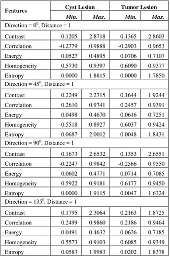
There were 20 features from GLCM which were originated from contrast, correlation, energy, homogeneity and entropy, of four directions (0, 45, 90, and 135) and distance = 1 as shown in Table III.
Similar to previous results, the feature values in Table III are also overlapping, but the minimum and the maximum values between these two classes are different except for the entropy. The minimum entropy value at direction 0 in Table III is 0.0000 on both of lesions leading to a low accuracy in the value of feature extraction (61.54%).
The seven features of GLRLM were: SRE (Short Runs Emphasis), LRE (Long Runs Emphasis), GLN (Gray Level Non-uniformity), RP (Run Percentage), RLN (Run Length Non-uniformity), LGRE (Low Gray Level Run Emphasis), and HGRE (High Gray Level Run Emphasis).
TABLE IV
TABULATED MINIMUM AND MAXIMUM FEATURE VALUES EXTRACTED FROM GLRLM AT DIRECTION= 0
Features Cyst Lesion Tumor Lesion
Min. Max. Min. Max.
Table IV shows feature values extracted from GLRLM for both lesions in Fig. 5. Like Table II and III, the feature values at table IV is also overlapping, but the minimum and maximum values of the two classes are different. This means that the cyst lesions and tumor lesions can be distinguished using this feature values.
Tables II, III and IV show that there are some overlapping values between the data in both classes, and making a perfect linear separation cannot be performed. This problem was handled by SVMs in the nonlinear case. SVM maps the original data points from the input space to a high dimensional feature space (see Fig. 10). We use one third hold out cross validation of 133 data images by randomly selecting 94 images referring to each class as data training, while the rest (39 images) as the data test. The experiments were conducted 20 times. Using SVM with kernel Gaussian, C = 10000, alpha = 1e-7 and sigma = 4000, we obtained accuracy up to 87.18%, depending on the random observations which were used as a predictor. We obtained up to 84.62% accuracy using FO, 61.54% using GLCM, 76.92% using GLRLM, 84.62% using the combination of FO and GLCM, 87.18% using the combination of FO and GLRLM, 75.56% using the combination of GLCM and GLRLM, and 87.18% using the combination of FO, GLCM and GLRLM. Using ROC curve and computing the AUC, we obtain the AUC up to 0.9444. Using FO, we obtain the AUC up to 0.9361, 0.8667 for GLCM, 0.8722 for GLRLM, 0.9278 for the combination of FO and GLCM, 0.9444 for the combination of FO and GLRLM, 0.8417 for the combination of GLCM and GLRLM, and 0.9278 for the combination of FO, GLCM and GLRLM. Figure 11 shows the graphic of accuracy. Figure 12 shows the graphic of AUC values between each features group. And Fig. 13 shows the ROC curve for the combination of FO and GLRLM which is the highest classification rate (represented by solid bold line), the combination of GLCM and GLRLM which is the lowest classification rate (represented by solid line) and all combinations (represented by dash line). Table V shows the comparison of accuracy and AUC value for each feature group and their combinations. The bold values in table V are the highest performance achieved as the result of the combination of FO and GLRLM. The accuracy value achieved was 87.18% (as shown in Fig. 11) and the AUC value achieved was 0.9444 (as shown in Fig. 12).
TABLE V
COMPARISON ACCURACY AND AUC VALUE AMONG DIFFERENT TEXTURE FEATURES EXTRACTION
Texture Features Accuracy AUC
Min. Max. Min. Max.
First-order (FO) 64.10% 84.62% 0.7639 0.9361 GLCM 61.54% 61.54% 0.6472 0.8667 GLRLM 56.41% 76.92% 0.6278 0.8722 FO + GLCM 64.10% 84.62% 0.7556 0.9278 FO + GLRLM 66.67% 87.18% 0.7556 0.9444 GLCM + GLRLM 53.85% 75.56% 0.6444 0.8417 FO+GLCM+GLRLM 69.23% 87.18% 0.7278 0.9278 The values in bold typesare the highest performance.
Fig. 11. Graphic of the accuracy values between each features group. The highest accuracy is 87.18%, which is achieved from the combination of FO and GLRLM and the combination of FO, GLCM and GLRLM features method. GLCM feature method shows the lowest accuracy value of 61.54% .
Fig.12. Graphic of AUC values between each feature group. The highest AUC is 0.9444 from the combination of FO and GLRLM. The combinations of GLCM and GLRLM show the lowest AUC value of 0.8417
IV. DISCUSSIONS
In this study, we observed that the texture features can be used to classify cyst and tumor lesions.
Texture is one of the crucial characteristics used to identify objects or ROI in an image [13].
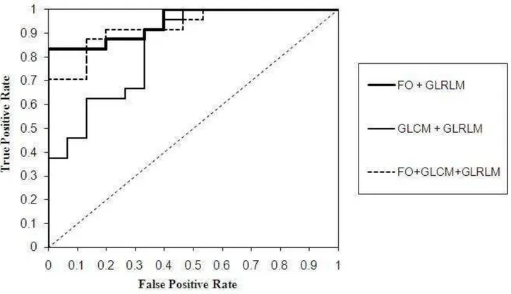
Fig. 13. ROC curve for the highest AUC value of 0.9444 was resulted from the combination of FO and GLRLM (solid bold line). Combination of GLCM and GLRLM get the lowest AUC value of 0.8417. The combination of all the methods used gets the AUC value of 0.9278 (dash line)
Tables II, III and IV show that there is an overlapping value between the feature data for cyst and the feature data for tumor. Thus, the linear classification is impossible to be implemented. SVM can be used to separate this data using the kernel function.
The result shows that choosing the kernel and its parameter is an important step to classify the features of lesion. In this study, we used Gaussian Kernel with C= 10000, alpha=1e-7, sigma = 4000 that yields the best result. The performance of accuracy evaluation by the statistical prediction model can also be done by using ROC curve analysis. ROC curve is a graphical plotting with the y-axis expressing sensitivity (true positive rate) and the x-axis expressing false positive rate [16], [17], [24]. Figure 13 of the ROC curve shows the discrimination among the combination of FO and GLRLM, the combination of FO, GLCM and GLRLM, and the combination of GLCM and GLRLM, as the predictors for the 4040 pixels image size. The overall classification of the accuracies and the AUC values are shown in table V. The combination of FO and GLRLM achieves 0.9444, FO achieves 0.9361, the combination of FO and GLCM achieves 0.9278, and the combination of FO, GLCM and GLRLM achieves 0.9278. Thus the four methods achieve the highest (excellent) classification rate (see Table I). While GLRLM, GLCM, the combination of GLCM and GLRLM, achieve the good classification rate of 0.8722, 0.8667 and 0.8417 respectively.
All methods achieve very good accuracy except for the GLCM (61.54%). This means that without GLCM and with only the combination of FO and GLRLM, we have achieved the very good accuracies of classification.
V.CONCLUSION
In this paper, we have succeeded to prove our claim that texture features based on first-order statistics texture, GLCM and GLRLM can be used to classify cyst and tumor lesions using SVM classification method.
The result achieved very good accuracy (87.18%) except for the GLCM (61.54%).
The performance evaluation metrics for SVM classification represents an excellent result with AUC which is 0.9278 for the combination of FO, GLCM and GLRLM, 0.9278 for the combination of FO and GLCM, 0.9361 for the FO, and 0.9444 for the combination of FO and GLRLM, while GLRLM, GLCM, the combination of GLCM and GLRLM, achieved the good classification rate of 0.8722, 0.8667 and 0.8417 respectively.
The combination of FO and GLRLM achieved the highest accuracies and AUC value of 87.18% and 0.9444 respectively. GLCM achieved the lowest accuracies value of 61.54% and the combination of GLCM and GLRLM achieves the lowest AUC value of 0.8417. That means GLCM feature can be disregarded for this research or a further research should be conducted to increase the accuracy of GLCM texture features.
REFERENCES
[1] S. J. Theodorou, D. J. Theodorou, and D. J. Sartoris, “Imaging characteristics of neoplasms and other lesions of the jawbones: Part 1. Odontogenic tumors and tumorlike lesions,” Clinical Imaging, vol. 31, no. 2, pp. 114–119, Mar. 2007.
[3] D. J. Theodorou, S. J. Theodorou, and D. J. Sartoris, “Primary non-odontogenic tumors of the jawbones: An overview of essential radiographic findings,” Clinical Imaging, vol. 27, no. 1, pp. 59–70, Jan. 2003.
[4] S. C. White and M. J. Pharoah, Oral Radiology: Principles and Interpretation. Elsevier Health Sciences, 2008.
[5] F. Pasler and H. Visser, Pocket Atlas of Dental Radiology. Thieme, 2007.
[6] Z. Neyaz, A. Gadodia, S. Gamanagatti, and S. Mukhopadhyay, “Radiographical approach to jaw lesions,” Singapore Med J, vol. 49, no. 2, pp. 165–176; quiz 177, Feb. 2008.
[7] H. D. Cheng, J. Shan, W. Ju, Y. Guo, and L. Zhang, “Automated breast cancer detection and classification using ultrasound images: A survey,” Pattern Recognition, vol. 43, no. 1, pp. 299–317, Jan. 2010. [8] C. V. Angkoso, I. Nurtanio, I. K. E. Purnama, and M. H. Purnomo,
“Texture Analysis for Cyst and Tumor Classification on Dental Panaramic Images,” presented at the Seminar on Intelligent Technology and Its Applications (SITIA), Surabaya, 2011, pp. 15–19. [9] Y. C. Li, D. L. Yu, and H. Y. Cheng, “Data Clustering Using Chaotic Particle Swarm Optimization,” IAENG International Journal of Computer Science, vol. 39, no. 2, May 2012.
[10] J. A. R. Quintana, M. I. C. Murguia, and J. F. C. Hinojos, “Artificial Neural Image Processing Applications: A Survey,” Engineering Letters, vol. 20, no. 1, Feb. 2012.
[11] G. Hamarneh, A. Chodorowski, and T. Gustavsson, “Active contour models: application to oral lesion detection in color images,” in 2000 IEEE International Conference on Systems, Man, and Cybernetics, 2000, vol. 4, pp. 2458 –2463 vol.4.
[12] R. C. Gonzalez, R. E. Woods, S. L. Eddins, “Digital Image Processing Using MATLAB,” Pearson Prentice Hall, 2004. ch. 11. [13] R. M. Haralick, K. Shanmugam, and I. Dinstein, “Textural Features
for Image Classification,” IEEE Transactions on Systems, Man and Cybernetics, vol. SMC-3, no. 6, pp. 610 –621, Nov. 1973.
[14] R. N. Sutton and E. L. Hall, “Texture Measures for Automatic Classification of Pulmonary Disease,” IEEE Transactions on Computers, vol. C-21, no. 7, pp. 667 – 676, Jul. 1972.
[15] R. Sivaramakrishna, K. A. Powell, M. L. Lieber, W. A. Chilcote, and R. Shekhar, “Texture analysis of lesions in breast ultrasound images,” Computerized Medical Imaging and Graphics, vol. 26, no. 5, pp. 303– 307, Sep. 2002.
[16] A. K. Mohanty, S. Beberta, and S. K. Lenka, “Classifying Benign and Malignant Mass using GLCM and GLRLM based Texture Features from Mammogram,” International Journal of Engineering Research and Applications (IJERA), vol. 1, no. 3, pp. 687–693, 2011. [17] H. Wibawanto, A. Susanto, T. S. Widodo, and S. M. Tjokronegoro,
“Discriminating Cystic and Non Cystic Mass using GLCM and GLRLM based Texture Features,” International Journal of Electronic Engineering Research, vol. 2, no. 4, pp. 569–580, 2010.
[18] M. Gipp, G. Marcus, N. Harder, A. Suratanee, K. Rohr, R. König, and R. Männer, “Haralick’s Texture Features Computation Accelerated by GPUs for Biological Applications,” IAENG International Journal of Computer Science, vol. 36, no. 1, Feb. 2009. [19] N. M. Saad, S. A. . Abu-Bakar, S. Muda, M. Mokji, and A. R.
Abdullah, “Fully Automated Region Growing Segmentation of Brain Lesion in Diffusion-weighted MRI,” IAENG International Journal of Computer Science, vol. 39, no. 2, May 2012.
[20] B. E. Boser, I. M. Guyon, and V. N. Vapnik, “A Training Algorithm for Optimal Margin Classifiers,” in Proceedings of the 5th Annual ACM Workshop on Computational Learning Theory, 1992, pp. 144– 152.
[21] J. Luts, F. Ojeda, R. Van de Plas, B. De Moor, S. Van Huffel, and J. A. K. Suykens, “A tutorial on support vector machine-based methods for classification problems in chemometrics,” Anal. Chim. Acta, vol. 665, no. 2, pp. 129–145, Apr. 2010.
[22] T. A. Lasko, J. G. Bhagwat, K. H. Zou, and L. Ohno-Machado, “The use of receiver operating characteristic curves in biomedical informatics,” Journal of Biomedical Informatics, vol. 38, no. 5, pp. 404–415, Oct. 2005.
[23] T. Fawcett, “An introduction to ROC analysis,” Pattern Recognition Letters, vol. 27, no. 8, pp. 861–874, Jun. 2006.
[24] M. Çınar, M. Engin, E. Z. Engin, and Y. Ziya Ateşçi, “Early prostate cancer diagnosis by using artificial neural networks and support vector machines,” Expert Systems with Applications, vol. 36, no. 3, Part 2, pp. 6357–6361, Apr. 2009.
Ingrid Nurtanio received the bachelor degree in Electrical Engineering from Hasanuddin University, Makassar, Indonesia in 1986. She received her Master of Technology from Hasanuddin University, Makassar, Indonesia in 2002. She joined Electrical Engineering Department as lecturer in Hasanuddin University, Makassar, Indonesia since 1986. Her current interests are Medical Image Processing, and Intelligent System. She is currently pursuing the Ph.D. degree at Institut Teknologi Sepuluh Nopember (ITS) , Surabaya, Indonesia since 2009. She is a member of IAENG.
Eha Renwi Astuti, received the dental degree from Airlangga University, Surabaya, Indonesia in 1985. She received her master degree from Faculty of Public Health, Airlangga University in 1995. She received her doctoral degree from Airlangga University in 2005. Currently, she is head of Dentomaxillo Department, Facial Radiology, Faculty of Dentistry, Airlangga University, Surabaya, Indonesia.
I Ketut Eddy Purnama received the bachelor degree in Electrical Engineering from Institut Teknologi Sepuluh Nopember (ITS), Surabaya, Indonesia in 1994. He received his Master of Technology from Institut Teknologi Bandung, Bandung, Indonesia in 1999. He received Ph.D degree from University of Groningen, the Nederlands in 2007. Currently, he is the staff of Electrical Engineering Deparment of Institut Teknologi Sepuluh Nopember, Surabaya, Indonesia. His research interest is in Data Mining, Medical Image Processing and Intelligent System.
Mochamad Hariadi received the B.E. degree in Electrical Engineering Department of Institut Teknologi Sepuluh Nopember (ITS), Surabaya, Indonesia, in 1995. He received both M.Sc. and Ph. D. degrees in Graduate School of Information Science Tohoku University Japan, in 2003 and 2006 respectively. Currently, he is the staff of Electrical Engineering Deparment of Institut Teknologi Sepuluh Nopember, Surabaya, Indonesia. He is the project leader in joint research with PREDICT JICA project Japan and WINDS project Japan. His research interest is in Video and Image Processing, Data Mining and Intelligent System. He is a member of IEEE, and member of IEICE.
![Fig. 10. SVMs allow mapping of the data from the input space to a high- high-dimensional feature space [21]](https://thumb-eu.123doks.com/thumbv2/123dok_br/16415952.194830/5.892.87.434.83.398/svms-allow-mapping-input-space-dimensional-feature-space.webp)