Approaches for Comparing Mixture Distribution: Simulation and Time Performance

Approaches for

Comparing Mixture Distribution:

Simulation and Time Performance

MelfiAlrasheedi

Dept. Of Quantiative Methods, School Of Business King Faisal University, Hofuf, Alhasa31982, Saudi Arabia

[email protected]

AteqAlghamdi

Dept. Of Statistics, College of Science King AbdulAziz University, Jeddah, Saudi Arabia

[email protected]

Abstract

This paper considers the main properties of mixture distributions. We examine two approaches of data generation using the Gaussian mixture Probability Density Function(PDF). We based one on the central limit theorem and the other on the analytical expression of the Gaussian PDF. Also, we use simulation to investigate the performance of these two approaches for different sample sizes and number of mixture components. Simulation analysis discusses time performance for both these algorithmic approaches.

Key-Words:Mixture Distributions, Simulation, Performance Analysis, Mixture Components, Weighting Probabilities.

1. Introduction

Researchers obtain different data samples as the result of some experiment, measurement process, or research. These data are often statistical in nature. To estimate the features of obtained results,we often perform data fitting of some probability distribution to experimental data. However, while considering the processes with several sources of random errors or simply the model that consists of a few objects with similar (but not the same) nature, the fitting of single distribution often fails.The usage of the mixture distributions is a good way to find an efficient fit to the experimental data. The mixture PDF (M-PDF) is a weighted sum of component densities(McLachan& Peel 2000):

1 ( ) ( )

k i i i

f x p f x







wheref x_i( )is the PDF of each component and p_iare the weighted coefficients representing the probabilities of

selecting each of thekcomponents, i.e.

1 1 k i i p  



In the case when the PDFs of the mixture components havethe same type the mixture, this is called homogeneous.

The application of mixture models range from biology, to finance, and economics. A common-factor mixture model was developed to investigate relationships of security returns, return volatility, and trading volume where the model captured possible interactions among securities (Bowman &Shenton 2007). In medicine, mixture models are used for example to find differences in gene expression levels between subgroups of individuals (Leisch 2003). A limitation is that often it is a single distribution and does not have the capability to model real data sets. By using the sufficient number of PDFs and by adjusting their means, standard deviations,and the weighted coefficients in the linear combinationpi, researchers can approximatealmost any

2. Simulation of Gaussian mixture

One of the most widely used mixture distributions is the GMD, where we define as the M-PDF (Sattayatham&Talangtam 2012):

2 2

( )

2

1

1 ( )

2

i i x mx k

i i i

f x p e 



 







wheremxi, i, andpi are the mean, standard deviation, and weighted probabilities of the ith component of the

M-PDF. Figure 1 is an example of the M-PDF wecomputed from three Gaussian components:

A B

Fig.1: Mixture PDF with three components and different standard deviations( x₁ 0,  x2 5, x310).

Since the random value with Normal distribution function lies between a 3-intervals with almost 100% probability, the choice of smaller value of i leads to sharper distribution peaks. Thus, one can control the

M-PDF shape by adjusting ofpiandi. For example, in Figure 1A, the peak of distribution is between 0 and 5,

because ₁ is small. Due to equal weighting probabilities, PDFs of the other two components have been mixed. Figure1B illustrates how the change of p₂ and the value of ₂influence the M-PDF shape. Of the two peaks in the M-PDF, the largest peak is around 5. In general, one can describe a number of different experimental distributions with the mixture of normal, making this approach very efficient and useful.Our goal is to obtain the data with the Gauss mixture PDF using several methods to obtain the desired result. To this end, we will first examine the requirements to generate the data that have the Gauss mixture distribution. To get n points of data, we specify the probabilitiesp_iby choosing from each component from kdensities where each density has its own mean mx_i and standard deviation_i. Our first approachto generate data is to specify which PDF from k

Fig.2: Data simulated from the mixture of normal (5 components):





















In this case, the length of data set n is 1000; the number of components in the mixture k is 5. Since the random generator defined components for every point, thepip weighted s probabilities are equal (practical

result ispi 1 / 5).

Another approach in generating the data from mixture of normals is to define the amount of samples for components use; i.e. having n points, we will define the iterations of each k componentusage; which is similar to the definition of the weighting probabilitiespi. We have used the same principle as in previous generation

method, thus the amount of points is equal for each distribution. We illustrate these two approaches on the left side in Figure2and the obtained experimental PDFson the right side.



k N

N k N k

n kth

Fig.3: Experimental PDF from the generated data

After the comparison of two distributions in Figure 3, one can see that the PDFs are very similar. The point correlation coefficient is 0.874 (averaged over 10 experiments), which suggestsa high correlation between the obtained distributions, which have resultedinthe similar distributions. Since one can use both methods to generate the data with the mixture distribution, the question is the time of performance. One should validate them through simulation experiments.

3. Results of mixture simulation methods

The examined variables here are the sample size N and the number of mixture componentsK. In principles, for the generation of each sample point,we used the same function. The input parameters for this function are mean mxi and standard deviationi

Fig.4: Generation of normally distributed data via analytical expression for PDF.

Here, we consider the value obtained with a simple random generator as a value of cumulative distribution function (CDF). However, this method of data generation is not efficient since we cannot obtain the equation for the CDF analytically due to the analytical expression of the Gaussian PDF (3). The integral of (3) should be numerically solved. As for the CLT approach, we assumed a normal distribution of the sum of large number of uniformly distributed values.To investigate the performance of mixture generation methods, we perform the simulation of data with mixture normal distribution for different sample sizes n and number of mixture components k. To obtain better precision,we calculated the required time as the average value of times for multiple experiments. As for the stationary processes, the averaging over time is equal to the ensemble averaging (Bowman &Shenton 2007), so one can perform several experiments to obtain better precision of the performance. Since, the time of performance for small data sample sizes can be very small and strongly vary over multiple experiments. Thus, one should choose larger number of trials for smaller samples. We chose number of trials NCOUNT to be equal

/

COUNT MAX

N N N, (4)

where N_MAX is at least equal to maximum sample size in the simulationand Nis current sample size. The time of performance for one experiment TTRIAL is

/

TRIAL COUNT COUNT

T T N (5)

COUNT

T is the time needed to simulate N samples for NCOUNTtimes. Also, to decrease the degree of randomness,

we use multiple trials; i.e.we performed the experiment multiple times to obtain more reliable results. The final equation for time of the performance follows:

1 1 i

i COUNT

TRIAL

i i

TRIALS TRIALS COUNT

T

T T

N N N







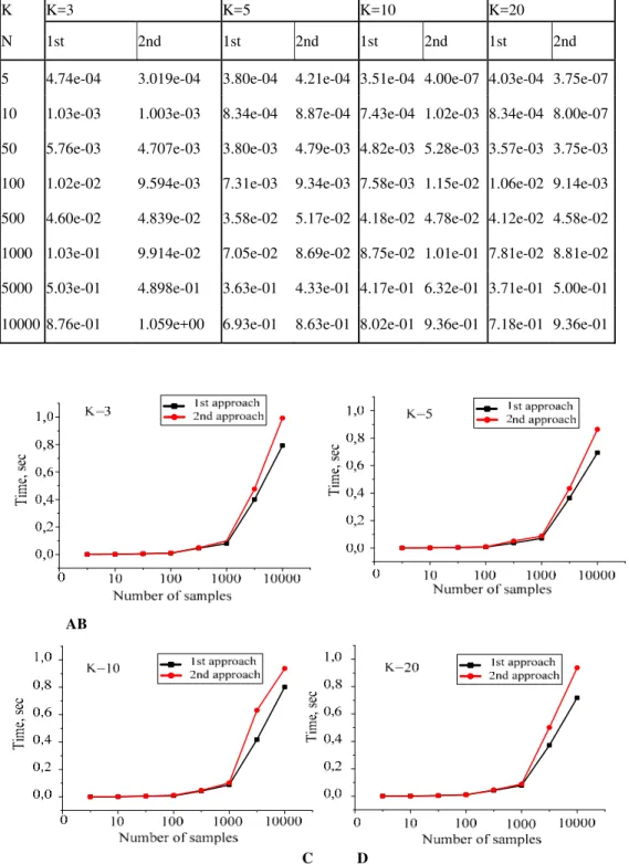
Table 1: Results of performance for two mixture generation approaches

K K=3 K=5 K=10 K=20

N 1st 2nd 1st 2nd 1st 2nd 1st 2nd

5 4.74e-04 3.019e-04 3.80e-04 4.21e-04 3.51e-04 4.00e-07 4.03e-04 3.75e-07

10 1.03e-03 1.003e-03 8.34e-04 8.87e-04 7.43e-04 1.02e-03 8.34e-04 8.00e-07

50 5.76e-03 4.707e-03 3.80e-03 4.79e-03 4.82e-03 5.28e-03 3.57e-03 3.75e-03

100 1.02e-02 9.594e-03 7.31e-03 9.34e-03 7.58e-03 1.15e-02 1.06e-02 9.14e-03

500 4.60e-02 4.839e-02 3.58e-02 5.17e-02 4.18e-02 4.78e-02 4.12e-02 4.58e-02

1000 1.03e-01 9.914e-02 7.05e-02 8.69e-02 8.75e-02 1.01e-01 7.81e-02 8.81e-02

5000 5.03e-01 4.898e-01 3.63e-01 4.33e-01 4.17e-01 6.32e-01 3.71e-01 5.00e-01

10000 8.76e-01 1.059e+00 6.93e-01 8.63e-01 8.02e-01 9.36e-01 7.18e-01 9.36e-01

AB

C D

Fig.5. Time of performance depending of sample size n and number of mixture components k

Figure 5illustrates that the first method of generation is little faster. As mentioned, according to this method we chose the component density for every point from the sample. Since the goal is to generate the data with fixed weighting probabilities, the second approach is easier to understandbecause the coefficient pi is simply

defined asNi/N, where Ni is the number of samples generated from th

4. Conclusion

This paper illustrated the computational features of mixture distributions through the analysis and simulation of two methods of data generation with Gaussian mixture PDF distributions. Using these two experimental approaches,a simulation of a Gaussian mixture was conducted, the M-PDF and weighted probabilities to simulate data from the mixture models were computed. We compared the two approaches and reported the results for the two mixture generation models. We reported the time of performance depending of sample size and number of mixture components. We found that the first method of generation was faster and the second method was easier to understand. In conclusions, either method is a reasonable approach to generation data with a Gaussian mixture PDF.

REFERENCES

1. Bowman, K.O. and Shenton, L.R. (2007). Mixture distributions and a test statistic. Far East Journal of Theoretical Statistics, 23(2), 241-259.

2. DeCarlo, L. (2002). Signal detection theory with finite mixture distributions: theoretical developments with applications to recognition memory. Psychological Review, 109(4), 710-721.

3. Dempster, A., Laird, N. and Rubin, D. (1977). Maximum likelihood for incomplete data via the EM algorithm. Jornal of the Royal Statistical Society, Series B (Methodological), 39(1), 1-38.

4. James, B.M. and Richard J.B. (1987). Some generalized mixture distributions with an application to unemployment duration. The

Review of Economics and Statistics, 69(2),232-240.

5. Leisch, R. F. (2003). FlexMix: A general framework for finite mixture models and latent class regression. Journal of Statistical Software.

6. McLachlan, G. and Krishnan, T. (1996). The EM algorithm and extensions. New York: John Wiley & Sons. 7. McLachan, G. and Peel, D. (2000). Finite mixture models. New York: JohnWiley & Sons.

8. Navidi, W. (1996). A graphical illustration of EM algorithm. The American Statistician, 51(1), 29-31.

9. Sattayatham, P. and Talangtam, P.(2012).Fitting of finite mixture distributions to motor insurance claims.Journal of Mathematics and Statistics, 8(1), 49-56.