Journal of Applied Fluid Mechanics, Vol. 10, No. 2, pp. 693-702, 2017. Available online at www.jafmonline.net, ISSN 1735-3572, EISSN 1735-3645. DOI: 10.18869/acadpub.jafm.73.238.27034
Three-Dimensional Numerical Simulation of Deformation
of a Single Drop under Uniform Electric Field
M. Akbari and S. Mortazavi
†Department of Mechanical Engineering, Isfahan University of Technology, Isfahan,8415683111, Iran
†Corresponding Author Email: [email protected] (Received August 6, 2016; accepted November 19, 2016)
A
BSTRACT
In this paper, deformation of a drop suspended in another immiscible fluid that is influenced by an external uniform electric field is investigated through fully 3D numerical simulations. The electric field is applied by imposing an electric potential difference in the ambient fluid. The Leaky dielectric model is used to obtain the electric field, charge distribution and eventually applied electric force at the interface. This force creates both oblate and prolate shapes, and also induces various Electrohydrodynamic flows inside and outside of the drop depending on the conductivity and permittivity ratio of the drop and the ambient fluid. A finite difference/front-tracking method is used. The results are presented for a wide range of non-dimensional parameters for predicting the drop deformation quantitatively and qualitatively. Different flow patterns are induced inside and outside of the drop. The results show a good agreement with theoretical and experimental results in the literature. For the sake of consideration of the problem in more detail, four specific cases are investigated.
Keywords: Oblate/prolate shape; Electric conductivity/permittivity; Front-tracking method.
N
OMENCLATUREa drop radius D drop deformation E∞ electric field Fel electric force
H the height of the domain L the length of the domain q electric charge
r density ratio
te charge relaxation time
th characteristic hydrodynamic time
W the width of the domain
γ interfacial tension
ε electric permittivity
εr electric permittivity ratio
ε0 electric permittivity of free space
viscosity ratio viscosity
ρ density
electric conductivity
r electric conductivity ratio
dimensionless time
ϕ electric potential Ф discrimination function
ω vorticity
1. I
NTRODUCTIONElectrohydrodynamics (EHD) as an interdisciplinary phenomenon, has recently been investigated by several researchers. In fact, EHD deals with both hydrodynamic flows influenced by electric currents and electric problems correlated with hydrodynamics. It has numerous applications like biotechnological processes, fuel atomization, ink jet printing, pumping, boiling, increasing heat and mass transfer and formation, transmission, coalescence and breakup of drops in microfluidic devices (Cho et al. 2003). A new application of this
1953 and Taylor 1964), Allan et al. (1962) experiments showed that both prolate and oblate shapes will occur. Taylor explained this phenomenon. He stated that, even a small conductivity in the ambient fluid can cause migration of free charges to the interface and eventually creating tangential stresses and inducing electrohydrodynamic flows inside and outside of the drop. The induced flow depends on the electric conductivity and permittivity of the drop and the ambient fluid. He proposed a linear theory which is well-known as leaky dielectric model and suggested a mathematic formulation for predicting the deformation of the drop qualitatively and quantitatively. Several investigators have used this model to solve the problem numerically. Sherwood did the first numerical simulation of the problem of a single drop in an electric field using boundary integral method in the limit of Stokes flow and found a good agreement with Taylor theory (Sherwood 1988). Tsukada et al. (1993) studied induced circulatory flows inside and outside of a drop using Galerkin finite element and found a good agreement with Taylor theory. Feng et al. (1996) simulated a single drop deformation in both Stokes and finite Reynolds numbers by using Galerkin finite element method. They found a good agreement with Taylor theory for small deformations although there was some discrepancy for large deformations. Also Feng investigated the effects of charge convection in leaky dielectric model for finite electric Reynolds numbers (Feng 1999). Zhang et al. (2005), studied numerical simulation of drop deformation using two dimensional Lattice-Boltzmann method for the first time and reported relevant results. Tomar et al. (2007) simulated drop deformation for perfect dielectrics and perfect conductors using VOF (volume of fluid) method and reported a good agreement with Taylor theory for small deformations. Lac et al. (2007) studied the effects of electric fields on a suspended drop in leaky dielectric model using axisymmetric boundary integral method. They also simulated the EHD breakup of drops. Hua et al. (2008) considered numerical simulation of drop deformation/motion with axisymmetric front-tracking method and using three perfect dielectric/conductor and leaky dielectric models. They found good agreement with Taylor theory. Herrera et al. (2011) used a charge convective approach for simulation of EHD problems using VOF method. They studied drop deformation and validated their results with Taylor theory. Paknemat et al. (2012) investigated the drop deformation and breakup for both perfect and leaky dielectric models using level set method. Yang et al. (2013) studied axisymmetric drop deformation through a 3D phase field model and reported that the drop takes different shapes until reaching steady state. Hu et al. (2015) developed a hybrid immersed boundary (IB) and immersed interface method (IIM) to simulate the dynamics of a drop in an electric field. They reported a good agreement with Taylor theory for small deformations. Simulation of several drops in a simple shear flow under uniform electric field was performed by Fernández (2008) in three dimensions. They studied the behaviour of
emulsion for leaky dielectric drops. However, they did not address the deformation of a drop under uniform electric field.
In this study, three dimensional numerical simulation of drop deformation suspended in another immiscible fluid under influence of external uniform electric field is investigated. The effects of hydrodynamics are absent and only the electrostatic forces cause the drop to deform in an oblate or prolate shape. Effect of hydrodynamics on the drop evolution is left for future investigations. Schematic configuration of domain along with non-dimensional parameters and governing equations is presented later, then the results are discussed and a conclusion will terminate this paper.
2. P
ROBLEMD
EFINITION ANDG
OVERNINGE
QUATIONS2.1
Flow Geometry
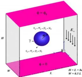
In this paper, the effect of external uniform electric field on a drop suspended in another immiscible liquid is investigated through fully 3D numerical simulations. A schematic of the problem is shown in Fig. 1. As shown in Fig. 1, the domain is a box that its length (L) is equal to its height (H). To remove the effects of the walls on drop behaviour, the drop radius is taken as one-eighth of the channel height. If the domain height increases, it does not change the results significantly. This has been checked but not included in the paper. The width (W) of the domain is one half of its length.
Fig. 1. Schematic of three dimensional domain for a drop suspended in another immiscible fluid
under the influence of an external uniform electric field.
The drop is initially spherical and stable at the centre of the domain. The electric field (E∞) is formed by applying a potential difference (
0)
wall-bounded in Z-direction and periodic in X and Y directions.
2.2
Non-Dimensional Parameters
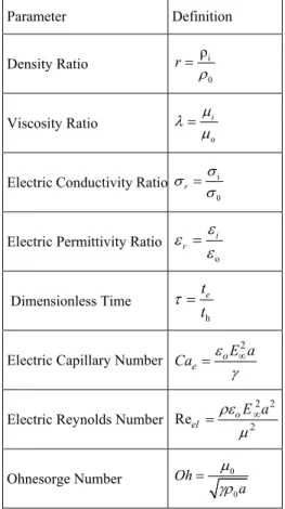
The most important dimensionless parameters in Electrogydrodynamics are listed in Table 1. Like Fig. 1, the subscripts i and o refer to the drop and the ambient fluid respectively.
Table 1 Non-dimensional parameters using in Electrohydrodynamics
Parameter Definition
Density Ratio i
0 ρ r Viscosity Ratio o i
Electric Conductivity Ratio i
0 r
Electric Permittivity Ratio o i r
Dimensionless Time h e t t
Electric Capillary Number
2 o e E a Ca
Electric Reynolds Number
2 2
2
Reel o
E a
Ohnesorge Number 0
0 Oh a
In all the simulations presented here, r 1. In definition of dimensionless time ( ), 0
e
t
is
charge relaxation time and
3
h
a
t is a characteristic hydrodynamic time. The electric permittivity of free space is 08.885 [pF/ m]. The leaky dielectric model is valid when is small. Because there is a relation between Oh and Reel
(
Re
e el
Ca
Oh ), one of them is set in EHD problems in addition to Cae.
2.3
Governing Equations
In microgravity multiphase flows, the buoyancy force is weak and surface tension is dominant. Therefore, other volume forces like electrostatic forces can cause fluid flow and deformation of the interface. The governing physics of EHD multiphase flows has been reviewed by several
authors including Melcher et al. (1969) and Saville (1997) who discussed leaky dielectric model for fluids with low conductivity. In leaky dielectric model the time scale associated with the relaxation of electric charges is small compared to time scale associated with the hydrodynamics of the flow. Thus the electrostatic field can be assumed to be quasi-steady, and a steady state equation for the conservation of charge can be considered:
. 0
(1) The electric field (E) is found by using electric potential (
)
through Eq. (2):E (2) One of the important features of EHD is irrotational electric field and electric dynamic currents are so weak that Faraday’s law of Induction is negligible. Therefore, there is no effect of magnetic field. Free charges (q) are found by using Gauss’ law as below:
.
qE (3) According to Melcher et al. (1969), electric force at the interface is due to jump of electric stresses. This volume force is as follows:
1 1
( . ) ( ( . ) )
2 2
El
F qE E E E E
(4) This force will act only at the interface if ε (electric permittivity) and (electric conductivity) are constant in each phase. In this equation, the first term is due to presence of free charges and in fact is proportional to density of free charges. The second term is the effect of difference in electric permittivity ratio of both fluids and is known as polarization force density. The last term which is usually ignored is due to variation in material density. In the current work, this term is neglected because the density of both phases are the same. The flow field is obtained through Navier-Stokes equations: . . ( ) ( ) T El u
u u P u u
t
n x x dA F
(5)Here u is velocity, P is pressure, ρ, and γ are density, viscosity and surface tension respectively, is the curvature and n is a unit normal to the interface.
(
x
x
)
, is a delta function that is zero everywhere except at the interface. The gravity is ignored in this problem. The continuity equation with assumption of incompressible fluids is:.u 0
both the convective and viscous terms. The equations are integrated in time by a second order predictor-corrector scheme. Combining the continuity and momentum equations leads to a pressure equation that is solved by a multigrid method. The equation for conservation of charge (Eq. (1)) is also discretized with standard central differences and is solved by the same multigrid scheme. The electric potential is stored at pressure nodes. The electrostatic forces are stored at the boundary of the cells, the location where the velocities are stored. The electrostatic forces are directly added in the predictor step in the projection method. In general, solving the Navier-Stokes equations is not an easy task when an interface exists at the phase boundary. The front-tracking method is capable of handling these types of flows due to its accuracy and its ability to consider the discontinuity across the interface. For a detailed discussion about the numerical method, the reader is referred to the work by Tryggvason et al. (2001).
2.4
Deformation and Induced Flows
As it was mentioned earlier, due to applying electric field, the drop will deform into both oblate and prolate shapes depending on the electrical properties of the fluid. Taylor suggested a linear theory known as Taylor theory to predict the EHD drop deformation (D) as follows (Taylor 1964):
2 2
9 3 2 3
1 2
16 2 5 1
e
r r r r
r Ca
D
(7)
Also the drop deformation is obtained from: L B
D L B
(8) Where L is the drop length parallel to electric field and B is the drop length perpendicular to electric field. In both equations, positive deformation (D > 0) shows prolate and negative deformation (D < 0) shows oblate shape.
Fig. 2. Deformation types regarding the sign of D and direction of the electric field.
Next, the induced flow types are considered. For this purpose, a discrimination function that is proposed by Taylor (1966) to determine the type of deformation and induced flows, is introduced. This function is defined for spherical drops as:
2 3 2 3
( 1) 2 1
5 1
r
r r
r
(9)
where Φ > 0 represents prolate shape and Φ < 0 shows oblate shape. According to Rhodes et al. (1989) solution, for two-dimensional drops and
1
, the discrimination function becomes:
2 2
Φd 1 3r r r (10) Figure 3 illustrates Eq. (10) in terms of electric conductivity versus electric permittivity. The bold line represents 2d 0. For locations below this
line ( 2d 0) the drop will deform into oblate
shape and above the line ( 2d 0) the drop has
prolate shape. The dashed line (rr) determines
the type of the induced flows. Below this (r r)
the flow is from the pole to the equator and above it (rr) the flow is from the equator to the poles.
Fig. 3. Map of drop behavior as a function of conductivity ratio and permittivity ratio based
on the leaky dielectric model. Solid line is discrimination function (Eq. (10)) and symbols
are case studies of present work.
3. R
ESULTSA
NDD
ISCUSSION3.1
Validation
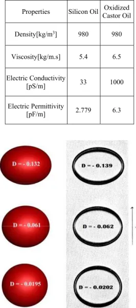
To examine the validity of the method (front- tracking coupled with electrostatic effects), the deformation obtained by Torza et al. (1971) using experiments (system 16, class C) are compared with the current work. In these cases, the drop and the ambient fluids are silicon and oxidized castor oils respectively. Three capillary numbers are considered (0.137, 0.380 and 0.745). The mechanical and electrical properties of these fluids are listed in Table 2.
Table 2 Mechanical and electrical properties of silicon and castor oils used in Torza et al. (1971)
experiments (sys 16-class C)
Properties Silicon Oil Oxidized Castor Oil
Density[kg/m3] 980 980
Viscosity[kg/m.s] 5.4 6.5
Electric Conductivity
[pS/m] 33 1000
Electric Permittivity
[pF/m] 2.779 6.3
Fig. 4. Comparison of the numerical simulation in the present work (left) and the experimental
results of Torza et al. (1971) (right).
3.2
Drop Deformation
Deformation of a single drop suspended in another immiscible fluid under uniform electric field (Fig. 1) is investigated in details. According to Eq. 7, the drop deformation is related to electric capillary number (Cae), viscosity ratio ( ), electric
conductivity and electric permittivity ratio ( r and εr).
The effect of these parameters on the drop deformation (except that is unity throughout the paper) is studied in a relatively wide range.
3.2.1
Grid Study
First, a grid resolution test is performed. Four grid resolutions are examined (64*32*64, 96*48*96, 128*64*128, 160*80*160). The flow conditions are: Cae 0.5, r2.0, r2.5 and the domain is the same as that is presented in Fig. 1. Fig. 5
shows the deformation versus time for four grid resolutions. It is clear that the grid resolution 96*48*96 is reasonably accurate, and the computational time to get steady state condition is also reasonable. This grid resolution is chosen for the rest of computations.
Fig. 5. Drop deformation versus time at different grid resolutions (Cae = 0.5, σr = 2.5 and εr = 2.0).
3.2.2
Effect of Electric Capillary Number
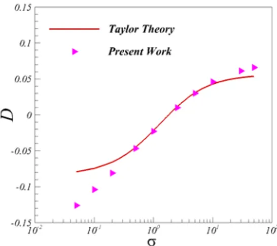
The effect of electric capillary number on drop deformation is presented in Fig. 6. This figure represents the drop deformation for various capillary numbers.
Fig. 6. Effect of electric capillary number on drop deformation and comparison with Taylor
theory (σr = 2.5 and εr = 2.0).
3.2.3
Effect of Electric Conductivity Ratio
The effect of electric conductivity ratio on drop deformation is depicted in Fig. 7. The drop deformation is plotted versus the conductivity ratio and compared with Taylor theory. Here the electric capillary number is Cae0.1and permittivity ratio is r 2.0. The drop deformation increases with conductivity ratio. This can be due to migration of more charges to the interface as the conductivity increases. This trend has also been reported by Hua et al. (2008), Herrera et al. (2011) and Yang et al. (2013). Here deviation from Taylor theory for large deformations (D 0.05) is also visible.
Fig. 7. Effect of electric conductivity ratio on drop deformation and comparison with Taylor
theory (Cae = 0.1 and εr = 2.0).
3.2.4
Effect of Electric Permittivity Ratio
The effect of electric permittivity ratio on drop deformation is illustrated in Fig. 8. It is also compared with Taylor theory. It can be seen that at low permittivity ratios the drop has a prolate shape. However, it changes to oblate shape at large permittivity ratios. The results are nearly compatible with Taylor theory. Again discrepancy between Taylor theory and simulations at large deformations (D 0.05) is visible. As it was mentioned earlier this matter is due to the fact that linear theory is valid for small deformation. The Ohnesorge number is taken as Oh0.289 in simulations presented in Figs. 6, 7 and 8.
The results presented in Fig. 6 through 8, cannot be compared to results by Hua et al. (2008) (an axisymmetric simulation) although they had similar trends. There is a mistake in the formula that they used to calculate drop deformation (a factor of 1/2 is missing). Also the same mistake is repeated when calculating the drop deformation from numerical simulations.
3.3
Induced Flows
As it mentioned earlier, in leaky dielectric model, there are two different flow patterns for a drop suspended in another immiscible fluid under
influence of external uniform electric field. One is from the poles to the equator and the other is from the equator to the poles. This depends on electric conductivity and permittivity ratios of the drop and the ambient fluid. To examine these flow patterns, four simulations in different regions of the Fig. 3 are performed. These points are shown in the Fig. 3 with numbers 1, 2, 3 and 4. In these simulations, the electric Reynolds number in addition to electric capillary number are used as dimensionless parameters to characterise the problem. Electric Reynolds number is set to Reel 0.1 for all simulations and electric capillary number is set to
0.25
e
Ca for cases 1, 2 and 3 and Cae 1.0 for case 4. For case 1, r 5 and r0.5. Therefore,
Ф2d (Eq. (10)) becomes negative ( 2d 13.25)
and as a result, the drop becomes oblate.
Fig. 8 Effect of electric permittivity ratio on drop deformation and comparison with Taylor theory
(Cae = 0.1 and σr = 2.5).
Fig. 9. Electric potential contours (left) and streamlines (right) inside and outside of the drop
for case 1. (Cae = 0.25, σr = 2.5 and εr = 5.0).
Also because the electric conductivity ratio is lower than electric permittivity ratio (r r), the flow
pattern is from the pole to the equator. Fig. 9 represents electric potential distribution (left) in the whole domain in addition to streamlines (right) inside and outside of the drop. The streamlines around the drop at steady state are presented in Fig. 10.
the present numerical method. For case 2, r 15 and r 10. Furthermore, Ф2d is positive in Eq. (10) ( 2d 66) and the drop has a prolate shape.
Fig. 11 illustrates both electric potential distribution (left) and streamlines (right) inside and outside of the drop.
Fig. 10. 3-D deformed drop and outside streamlines for case 1. (Cae = 0.25, σr = 2.5
and εr = 5.0).
Fig. 11. Electric potential contours (left) and streamlines (right) inside and outside of the drop
for case 2. (Cae = 0.25, σr = 10 and εr = 15).
Also Fig. 12 depicts 3D deformed drop and streamlines around it for case 2. It is clear that the flow patterns inside and outside of the drop for this case is similar to case 1 because the electric conductivity ratio is lower than electric permittivity ratio (rr), for both cases. Again the
streamlines are presented in a plane at the middle of the domain (Y W 2). Case 3 in Fig. 3 has
0.5
r
and r20. Accordingly, Ф2d is 420, and the drop has a prolate shape.
But in contrast to cases 1 and 2, for this case the electric conductivity ratio is higher than electric permittivity ratio (rr). As a result, the flow
pattern is in contrast to the case 1 and 2 (the flow is from equator to poles).
Figure 13 shows the electric potential distribution (left) and streamlines inside and outside of the drop (right).
Fig. 12. 3-D deformed drop and outside streamlines for case 2. (Cae = 0.25, σr = 10
and εr = 15).
Fig. 13. Electric potential contours (left) and streamlines (right) inside and outside of the drop
for case 3. (Cae = 0.25, σr = 20 and εr = 0.5).
Fig. 14. 3-D deformed drop and outside streamlines for case 3. (Cae = 0.25, σr = 20
and εr = 0.5).
Figure 14 illustrates the 3D deformed drop with streamlines around it. Streamlines in Fig. 13 and 14 are obtained in a plane at the middle of the domain (Y W 2). It is clear from these Figures, that the streamlines are as expected as flow patterns according to the Fig. 3.
parameters are also set as: r 0.05and r 0.01.
Here Ф2d becomes positive (0.086). Therefore, the
drop becomes prolate. But because the electric conductivity ratio is lower than electric permittivity ratio, the flow patterns are similar to cases 1 and 2. Fig. 15 illustrates the electric potential distribution (left) and streamlines inside and outside of the drop (right).
Fig. 15. Electric potential contours (left) and streamlines (right) inside and outside of the drop
for case 4. (Cae = 1.0, σr = 0.01 and εr = 0.05).
It should be noted that, generally the curved distribution of electric potential lines around the drop is due to electric conductivity difference between the drop and the ambient fluid. This is visible in Figs. 9, 11, 13 and 15. However, the curvature of electric potential lines for case 4 is different because in this case the conductivity of the ambient fluid is higher than the conductivity of the drop. Fig. 16 represents the streamlines for case 4 around the 3D deformed drop.
Fig. 16. 3-D deformed drop and outside streamlines for case 4. (Cae = 1.0, σr = 0.01
and εr = 0.05).
To quantify the strength of the induced flows in these cases (cases 1 through 4 in Fig. 3), magnitude of vorticity vector (|ω|, enstrophy) for each case in addition to absolute drop deformation (|D|) are presented in Table 3.
It is obvious that for cases 2 and 4 (prolate drops with streamlines similar to oblate drops) both drop deformation and vorticity are less than case 1 and 3. Thus, one can concludes that for prolate drops with
r r
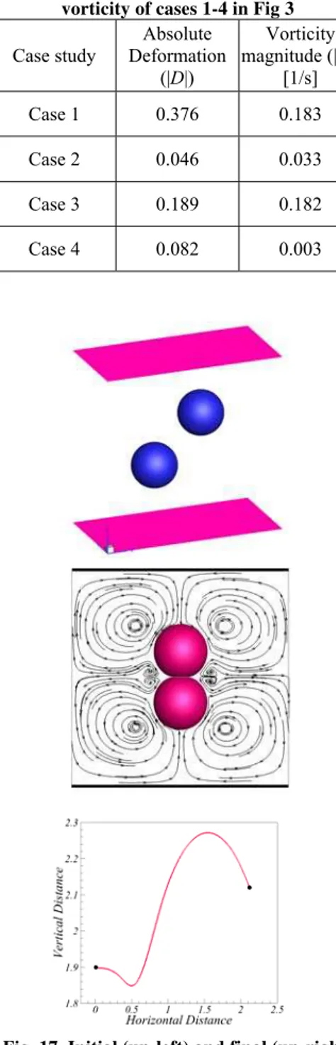
(cases 2 and 4), drop deformation is smaller in comparison to other prolate and oblate drops (cases 1 and 3). This is due to weaker induced flows caused by the electric field for drops 2 and 4. To show superiority of fully three dimensional simulations presented in this study against axisymmetric case, the interaction of two drops is also simulated. The drops are initially located in a line with an angle of 45 degrees with respect to Z-direction. Fig. 17, depicts initial (up-left) and final (up-right) configuration of drops in addition to streamlines around them.
Table 3 Absolute values of deformation and vorticity of cases 1-4 in Fig 3
Case study
Absolute Deformation
(|D|)
Vorticity magnitude (|ω|)
[1/s] Case 1 0.376 0.183 Case 2 0.046 0.033 Case 3 0.189 0.182 Case 4 0.082 0.003
The evolution of drops with respect to each other are also presented in Fig 17 by comparing their horizontal and vertical distance. The domain and drops size are exactly similar to Fig. 1. Here, non-dimensional parameters are: Cae 0.1, 0.2Oh ,
8
r
and r 6.
4. C
ONCLUSIONIn this paper, coupling of electrostatic effects with hydrodynamics was done in three dimensions to investigate drop deformation in an electric field. The deformation of a single drop suspended in another immiscible fluid under influence of external uniform electric field is studied through numerical simulations. The electric force, was added to the flow equations to investigate its effects on the drop deformation and the induced flows. A front-tracking/finite difference method was used and was validated based on the existing experimental and theoretical results. The method efficiently predicts both the drop deformation and the induced electrohydrodynamic flows inside and outside of the drop. It should be pointed out that, in this paper the effects of hydrodynamics are absent and is left for future work. Therefore, only electrostatic forces are presented and the drop deforms due to these forces. Since the real physics is captured in three dimensional simulations, the method can be applied to various problems to show their real behaviour.
R
EFERENCESAllan, R. and S. Mason (1962). Particle behaviour in shear and electric fields. I. Deformation and burst of fluid drops. In Proceedings of the Royal Society of London. Series A. Mathematical and Physical Sciences 267(1328), 45-61.
Basaran, O. A. and L. Scriven (1990). Axisymmetric shapes and stability of pendant and sessile drops in an electric field. Journal of Colloid and Interface Science 140(1), 10-30. Cho, S. K., H. Moon and C. J. Kim (2003).
Creating, transporting, cutting, and merging liquid droplets by electrowetting-based actuation for digital microfluidic circuits. Journal of Microelectromechanical Systems 12,70-80.
Feng, J. Q. (1999). Electrohydrodynamic behaviour of a drop subjected to a steady uniform electric field at finite electric Reynolds number. Proceedings of the Royal Society of London A: Mathematical, Physical and Engineering Sciences 455(1986), 2245-2269.
Feng, J. Q. and T. C. Scott (1996). A computational analysis of electrohydrodynamics of a leaky dielectric drop in an electric field. Journal of Fluid Mechanics 311, 289-326.
Fernández, A. (2008). Response of an emulsion of leaky dielectric drops immersed in a simple shear flow: Drops less conductive than the
suspending fluid. Phys. Fluids 20(4).
Hua, J., L. K. Lim and C. H. Wang (2008). Numerical simulation of deformation/motion of a drop suspended in viscous liquids under influence of steady electric fields. Physics of Fluids (1994-present) 20(11).
Hu, W. F., M. C. Lai and Y. N. Young (2015). A hybrid immersed boundary and immersed interface method for electrohydrodynamic simulations. Journal of Computational Physics 282, 47-61.
Lac, E. and G. Homsy (2007). Axisymmetric deformation and stability of a viscous drop in a steady electric field. Journal of Fluid Mechanics 590, 239-264.
López-Herrera, J., S. Popinet and M. Herrada (2011). A charge-conservative approach for simulating electrohydrodynamic two-phase flows using volume-of-fluid. Journal of Computational Physics 230(5), 1939-1955. Melcher, J., and G. Taylor (1969).
Electrohydrodynamics: A review of the role of interfacial shear stresses. Annual Review of Fluid Mechanics 1(1), 111-146.
O'Konski, C. T. and H. C. Thacher Jr (1953). The distortion of aerosol droplets by an electric field. The Journal of Physical Chemistry 57(9), 955-958.
Paknemat, H., A. Pishevar and P. Pournaderi (2012). Numerical simulation of drop deformations and breakup modes caused by direct current electric fields. Physics of Fluids (1994-present) 24(10), 102101.
Rhodes, P. H., R. S. Snyder and G. O. Roberts (1989). Electrohydrodynamic distortion of sample streams in continuous flow electrophoresis. Journal of Colloid and interface Science 129(1), 78-90.
Saville, D. (1997). Electrohydrodynamics: The Taylor-Melcher leaky dielectric model. Annual Review of Fluid Mechanics 29(1), 27-64. Sherwood, J. (1988). Breakup of fluid droplets in
electric and magnetic fields. Journal of Fluid Mechanics 188, 133-146.
Taylor, G. (1964). Disintegration of water drops in an electric field. In Proceedings of the Royal Society of London. Series A. Mathematical and Physical Sciences 280(1382), 383-397. Taylor, G. (1966). Studies in electrohydrodynamics.
I. The circulation produced in a drop by electrical field. In Proceedings of the Royal Society of London. Series A. Mathematical and Physical Sciences 291(1425), 159-166. Tomar, G., D. Gerlach, G. Biswas, N. Alleborn, A.
Torza, S., R. Cox and S. Mason (1971). Electrohydrodynamic deformation and burst of liquid drops. Philosophical Transactions of the Royal Society of London. Series A, Mathematical and Physical Sciences 269(1198), 295-319.
Tryggvason, G., B. Bunner, A. Esmaeeli, D. Juric, N. Al-Rawahi, W. Tauber, and Y. J. Jan (2001). A front-tracking method for the computations of multiphase flow. Journal of Computational Physics, 169(2), 708-759. Tsukada, T., T. Katayama, Y. Ito and M. Hozawa
(1993). Theoretical and experimental studies of circulations inside and outside a deformed drop under a uniform electric field. Journal of Chemical Engineering of Japan 26(6), 698-703.
Unverdi, S. O. and G. Tryggvason (1992). A front-tracking method for viscous, incompressible, multi-fluid flows. Journal of Computational Physics 100(1), 25-37.
Yang, Q., B. Q. Li, and Y. Ding (2013). 3D phase field modeling of electrohydrodynamic multiphase flows. International Journal of Multiphase Flow 57, 1-9.
Zeng, J. and T. Korsmeyer (2004). Principles of droplet electrohydrodynamics for lab-on-a-chip. Lab on a Chip 4, 265-277.