www.earth-syst-sci-data.net/8/461/2016/ doi:10.5194/essd-8-461-2016
© Author(s) 2016. CC Attribution 3.0 License.
The Stratospheric Water and Ozone Satellite
Homogenized (SWOOSH) database: a long-term
database for climate studies
Sean M. Davis1,2, Karen H. Rosenlof1, Birgit Hassler1,2, Dale F. Hurst1,2, William G. Read3, Holger Vömel4, Henry Selkirk5,6, Masatomo Fujiwara7, and Robert Damadeo8
1NOAA Earth Systems Research Laboratory (ESRL), Boulder, CO, USA
2Cooperative Institute for Research in Environmental Sciences (CIRES), University of Colorado at Boulder,
Boulder, CO, USA
3Jet Propulsion Laboratory, California Institute of Technology, Pasadena, CA, USA 4National Center for Atmospheric Research, Boulder, CO, USA
5NASA Goddard Space Flight Center, Greenbelt, MD, USA 6Universities Space Research Association, Columbia, MD, USA
7Hokkaido University, Sapporo, Japan 8NASA Langley Research Center, Hampton, VA, USA
Correspondence to:Sean M. Davis ([email protected]) Received: 4 May 2016 – Published in Earth Syst. Sci. Data Discuss.: 18 May 2016 Revised: 2 September 2016 – Accepted: 8 September 2016 – Published: 28 September 2016
Abstract. In this paper, we describe the construction of the Stratospheric Water and Ozone Satellite
Homoge-nized (SWOOSH) database, which includes vertically resolved ozone and water vapor data from a subset of the limb profiling satellite instruments operating since the 1980s. The primary SWOOSH products are zonal-mean monthly-mean time series of water vapor and ozone mixing ratio on pressure levels (12 levels per decade from 316 to 1 hPa). The SWOOSH pressure level products are provided on several independent zonal-mean grids (2.5, 5, and 10◦), and additional products include two coarse 3-D griddings (30◦long×10◦lat, 20◦×5◦) as well as
lower stratosphere (UTLS) region (Forster and Shine, 1999; Forster et al., 2007; Maycock et al., 2011; Solomon et al., 2010).
Despite their chemical and radiative importance in the stratosphere, there have been relatively few attempts at con-structing long-term data records of O3 and WV based on
vertically resolved satellite limb-based observations of these species. To aid in the study of variability and change in water vapor and ozone in the upper troposphere to strato-sphere region, we have constructed the Stratospheric Water Vapor and Ozone Satellite Homogenized (SWOOSH) data set. SWOOSH is a global long-term vertically resolved grid-ded database of satellite O3/WV measurements that has been
designed with the goal of accurately reproducing the monthly average variability present in the underlying data. SWOOSH can be used as input to global models to test sensitivity to changes in ozone or water vapor, as well as for comparison with model output. In this paper, we describe the construc-tion of the database, which includes new data filtering and homogenization algorithms.
Although several efforts have been made to combine the overlapping satellite ozone measurements into gridded, ver-tically resolved time series (e.g., Cionni et al., 2011; Ran-del and Wu, 2007; Bodeker et al., 2013; Froidevaux et al., 2015), to date there have been fewer attempts to create a ho-mogenized satellite record of vertically resolved water va-por (Hegglin et al., 2014; Froidevaux et al., 2015). This is no doubt partly due to gaps in the satellite data records as well as to well-documented disparities between satellite and in situ measurements of water vapor (e.g., Kley et al., 2000).
Satellite vertical profile measurements of ozone and WV date back to Stratospheric Aerosol and Gas Experiment (SAGE I, ozone only, 1979–1981) and Limb Infrared Mon-itor of the Stratosphere (LIMS, 1978–1979; Gille and Rus-sell, 1984; Remsberg et al., 1984), but unfortunately these records do not overlap with subsequent satellite data sets. Continuous coverage of ozone/WV vertical profiles from satellites begins only with the SAGE II instrument in Oc-tober 1984. Since then, several other NASA satellite O3/WV
sounders have been launched; these include the Upper Atmo-spheric Research Satellite Halogen Occultation Experiment (UARS HALOE, 1991–2005), the UARS Microwave Limb
Randall, 2003; Wang et al., 2002); around 1 hPa the diurnal cycle of ozone becomes prominent and local time sampling must be taken into account (Sakazaki et al., 2015). In con-trast, water vapor retrievals from the various satellite instru-ments can exhibit biases of 20 % or more relative to one an-other, depending on the level, geographic location, and com-bination of instruments (Kley et al., 2000; Hegglin et al., 2013). Thus, a key aspect of any long-term WV data merg-ing is the requirement for some homogenization procedure to account for measurement offsets. Previous efforts to com-bine WV measurements have either used a model as a trans-fer standard (Hegglin et al., 2014) or have averaged data from the source satellite records (Froidevaux et al., 2015). In SWOOSH, data homogenization is accomplished by cal-culating instrument offsets using satellite–satellite coincident measurements taken during overlap time periods and apply-ing these offsets to adjust the data to those of a “reference” satellite.
The rest of this paper is organized as follows: in Sect. 2, we present the satellite data sets used in this study and discuss the screening that has been applied to the data. In Sect. 3, we discuss the process of choosing a reference satellite in-strument to which other data are adjusted. In Sect. 4, we describe the data homogenization, gridding, and combining process, including uncertainty estimation. Finally, in Sect. 5, we present examples of the utility of the long-term record for capturing seasonal to interannual variability.
2 Data and basic screening
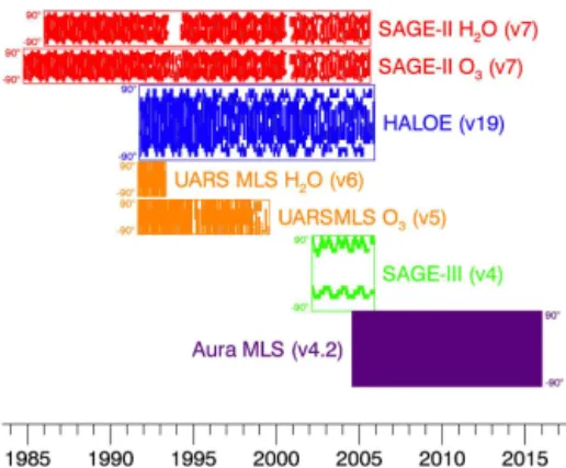
In this section, the SWOOSH satellite input data and screen-ing procedures are described. Currently, SWOOSH contains data from several satellite instruments: SAGE II, SAGE III, HALOE, UARS MLS, and EOS Aura MLS (hereafter Aura MLS). Basic information about these instruments including their operating periods and vertical resolutions is shown in Fig. 1 and Table 1. This subset of available satellite data was chosen because each instrument provides vertical profiles of both O3 and WV with roughly similar vertical resolution
Table 1.Overview of satellite data included in SWOOSH.
Instrument Data version
Start date
End date
H2O vertical resolution (km)
O3 vertical resolution (km)
H2O vertical range
O3 vertical range
SAGE II 7 (O3) 7 (H2O)
Oct 1984 Jan 1986
Aug 2005 Aug 2005
1a 1a 0.5–50 kmb 0.5–70 kmb
UARS HALOE 19 Oct 1991 Nov 2005 2 2.3 316–
0.002 hPa
584– 0.0004 hPa
UARS MLS 5 (O3) 6 (H2O)
Oct 1991 (H2O) Sep 1991 (O3)
Apr 1993 Nov 2005
3–4c 3.5–5d 100–
0.17 hPa
100– 0.22 hPa
SAGE III 4 Feb 2002 Nov 2005 1.5 1 0.5–
100 kmb 8–49 kme 384– 0.45 hPae
0.5– 100 kmb 1–82 kme 905– 0.007 hPae
Aura MLS 4.2 Aug 2004 present 2.5–3.5 2.5–3.5 316–
0.002 hPa
261– 0.02 hPa
aFWHM of triangular smoothing applied to balloon data for intercomparisons.bRetrieval grid.c3.5 km FWHM used for UARS MLS WV smoothing. d4 km FWHM used for UARS MLS O
3smoothing.eRange of valid values from raw data, before any screening.
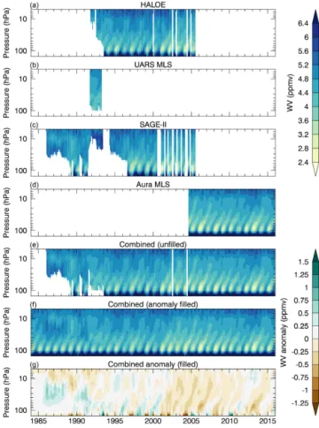
Figure 1.Temporal and latitudinal coverage of satellite data used as input to SWOOSH. The boxes surrounding each data set span 90◦S–90◦N in the vertical. Data are filled for each month and 10◦ latitude band containing valid data. Where significant coverage dif-ferences exist for WV and O3for a given satellite, the coverage is plotted separately.
several other satellite instruments that could be added dur-ing the 2000s, these data are not included because the Aura MLS provides sufficient sampling and global coverage on a monthly timescale.
Below, a brief description of each satellite instrument and the “basic” data screening is given. Basic screening is based on the published recommendations of the satellite instrument teams.
2.1 SAGE II and SAGE III
SAGE instruments provide water vapor, ozone, and aerosol profiles from measurements of solar radiation attenuated through the Earth’s limb during sunrise/sunset events viewed from the satellites’ orbits. SAGE II was launched in October 1984 aboard the Earth Radiation Budget Satellite (ERBS) and made measurements spanning 80◦S–80◦N until
Au-gust 2005. SAGE II was a seven-channel photometer mea-suring in the range from 0.385 to 1.02 µm (McCormick, 1987), with water vapor (ozone) retrieved from the channel at 0.935 µm (0.6 µm). SAGE III was launched into a Sun-synchronous orbit (100◦inclination) on 10 December 2001,
aboard the Russian Meteor 3M platform. In this orbit, so-lar occultation measurements were made at 47–84◦latitude
in the NH and 31–57◦ in the SH. SAGE III operated
un-til November 2005, measuring in 87 channels ranging from 0.290 to 1.54 µm.
SAGE II water vapor data are filtered according to the pub-lished recommendations of Taha et al. (2004) and Rind et al. (2005) to remove poor-quality retrievals and profiles im-pacted by high volcanic aerosol loading (e.g., following the eruption of Mt. Pinatubo in 1991). Specifically, we remove any points with water vapor uncertainty >50 %.
Addition-ally, we remove all data in a profile below the highest alti-tude point at which either cloud presence is flagged orβ1020
(1020 nm extinction)>2×10⁻⁴ km−1 and all profiles
as-sociated with “short events” during 1993–1994, as described in Taha et al. (2004).
Because the above screening fails to remove all data with clearly unphysical values, we apply additional outlier screen-ing. First, we remove extreme outliers, defined as H2O
mix-ing ratio>30 ppmv above 100 hPa. Then, we remove points
farther than 3σ from the mean at each level in 10◦latitude
bins. This results in the removal of an additional 0.6 % of the H2O data, with 80 % of the screened data being high outliers.
For SAGE II ozone, we filter data based on the recom-mendations of Wang et al. (2002, based on v6.1 data), with the additional criteria set forth in the SAGE II version 7.0 release notes. As with the SAGE II water vapor, this fil-tering removes aerosol contaminated and poor-quality re-trievals. The Wang et al. (2002) filtering involves discard-ing all points in a profile below which any of the crite-ria are met: β525 (525 nm extinction) >6×10⁻³km−1, or
1×10⁻³< β525<6×10⁻³km−1 andβ525/β1020<1.4, or
cloud presence flagged. Additionally, any profile that con-tains an uncertainty >10 % between 30 and 50 km is
en-tirely removed. Finally, individual points where uncertainty is greater than 300 % (at and above 35 km) or 200 % (below 35 km) are removed. In addition to the recommended screen-ing, the same 3σfiltering is applied to ozone as with the
wa-ter vapor data. This results in an additional removal of 0.6 % of the ozone data, with 70 % of the screened data being high outliers.
For SAGE III data, the data were prescreened by the re-trieval team, so with one exception no additional screening is necessary. The only screening applied to SAGE III data is removal of a few weeks worth of bad data during 2002, fol-lowing the recommendations of Thomason et al. (2010). We also apply a 3σ filtering, as with the SAGE II data. This
re-which switched every 36 days.
Water vapor profiles in the stratosphere and mesosphere were retrieved using the 183 GHz radiometer, which op-erated from September 1991 until April 1993. We use the UARS MLS version 6 data (Pumphrey, 1999; Pumphrey et al., 2000), which is retrieved at six levels per decade of pressure (resulting in ∼2.5 km vertical resolution) and produces useable profiles between about 100 and 0.1 hPa. The UARS MLS vertical resolution is approximately 3–4 km throughout most of the stratosphere (Pumphrey, 1999). Profiles containing negative uncertainty values are removed, which is equivalent to filtering out any of the bad MMAF_STAT quality flags related to unstable or unphysical retrievals (http://browse.ceda.ac.uk/browse/badc/mlsl3/ data/NERC-Edinburgh-h2o/v0006-edinburgh-h2o-official/ 00README_for_v0104).
Ozone was retrieved separately from both the 183 and 205 GHz channels, but we use only the 205 GHz version 5 ozone; it is the recommended product for stratospheric ozone, and it extends through the end of the UARS mis-sion, unlike the 183 GHz product (Livesey et al., 2003). Like the water vapor product, ozone is retrieved at six levels per decade of pressure. Ozone data are filtered based on the cri-teria of Livesey et al. (2003). In particular, only data with QUALITY_O3_205=4 are used, and data with negative un-certainty or bad MMAF_STAT quality flags are removed. Also, only ozone data between 100 and 1 hPa are used.
2.3 UARS HALOE
In addition to UARS MLS, the Halogen Occultation Experi-ment (HALOE) operated on board UARS from October 1991 until November 2005, making solar occultation measure-ments in the infrared (2.45–10.0 µm) with latitudinal cover-age from 80◦S to 80◦N (Russell III et al., 1993). HALOE
the HALOE version 19 (v19) products, which have been ex-tensively compared with independent satellite, balloon, and ground-based measurements (Kley et al., 2000; Hegglin et al., 2013; Nedoluha et al., 2007).
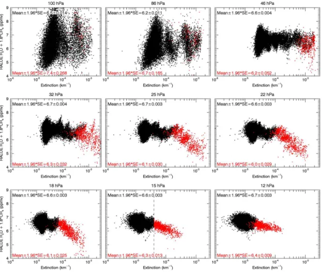
The HALOE ozone and water vapor data are filtered by first removing any “trip angle” or “constant lockdown angle” events identified by the data providers (http://haloe.gats-inc. com/user_docs/index.php). Then, any points with uncertain-ties≥100 % are removed (E. Remsberg, personal communi-cation, 2012). Finally, we apply an additional aerosol screen-ing procedure to remove affected profiles after the eruption of Mt. Pinatubo. Briefly, we remove any profiles where the NO-channel extinction at 15 hPa is greater than 4×10⁻⁵km−1.
The reasoning for this is illustrated in Fig. 2, which shows the plot of “total water” (H2O+1.8·CH4) vs. HALOE
NO-channel extinction for tropical data (30◦S–30◦N) at a
num-ber of different pressure levels. “Total water” is roughly con-stant in the tropical stratosphere (e.g., see Fig. 7 in Le Texier et al., 1988, and Table 1 in Dessler and Kim, 1999), and there are no physical reasons that it should depend on aerosol ex-tinction. Indeed, at lower extinction values there is no corre-lation between total water and extinction. However, at 15 hPa there is a clear dependence of total water on extinction for ex-tinction values above ∼4×10⁻⁵km. The mean total water
values at each pressure level are listed in Fig. 2 for profiles withβ15 hPa(NO-channel extinction at 15 hPa) greater than
or less than 4×10⁻⁵km−1. From these numbers, it is
appar-ent that profiles with high extinction at 15 hPa are dry bi-ased at the upper levels and wet bibi-ased at the lowest levels in the stratosphere. To remove these events, we discard the pro-file at altitudes below 15 hPa whenβ15 hPa>4×10⁻⁵km−1.
All profiles screened by this new algorithm occurred before November 1992 in the first year of operation of HALOE, when volcanic aerosols from the Mt. Pinatubo eruption heav-ily affected the profiles.
2.4 EOS Aura MLS
The Aura MLS instrument was launched in July 2004 aboard NASA’s EOS Aura satellite (Waters et al., 2006). The Aura MLS instrument measures thermally emitted microwave ra-diation from the Earth’s limb using five radiometer channels spanning 118 GHz to 2.5 THz; ozone is retrieved from the 240 GHz channel (Froidevaux et al., 2008; Jiang et al., 2007; Livesey et al., 2008), and water vapor is retrieved from the 190 GHz channel (Lambert et al., 2007; Read et al., 2007). The Aura MLS obtains∼3500 profiles per day and achieves nearly global coverage between 82◦S and 82◦N. Vertical
resolution generally increases as a function of height in the stratosphere for both retrievals but is 2.8–3.5 km for water and 2.5–3 km for ozone between 100 and 1 hPa. Over this same range, the estimated accuracy for ozone and water va-por is∼5–10 %. For both products, we use version 4.2 data, which are provided at 12 levels per decade (∼1.25 km) be-low 1 hPa.
The data filtering for the Aura MLS data is similar to that for version 2.2 data discussed in Lambert et al. (2007) for water vapor and Froidevaux et al. (2008) for ozone, but with updated values presented in the Aura MLS ver-sion 4.2 data quality document (http://mls.jpl.nasa.gov/data/ v4-2_data_quality_document.pdf).
Additional filtering that has been applied to the Aura MLS WV data to remove low-biased data in the UTLS is described in Appendix A. This filtering is motivated by the dry bias present in the MLS data, as described in the next section. This appendix describes a new algorithm for screening out Aura MLS WV profiles in the UTLS that are dry biased and contain unphysical oscillations. The motivation for Appendix A is that rather than simply remove all MLS data below a predetermined pressure level, it is desirable to retain as much of the Aura MLS data in the UTLS region (e.g., at lower latitudes) that are thought to be unaffected by the dry bias. The screening procedure described in Appendix A has been applied to all Aura MLS WV data stored in SWOOSH, so no action on the part of SWOOSH users is required.
3 In situ balloon measurements vs. satellite observations: choosing a reference satellite measurement
In this section, we compare balloon-borne ozone and frost point (FP) hygrometer sounding measurements to coincident satellite observations. These comparisons are used to quan-tify biases of the various satellite measurements, to idenquan-tify additional filtering that is needed for the satellite data, and to justify our choice of Aura MLS for water vapor and SAGE II for ozone as the reference measurements to which other mea-surements are adjusted.
3.1 Frost point hygrometer comparisons
Figure 2. HALOE “total water” (H2O+1.8·CH4) vs. aerosol extinction in the HALOE NO channel for tropical (30◦S–30◦N) data, segregated by events with low extinction (<4×10⁻⁵km−1, black) and high extinction (>4×10⁻⁵km−1, red) at 15 hPa. The mean ±1.96·standard error of the mean (i.e., the 95 % confidence interval) is given for each level and extinction category.
and the research vesselMiraicampaign in the tropical Indian Ocean (Suzuki et al., 2013).
Matched satellite profiles are found by searching for any profiles within a given time, distance, and equivalent latitude range of the FP data. Potential vorticity (PV)-based equiva-lent latitude from the MERRA reanalysis (Rienecker et al., 2011) is used as a match criterion because it allows for sim-ilar air masses to be identified (e.g., Manney et al., 2007). For all data except Aura MLS, the match criteria used are ±2 days, ±2000 km E–W distance (±18◦ longitude at the Equator), and±1000 km N–S distance (±9◦latitude). Due to the significantly better horizontal coverage for Aura MLS, the match criteria are stricter:±0.75 days,±1000 km E–W, and±500 km N–S, as used in Hurst et al. (2014). Addition-ally, for all data sets, we require the average equivalent lat-itude (between 316 and 68 hPa) to be within 5◦of the
cor-responding average equivalent latitude from the FP. If more than one profile meets the above criteria, the profile with the
closest equivalent latitude to the FP measurement is chosen. Using these match criteria, 1150 of the FP profiles are iden-tified as being matched with one or more satellite measure-ments.
For direct comparison with the satellite data, the FP data are averaged from their native resolution to that of the satel-lite using either the averaging/smoothing operators (for Aura MLS) or a triangular smoothing with full width at half max-imum (FWHM) equal to the instrument resolution (see Ta-ble 1), and then all data sets are interpolated onto the 12 lev-els per decade Aura MLS vertical grid for comparison pur-poses. Finally, for each level, any outlier pairs that are more than 5 standard deviations from the mean percent difference between the satellite and FP data are removed.
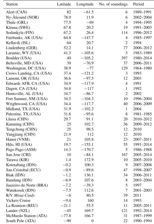
Table 2.Frost point hygrometer stations used in satellite water vapor intercomparison.
Station Latitude Longitude No. of soundings Period
Alert (CAN) 82 −61.5 6 1989–1991
Ny-Ålesund (NOR) 78.9 11.9 6 2002–2004
Thule (GRL) 77.5 −69 4 1994–1995
Kiruna (SWE) 67.8 20.2 19 1991–2003
Sodankyla (FIN) 67.2 26.4 114 1996–2012
Fairbanks, AK (USA) 64.8 −147.7 4 1985–1997
Keflavik (ISL) 64 20.7 2 1994
Lindenberg (GER) 52.2 14.1 77 2006–2012
Laramie, WY (USA) 41.3 −105.6 5 1983–1989
Boulder (USA) 40 −105.2 397 1980–2014
Beltsville, MD (USA) 39 −76.9 37 2006–2011
Washington, DC (USA) 38.9 −77 129 1964–1980
Crows Landing, CA (USA) 37.4 −121.2 3 1993
Lamont, OK (USA) 36.6 −97.5 12 2003
Edwards AFB, CA (USA) 34.9 −117.9 4 1991
Dagett, CA (USA) 34.8 −117 1 1992
Huntsville, AL (USA) 34.7 −86.7 2 2002
Fort Sumner, NM (USA) 34.5 −104.3 10 1996–2004
Wrightwood, CA (USA) 34.4 −117.7 40 2006–2009
Midland, TX (USA) 31.9 −102.2 1 2004
Palestine, TX (USA) 31.8 −95.6 8 1981–1985
Lhasa (CHN) 29.7 91.1 20 2010–2012
Kunming (CHN) 25 102.7 36 2009–2012
Tengchong (CHN) 25 98.5 12 2010
Yangjiang (CHN) 21.9 112 12 2010
Hanoi (VNM) 21 105.8 23 2007–2011
Hilo, HI (USA) 19.7 −155.1 55 1991–2014
Pago Pago (ASM) 14.3 −170.7 5 1986–1988
San Jose (CRI) 10 −84.1 167 2005–2014
Tarawa (KIR) 1.4 172.9 10 2005–2010
Kototabang (IDN) −0.2 100.3 9 2007–2008
San Cristobal (ECU) −0.9 −89.6 47 1998–2007
Biak (IDN) −1.2 136.1 34 2006–2011
Bandung (IDN) −6.9 107.6 8 2003–2004
Juazeiro do Norte (BRA) −7.2 −39.3 5 1997
Watukosek (IDN) −7.5 112.6 7 2001–2003
R/VMirai-Cindy −8 80.5 39 2011
Vickers Cruise −9.4 160 14 1993
La Reunion (REU) −21.1 55.5 11 2005–2011
Lauder (NZL) −45 169.7 121 1992–2014
McMurdo Station (ATA) −77.8 166.7 31 1987–1999
South Pole (ATA) −90 0 22 1990–1994
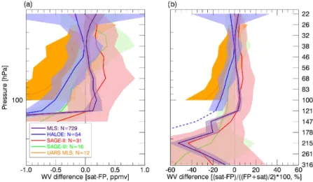
stratosphere. At lower levels (higher pressure), the satellite biases generally become larger and drier relative to the FP data.
As can be seen in Fig. 3, HALOE data are extremely dry biased (values <50 % of the FP data) below 147 hPa. This
extreme dry bias occurs because HALOE retrieval “satu-rates” under tropospheric conditions when the WV values are above ∼10 ppmv. The 147 hPa level is a transition re-gion in water vapor where the values can range from tropo-spheric to stratotropo-spheric, depending on season and latitude.
This is reflected in the HALOE/FP comparison at 147 hPa (not shown): HALOE data show mean dry biases ∼50 % when FP values are greater than 8 ppmv, as opposed to a ∼10 % dry bias for values less than 8 ppmv. To avoid a (dry) biased monthly mean from HALOE, we exclude HALOE data at and below the 147 hPa level.
The agreement between the SAGE instruments and the FP data is not as well constrained due to the small number of matches (N∼20, with even fewer matches at the lowest
Figure 3.The difference as a function of height between matched satellite and balloon frost point (FP) hygrometer water vapor (WV) data, expressed(a)as a mixing ratio difference and(b)as a percent difference between the mean value at each level (see discussion in Sect. 3.1). The number of matches at 82 hPa is shown in the legend, and the mean difference (solid) and±2 standard error (2σ/√N) range (shaded) are shown at each level. The dashed blue line shows the HALOE data that are excluded from SWOOSH, at and below 147 hPa.
200 hPa, possibly due to O3interference in the retrieval
al-gorithm (Damadeo et al., 2013). SAGE III also shows a dry bias relative to FP data, but it is within 20 % of the FP above 215 hPa.
At and above 121 hPa, Aura MLS data are within 7 % of the FP values, in broad agreement with previous findings (Lambert et al., 2007; Read et al., 2007; Hurst et al., 2014; Vömel et al., 2007a). At lower levels, the Aura MLS data ex-hibit a dry bias that varies with pressure and peaks at 36 % at 215 hPa. Our result at this level is similar to the estimated 25 % bias given in Read et al. (2007) and 27 % given by Vömel et al. (2007a) and is further explored in Appendix A. At all levels the Aura MLS and FP measurements are well within 2 standard deviations (2σ) of their mean difference
at the given level. A more rigorous metric, used in Fig. 3, is the standard error of the mean differences (σ/√N), with N adjusted to account for autocorrelation as in Santer et
al. (2000). For the null hypothesis that the measurement (i.e., population) means are equal and no systematic uncertainty exists in either measurement, the mean difference between the measurements (i.e., the sample mean difference, X) is t distributed. Then, the null hypothesis can be rejected if X > tcrit√σ
N, where tcrit≈2 (two-tailed, p=0.05). Hence, in Fig. 3 the levels at which the 2σ/√N shading intercepts
zero can be said to be in agreement with the FP data. It is worth noting that in Fig. 3 we define the per-cent difference of the satellite data relative to the mean value of the satellite and FP data (i.e., percent differ-ence=(sat−FP)/((sat+FP)/2)·100). If the percent
dif-ference is defined relative to the FP only (i.e., (sat-FP)/FP·100), there is an asymmetry whereby the percent
difference is constrained to be≥ −100 % (since WV values are constrained to be positive) but is unconstrained in the
pos-itive direction. Computing the percent change relative to one of the instruments causes the distribution of percent differ-ence at each level to be non-normal and skewed toward pos-itive values, and thus it produces pospos-itively biased estimates of the mean.
The difference in results from these two definitions is greatest below 100 hPa, where there is inherently greater variability in WV and a greater likelihood of mismatched profiles. In that region, it is much more likely that one of the pair of “matched” profiles is of dry stratospheric air and the other is of wet tropospheric air. Also, all satellites considered here have a large horizontal footprint (∼hundreds of kilome-ters) compared to the FP measurements, so this could add to the observed differences. In this region, the mean and median percent differences are very different from one another (of-ten over∼50 %) for the conventional definition (i.e., (SAT-FP)/FP·100) but are almost the same using the definition
implemented in Fig. 3.
It is clear that at many levels neither the Aura MLS nor the other satellite instruments are in agreement with the FP data, as defined by the 2σ/√N criteria. However, there are
Table 3.Ozonesonde stations used in satellite ozone comparison.
Station Latitude Longitude No. of soundings Period
Alert (CAN) 82.5 −62.3 1028 1987–2011
Resolute (CAN) 74.7 −95.0 885 1978–2011
Uccle (BEL) 50.8 4.4 2299 1996–2013
Boulder (USA) 40.0 −105.3 698 1991–2015
Wallops (USA) 37.9 −75.5 1779 1970–2013
Hilo (USA) 19.4 −155.0 1717 1982–2013
Natal (BRA) −5.5 −35.3 661 1979–2013
Samoa (USA) −14.2 −170.6 992 1995–2013
Lauder (NZL) −45.0 169.7 1275 1986-2008
Davis (ATA) −68.6 78.0 270 2003–2013
Neumeyer (ATA) −70.7 −8.3 1553 1992-2015
because the data set has been extensively validated and con-tains a relatively small mean bias over a wide range of pres-sure levels. However, it is clear that there is a significant Aura MLS UTLS dry bias at and below 147 hPa. Additional screening of the Aura MLS data set to remove low-biased WV data in the UTLS is discussed in Appendix A.
3.2 Ozonesonde comparisons
Here, we use ozonesonde data from a subset of 11 stations with high-quality measurements spanning a broad range of latitudes. These 11 stations are listed in Table 3, and their data were obtained from the World Ozone and Ultraviolet Radiation Data Centre (WOUDC) and Southern Hemisphere ADditional OZonesondes (SHADOZ) project (Thompson et al., 2012). The criteria chosen for these stations are that all stations use the electrochemical concentration cell (ECC)-type ozonesondes and provide a data record that extends back to the start of the SAGE II record in 1984. At some sta-tions ozonesonde types have been changed over the years, but only ozone profiles obtained with ECC sondes were used for the comparison here, as they have a documented accu-racy of 5–10 % below 30 km (Smit et al., 2007). Addition-ally, the sounding stations were selected to cover the polar regions and the midlatitudes of both hemispheres, as well as the tropics (see Table 3).
The temporal/spatial match criteria, outlier screening, and vertical smoothing used are the same as for the FP hygrom-eter comparison. In addition, we manually filter out obvious outlier sonde profiles with unphysical values that were not properly quality controlled and apply an additional outlier-screening algorithm that consists of removing ozone concen-trations falling 2σ outside of the mean value for each month
and each station on a 0.25 km vertical grid.
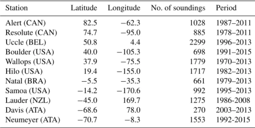
The resulting vertical profile of differences between the satellite data and ozonesondes is shown in Fig. 4. In gen-eral, the agreement between satellite and ozonesonde data is much better than for the corresponding water vapor com-parison, with all instruments falling within ±20 % of the
ozonesonde data above 100 hPa. Overall, SAGE II shows the best comparison with the ozonesonde data over the range of the stratosphere, and most of the instruments diverge from the ozonesonde data in the UTLS region around 200 hPa. For this reason, we use SAGE II as our reference ozone measure-ment to which other ozone measuremeasure-ments are adjusted.
4 Data set construction
In this section, we describe the methodology for homoge-nizing, gridding, and merging the satellite data to create the combined SWOOSH data product. Briefly, the homogeniza-tion process involves adjusting data from the individual satel-lite instruments such that their mean values agree with the reference satellite (i.e., SAGE II for ozone and Aura MLS for WV). After the homogenization process, data from each instrument are gridded individually, and the individual fields are merged into the combined product.
Figure 4.The difference as a function of height between matched satellite and ozonesonde observations. The number of matches at 82 hPa is shown in the legend, and the mean difference (solid) and±2 standard error (2σ/√N) range (shaded) are shown at each level.
measurements does not diminish because it is related to a fundamental difference in the measurements.
In SWOOSH, pairs of matched measurements between the reference satellite and the non-reference satellite are used to calculate the mean offset of the non-reference data for its full measurement period. This instrument offset is then added to the non-reference satellite data to achieve statistical agree-ment with the reference data.
The matching methodology for the inter-satellite matches is the same as in Sect. 3 for the comparison between balloon sounding data and satellite data. Because of the relatively sparse sampling of the solar occultation measurements, we use the less strict criteria described in Sect. 3: specifically, we use the pair of measurements with closest equivalent lati-tude that is within±2 days,±2000 km E–W distance (±18◦
longitude at the Equator), and±1000 km N–S distance (±9◦ latitude) from one another. With these criteria, the number of matched pairs ranges from ∼5000 to 25 000 depending on the specific combination of instruments.
The matching between the reference and non-reference data set for each species is possible for all combinations of data sets except between Aura MLS and UARS MLS for wa-ter vapor, since their records do not overlap. In the absence of instrument overlap for these two instruments, we use the (adjusted) HALOE WV as a transfer standard.
After matching, we interpolate all satellite data onto the SWOOSH vertical grid, which corresponds to the Aura MLS vertical grid containing 12 levels per decade in pressure from 316 to 1 hPa. This grid is coarser than the retrieval vertical grids of all of the other instruments except for UARS MLS, which has roughly half the number of vertical levels as Aura MLS.
It is worth noting that the vertical resolutions of the satel-lite instruments are not the same and range from about 1 to 5 km depending on the species, instrument, and vertical
level considered (see Table 1). We conducted tests smooth-ing the higher-resolution data down to the∼3 km resolution of Aura MLS and did not find large changes in the computed offsets, even near the tropopause, indicating that the offsets are caused more by fundamental retrieval issues than simple differences in vertical resolution of the measurements. For simplicity, we use linear interpolation in log-pressure space to put all satellite data sets on the Aura MLS levels. Satel-lite data sets on a native altitude–number-density coordinate system (i.e., SAGE II and SAGE III) have all been converted to pressure-mixing ratio coordinates using temperatures from the MERRA reanalysis.
After matching and interpolating to a common vertical grid, the mean offset is calculated for each vertical level and 10◦latitude bin for each combination of satellite instruments.
Figures 5 and 6 show the offsets as a function of height and latitude for water vapor and ozone, respectively. It is worth stressing that the offsets added to the non-reference satellite data here do not vary with time or season, only with height and latitude. Thus, drifts or other unphysical changes in indi-vidual satellite records, if they exist, are not accounted for in SWOOSH.
In addition to the instrument offsets, we also compute the uncertainty in the offsets. Since the offset is defined as the mean difference between coincident pairs of satellite instru-ments within a 10◦latitude bin at a given pressure level, the
offset uncertainty is simply the standard error of this mean difference (i.e.,σ/√N). This is illustrated in Fig. 7, which
shows the 68 hPa level offset vs. latitude for HALOE/Aura MLS and the histogram of mean difference between the two at one latitude band.
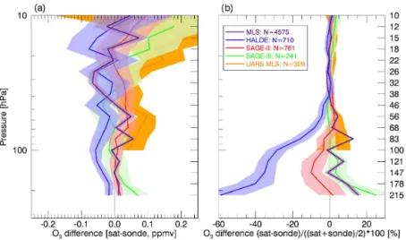
ho-Figure 5.WV offsets relative to Aura MLS for satellite data sets used in SWOOSH. WV offsets are defined as the mean of MLS minus the given data set. Offsets are computed on the MLS vertical grid in 10◦latitude bands.
Table 4.Available SWOOSH grids.
Longitude Latitude Vertical type
– 2.5, 5, or 10◦ Pressure – 2.5, 5, or 10◦ Isentropic
20◦ 5◦ Pressure
30◦ 10◦ Pressure
mogenization process to illustrate the magnitude of the off-sets and their uncertainty.
4.2 Gridding
SWOOSH is produced on several different horizontal and vertical grids to serve different user needs. For a given hor-izontal/vertical SWOOSH grid (summarized in Table 4), the data from all species and satellites are stored in a single file with a monthly time resolution. On each horizontal grid for each species/satellite/month, SWOOSH contains several dif-ferent monthly statistics, including the mean mixing ratio for both the “raw” and “adjusted” versions of the data, the num-ber of profiles, their standard deviation, and a measure of the combined retrieval (precision) and offset uncertainties.
The uncertainties stored in SWOOSH for each species are the root-mean-sum-of-squares (RMSS) combination of the retrieval precision uncertainty and offset adjustment uncer-tainty. A derivation and description of the SWOOSH source record uncertainty estimates is provided in Appendix B.
Figure 6.Same as Fig. 5 but for O3offsets, which are relative to the SAGE II data.
The primary SWOOSH grid is a zonal-mean gridded data set (either 2.5, 5, or 10◦latitude) on pressure levels (12
lev-els per decade from 316 to 1 hPa, corresponding to the Aura MLS pressure levels). The three different resolutions of the zonal-mean grids are provided to satisfy different user needs. In general, the finer-resolution grid will be noisier and con-tain more missing data. However, as each unique grid reso-lution is computed independently, the uncertainty estimates (discussed in Sect. 4.4) reflect the different sampling. Al-though data at pressure levels above 1 hPa are available in most of the source data sets used in SWOOSH, the ampli-tude of the diurnal cycle in ozone is largest above this level. However, studies have shown diurnal variability of about 5– 10 % in the uppermost stratosphere and the SWOOSH record makes no attempt to quantify biases that may be related to diurnal sampling or to non-uniform spatial or temporal sam-pling within a monthly latitudinal grid box. Depending on the magnitude of the seasonal or sub-monthly gradients, uneven sampling could introduce additional systematic error beyond what is accounted for in the SWOOSH uncertainty estimates (Damadeo et al., 2014; Neely et al., 2014).
Figure 7.Example of WV offset adjustment for HALOE at 68 hPa.(a)Matched MLS/HALOE pairs (dots), the 10◦latitude binned means (red filled triangles) with error bars showing the offset uncertainties (95 % confidence interval). The mean (over all latitudes) is shown as a horizontal blue dashed line.(b)The histogram of MLS/HALOE differences at 68 hPa for the 40–30◦S latitude bin. The offset uncertainty for this bin is shown as a horizontal red bar.
Figure 8.Top: the uncorrected source water vapor time series in the 30–40◦S latitude band at 68 hPa, along with the source standard de-viation (sk, wide error bars) and root-mean-sum-of-squares (RMSS) uncertainty values (σrmssk, narrow error bars). Bottom: the offset-corrected source measurements along with the combined (“anomaly filled”) product. The lighter and darker gray shaded regions show the combined RMSS uncertainty (σrmss, dark gray) and the com-bined standard deviation (s, light gray), respectively. The vertical error bars in the lower panel show the 95 % confidence interval of the offset uncertainties for the 30–40◦S latitude band at 68 hPa.
For the zonal-mean SWOOSH grids, SWOOSH variables are provided on an equivalent latitude grid (in addition to the standard geographic latitude grid). Here, equivalent lat-itude is defined using PV on an isentropic (θ) surface, as
used in numerous previous studies (e.g., Nash et al., 1996; Butchart and Remsberg, 1986). Briefly, at a given location the equivalent latitude is defined as the latitude for which
Figure 9.Same as in Fig. 8 but for ozone.
the area poleward is the same as the area of the PV contour at that location. Compared to a geographic latitude coordi-nate system, long-lived tracers such as WV/O3in a PV-based
equivalent latitude coordinate system contain less variability, as north–south excursions in the tracer field are due to largely reversible synoptic-scale features.
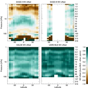
Figure 10.Ozone height vs. latitude plots on geographic latitude (left column) and equivalent latitude grids (right column), for Octo-ber 2004. Increased data coverage and increased depth of Antarctic ozone depletion are apparent in the equivalent latitude gridded data.
clearer on an equivalent latitude grid than on a geographic latitude grid. Also, at many levels improved horizontal cov-erage is achieved on the equivalent latitude grid relative to the geographic grid. Outside of the vortex and the subtrop-ical tropopause region, the equivalent latitude gridded data are very similar to the geographic latitude gridded data, as expected. The similarity between these two grids is exploited in Sect. 4.5 to use the equivalent latitude gridded data to fill in data missing from the geographic grid.
4.3 The combined monthly-mean product
After all of the individual satellite data sets have been offset-adjusted and gridded, the combined SWOOSH prod-uct is formed from the source data records. For a given month/latitude/level, data from all available satellite instru-ments are combined using a weighted average based on the number of observations from each instrument, i.e.,
q=
K X
k=1
qk Nk Ntot,
whereqkis the monthly-mean mixing ratio of thekth satellite
in the bin,Nkis the number of observations in the bin,Kis the number of satellites, andNtot=
K P
k=1
Nk.
By combining data in this way, the combined product is dominated by the Aura MLS measurements after their intro-duction in August 2004, as Aura MLS contains more than an
order of magnitude more data in a monthly grid box than all of the other data sets combined. In the pre-Aura MLS period the data density is often low for a single instrument in a given 10◦latitude band, so combining data using a weighted mean
based on the number of available measurements (rather than simply averaging the two monthly means, for example) gives a more representative value.
We note that there are a number of alternative methods for creating a merged and gridded data set (Randel and Wu, 2007; Froidevaux et al., 2015). In particular, one method of creating a merged data set is to merge the source record anomalies rather than the absolute values. In this case, the anomalies may be adjusted so that their mean difference is zero during the overlap period. One advantage of this ap-proach is that any unphysical differences in the seasonal cy-cles between two instruments are removed by only consid-ering their anomalies. However, since a seasonal cycle must be imposed in order to convert back to physical mixing ra-tio values, this approach implicitly removes any long-term changes in the seasonal cycle between two instruments. Fur-thermore, it can be shown that this approach is equivalent to applying a seasonally varying offset adjustment, which in-flates the degrees of freedom by a factor of 12 compared to the standard approach applied in SWOOSH. We note that in SWOOSH the necessary information (e.g., mean values,
N, uncertainties, individual instrument anomaly records) is
stored for each of the satellite source records for users to be able to create and explore alternative methodologies for combining the satellite products, based on “anomaly match-ing” or other methods. It is also possible to implement the SWOOSH combined product definition outlined above with subsets of the available satellite data (e.g., with just HALOE and Aura MLS).
4.4 Uncertainty in the combined monthly-mean product In addition to the combined monthly means, an uncertainty and standard deviation of the combined product is also pro-vided in SWOOSH. The derivation and details of the com-bined uncertainty and standard deviation estimates are pro-vided in Appendix B, as well as an explanation of the mean-ing of the terms in the combined uncertainty and standard deviation estimates. In this section, we provide an overview of the uncertainty and standard deviation estimates that are derived and described in detail in Appendix B, along with examples and discussion of their use in SWOOSH.
As shown in Appendix B, the uncertainty forkth satellite’s
monthly-mean value (σqk) can be expressed as a standard er-ror of the mean
σqk=
σrmssk √
Nk
,
vidual satelliteσrmssk values,
σRMSS=
v u u t
K X
k=1
σrmss2
k
Nk
Ntot, (1)
weighted by the number of measurements Nk for a given satellite in that months lat/height bin.
Also stored is the standard deviation of the source mea-surements contributing to the monthly mean (sk) as well as a
standard deviation for the combined product (s). Figures 8
and 9 illustrate the individual satellite standard deviations and RMSS uncertainties, the combined RMSS uncertainty, the combined standard deviation, and the offset uncertainties. One issue that stands out in these figures is that while the individual satellites have quite similar standard deviations to one another, their retrieval uncertainty estimates vary wildly, particularly for water vapor. For example, the HALOE WV uncertainties are extremely small relative to the other instru-ments, whereas the SAGE II WV uncertainty estimates are relatively large. Furthermore, the HALOE (WV) uncertain-ties are much smaller than the corresponding HALOE stan-dard deviations, and the SAGE II uncertainties are larger than the SAGE II standard deviation by a factor of∼3 (see dis-cussion below).
It is worth noting that in general, the “observed” standard deviations (sk) should be of similar magnitude or greater than the instrument precision uncertainty (i.e., the random uncer-tainty). For example, if geophysical variability (i.e., the pop-ulation standard deviation for a given height/latitude/month bin) is small relative to the instrument uncertainty, then the observed (sample) standard deviation should be close to the instrument uncertainty. If, however, geophysical variability is larger than the instrument uncertainty, then the observed standard deviation is a mixture of both instrument precision and geophysical variability.
For the case of water vapor at the 68 hPa level illustrated in Fig. 8, the Aura MLS WV monthly precision uncertain-ties and standard deviations are of the same magnitude. This result is consistent with Lambert et al. (2007), who demon-strated that the “observed” and “expected” (i.e., based on in-strument precision) standard deviations of coincident pairs
icant O3variability.
The mismatch of the WV instrument uncertainties and standard deviation in SAGE II and HALOE data has impor-tant implications for the combined uncertainty estimates in SWOOSH. It is possible that the HALOE uncertainties are underestimated and it is likely that the SAGE II uncertain-ties are overestimated, which leads to an artificially inflated or deflated SWOOSH combined WV uncertainty estimate before August 2004, depending on which instrument con-tributes more data to a given lat/month/height bin. As dis-cussed in Damadeo et al. (2013), the most likely explanation for the overestimated SAGE II uncertainties is the inclusion of additional aerosol clearing uncertainty, which inflated the water vapor uncertainty. Because of these issues with indi-vidual satellite record uncertainties and their knock-on ef-fects on the combined uncertainty estimates, users may wish to use the combined standard deviation (s, Eq. B16) for a
wa-ter vapor uncertainty estimate during the pre-Aura MLS pe-riod instead of the combined uncertainty value (σq, Eq. B7).
4.5 Additional SWOOSH products: climatology, anomaly, and filled data
Depending on the scientific objectives, it is desirable, or in-deed required in some cases, to have a data set that is free of missing data. In other cases, the focus may be the climato-logical seasonal cycle or departures from the seasonal cycle (anomalies). SWOOSH includes several data products to ful-fill these needs.
For most variables including the individual satellite data and the combined product, there is both a seasonal cycle and an anomaly time series provided. The anomaly time series simply has the long-term mean seasonal cycle (computed over the entire record) removed at each time/grid box.
samples between 82◦S and 82◦N, so any grid boxes
pole-ward of these latitudes would contain no data in the geo-graphically gridded version of the variables. However, in any given month, Aura MLS typically samples air masses with an equivalent latitude poleward of 82◦, as reflected in the
equivalent latitude gridded version of the data in Fig. 10. It is worth noting as a warning to users that in the exam-ple of polar ozone loss this filling is likely to add values in that are an underestimate relative to the true geographical zonal means, because inside the polar vortices the ozone at a given equivalent latitude is less than the corresponding geo-graphic latitude. However, at other latitudes and for water va-por where the geographic and equivalent latitude latitudinal distributions are similar, the procedure does not introduce a significant bias. Other than at the most poleward grid points, the equivalent latitude filled combined product is only sig-nificantly different than the regular combined product in the pre-Aura MLS period when there are large (latitudinal) gaps in the data in any given month.
In addition to the equivalent latitude filled version of the data, which in general is not a gap-free data set, SWOOSH also includes an anomaly filled version of the data (see Fig. 11) that is free of missing data. In this version, the anomaly data (Fig. 11b) are first filled in the latitude–time plane (separately at each vertical level) using radial basis function interpolation with an inverse multiquadric function (Fig. 11c). In such an interpolation, the interpolated value is based on a mean of nearby points weighted by the in-verse of their distance (Hardy, 1990). In the SWOOSH pro-cessing, this is implemented using the Interactive Data Lan-guage (IDL) GRIDDATA routine with the default radial ba-sis function settings. Because the poles contain missing data throughout the record, we fix the anomaly values at zero at the poles. Doing this ensures that the anomaly filled field will relax towards zero from the most poleward valid value in the anomaly field. After this step, the anomaly array (Fig. 11c) is simply added back to the corresponding seasonal cycle ar-ray to produce what is known as the combined anomaly filled version of the SWOOSH data (Fig. 11d).
As a final note, we stress that the anomaly filled version of the SWOOSH data represents only one way of creating a filled data set; where trend analysis is of interest the unfilled version of SWOOSH should be used for analysis, partly out of caution and partly because it contains reliable uncertainty estimates that can be used for trend uncertainty estimation. The anomaly filled data should in general be used with ex-treme caution in the pre-1990 time period. Regions with very sparse and noisy data can have undue influence over large re-gions in the filling process, as can be seen in the high south-ern latitudes in the example shown in Fig. 10b–c.
Figure 11.(a)Combined (unfilled) latitude vs. time cross section of WV at 68 hPa.(b)The anomaly of(a), defined as(a)minus the seasonal cycle at each latitude.(c)A filled version of(b), using ra-dial basis function interpolation.(d)The combined (anomaly filled) product, which is constructed by adding the (latitude-dependent) seasonal cycle to the filled anomaly(c).
5 Examples of variability and comparison to independent observations
In this section, we demonstrate the utility of SWOOSH for quantifying and studying seasonal and interannual variabil-ity in stratospheric water vapor and ozone. SWOOSH is used to illustrate several well-known ozone and water vapor phe-nomena such as the tropical tape recorder, transport of ozone and WV anomalies in the lowermost stratosphere, and vari-ability related to the quasi-biennial oscillation (QBO). These phenomena can generally be captured by a single satellite record, but the combined SWOOSH record allows for the study of variability on longer timescales.
nal from the individual satellite instruments, as well as the combined anomaly filled SWOOSH product, and the trop-ical tape recorder anomaly. As can be seen from this plot, the combined data clearly capture the post-2000 drop in WV, as well as significant interannual variability. Using the com-bined product, we compute the post-2000 drop in water vapor to be 0.4 ppmv (averaged 30◦S–30◦N; June 2001–June 2005
minus 1996–2000), similar to the values found in other stud-ies (e.g., Randel et al., 2006; Solomon et al., 2010).
Similar to the tape recorder plot, Fig. 13 shows the deep tropics (10◦S–10◦N) averaged ozone anomalies as a
func-tion of height and time. The descent of ozone anomalies associated with the QBO can be clearly seen in this figure. Numerous studies have identified QBO-related variations in ozone concentration and column amount (e.g., Angell and Korshover, 1964, and references therein; Oltmans and Lon-don, 1982; Zawodny and McCormick, 1991; Randel and Wu, 1996). In Fig. 14, we show a comparison between the 56 hPa combined zonal-mean SWOOSH ozone product and the ozonesonde record from Natal, Brazil (5◦S, 35◦W), that
was included in the ozonesonde comparison in Sect. 3. This station is the only station from that data set that lies within the deep tropics where QBO-related variations in ozone occur. As can be seen in Fig. 14, the comparison between SWOOSH and the ozonesonde record at Natal is quite good. The com-parison period covers a time period when HALOE, SAGE II, and Aura MLS contribute to this tropical latitude band. For the most part the error bars from the Natal data overlap the SWOOSH record, and in all cases they overlap with the stan-dard deviation within the 10◦latitude band.
5.2 Interannual anomalies in transport of ozone and water vapor
In this section, we illustrate the utility of SWOOSH for cap-turing interannual anomalies in WV/O3 that are related to
transport in the lower stratosphere. Figure 15 shows the lat-itude vs. time cross sections of WV/O3anomalies at 82 hPa
in the lower stratosphere. By removing the seasonal cycle, the poleward transport of tropical WV anomalies is easily seen (Fig. 15a), as are interannual variations (e.g., related to the QBO or El Niño–Southern Oscillation, such as the large
Figure 12.The tropical average (30◦S–30◦N) water vapor con-centration as a function of height and time, which is commonly re-ferred to as the “tropical tape recorder”, for each satellite data set in SWOOSH(a–d), as well as the two combined products(e–f)and the combined (filled) anomaly product(g). SAGE III data are non-existent in the tropics and therefore not included.
El Niño event at the end of 2015). For ozone, the interan-nual variations in anomalies related to interaninteran-nual variations in polar ozone loss can be seen (Fig. 15b). For example, the weak Antarctic ozone depletion in 2012 (Klekociuk et al., 2014) can easily be seen, as can the severe Arctic polar ozone loss in 1993 (Larsen et al., 1994), 1995 (Manney et al., 1996), and 2011 (Manney et al., 2011).
5.3 Comparison to the Boulder frost point hygrometer record
Here we compare the SWOOSH merged record with the NOAA FP hygrometer record from Boulder, Colorado (40◦N, 105◦W); this is the only long-term in situ record of
stratospheric water vapor (dating back to 1980) that covers the entire SWOOSH time period. Indeed, the lack of any additional long-term records was a primary motivating fac-tor for the construction of the SWOOSH data set. Figure 16 shows the SWOOSH combined product at 68 hPa (35◦N–
Figure 13.The tropical average (10◦S–10◦N) ozone concentration anomaly as a function of height and time for each satellite data set in SWOOSH(a–d), as well as the two combined products(e–f).
from 80 to 56 hPa (roughly 2.5 km centered on 68 hPa). The error bars plotted in this figure for the FP data are twice the standard error within the layer average. For SWOOSH, the shaded region is 2 standard deviations of the combined prod-uct (Eq. B16). Although the SAGE II measurements began in 1984, there are no data at this level and latitude band un-til 1988 due to aerosol contamination from the El Chichón eruption.
As can be seen from this figure, the variability of the SWOOSH zonal-mean combined product and the Boulder record overlap one another for most of the period, with the exception of the beginning of the SWOOSH record when the only available satellite data was from SAGE II. Reasons for this difference are worthy of further exploration, and this per-haps points to a drift in the in an individual SAGE II satellite record that the SWOOSH data merging technique does not consider (Damadeo et al., 2013; Thomason, 2004). Differ-ences between the long-term in situ FP record and certain satellite records have been noted previously (e.g., Hegglin et al., 2014; Kley et al., 2000). Aura MLS was chosen as the ref-erence water vapor measurement because it agreed best with the FP data. If a different reference satellite was chosen, it would change the effective offset from the FP measurements
but not alter the long-term trend. There are clearly differences between the long-term trend derived from the satellite water vapor measurements and that from midlatitude in situ mea-surements (Hurst et al., 2011; Kley et al., 2000; Oltmans and Hofmann, 1995; Oltmans et al., 2000; Rosenlof et al., 2001); such differences still exist when comparing to the SWOOSH data set.
6 Discussion
For understanding interannual to decadal variability in the ra-diatively important trace species of water vapor and ozone on a global scale, it is necessary to combine data records from satellite measurements made with different measurement techniques, data densities, and resolutions. In this paper, we have documented the construction of a new vertically re-solved data record of ozone and water vapor from limb mea-suring satellites. The SWOOSH method of combining lite data records involves adjusting the non-reference satel-lite data sets relative to a reference satelsatel-lite record through the application of offsets. The offsets that are applied to the non-reference data are allowed to vary as a function of lat-itude and height, but not temporally, to allow for the possi-bility that inter-satellite biases vary spatially, and are based on coincident pairs of vertical profiles taken during instru-ment overlap time periods. The choice of a reference satel-lite data set is justified based on the best agreement with independent balloon-based sounding measurements so that the SWOOSH combined values will agree with the balloon measurements in an average sense. The adjustment method used in SWOOSH is conceptually similar to previously used methods for combining satellite data sets (Randel and Wu, 2007; Froidevaux et al., 2015) except that merging is done to a reference instrument and takes place in absolute value space rather than in anomaly space, for the reasons noted above.
It must be stressed that no attempt is made to correct for potential satellite drifts in SWOOSH. In principle it is pos-sible that satellite drift could be accounted for by correcting the individual source record or by applying a time-varying offset adjustment to the data. However, currently the abil-ity to assess and construct time-varying corrections for these data is limited due to the sparse sampling of the solar occul-tation satellites used in the pre-2004 period and the limited spatial and temporal availability of high-quality in situ mea-surements for comparison (Hurst et al., 2016; Hubert et al., 2016).
nec-Figure 14.The Natal, Brazil (5◦S, 35◦W), ozonesonde monthly means in a 2 km layer centered on 56 hPa (purple triangles). Error bars show the 95 % confidence interval for the ozonesondes data. Also shown are the SWOOSH combined O3zonal-mean data for the 10–0◦S band. The light gray shading is twice the SWOOSH combined standard deviation product described in the text.
Figure 15. SWOOSH combined product water vapor and ozone anomalies (unfilled) at 82 hPa.
essary data are saved to investigate alternative combinations of the data sets (e.g., excluding one of the satellites).
The SWOOSH record constitutes a unique tool for study-ing interannual to decadal-scale variability in water vapor and ozone. The documentation of data provenance, filtering, and merging methodology presented here provides a trace-able basis for future intercomparison studies addressing the agreement of satellite data with balloon and/or ground-based measurement systems, and it will be useful for sensitivity studies addressing the impact of satellite homogenization methodologies. The SWOOSH record may prove useful as
input to global models lacking interactive ozone chemistry, and will likely be useful for future studies to quantify the radiative impact of water vapor and ozone variability in the UTLS region. Based on the data presented here, we offer a set of recommendations for users of SWOOSH data.
The unfilled version of the combined SWOOSH data set should be used where possible, especially for trend studies, to avoid potential biases introduced in the filling process and also because uncertainty estimates are provided.
Users should be aware that large data gaps in space and time exist in the early part of SWOOSH, particularly for wa-ter vapor before the early 1990s. Studies using the SWOOSH anomaly filled data set should exercise extreme caution in using the data during these time periods. Regions that have been filled can be identified either by directly comparing the anomaly filled arrays to the corresponding non-filled version or by considering theN arrays (arrays containing number of
data points that went into the bin).
Data below 100 hPa are extremely limited, and users should exercise additional caution when analyzing data in this region.
The SWOOSH data (version 2.5) used in this paper are publicly available through the end of 2015 through the NOAA data catalog at https://data.noaa.gov/dataset/stratospheric-water-and-ozone-satellite-homogenized-swoosh-data-set. The SWOOSH data will continue to be updated as long as new data are available from the Aura MLS instrument or a suitable replacement.
Figure 16. The SWOOSH combined (unfilled) record at 68 hPa and 35–45◦N (black line) along with the Boulder NOAA frost point hygrometer record averaged from 80 to 56 hPa (purple diamonds). Error bars for the Boulder data are 2 standard errors (∼95 % confidence
interval) of the mean within the layer, and the shaded area for SWOOSH shows twice the standard deviation of the combined (unfilled) product. The unadjusted satellite source record time series at 68 hPa and 35–45◦N are also shown (colored lines and squares).
record. This measurement will continue with the launch of Joint Polar Satellite System (JPSS)-2.
In contrast to ozone, currently Aura MLS is the only ver-tically resolved stratospheric water vapor data set capable of providing global coverage for input to the SWOOSH record. In the near future, there are plans to deploy a SAGE III in-strument on the International Space Station that will be ca-pable of providing vertically resolved water vapor, but with severely reduced sampling compared to Aura MLS. Given the water vapor offsets between the satellite instruments demonstrated here, the potential data gap in the water va-por record would severely impact our confidence in charac-terizing decadal variability and trends in water vapor. As dis-cussed by Müller et al. (2016) and demonstrated in this paper, it is possible that a global network of balloon-borne hygrom-eter measurements could help serve as a transfer standard be-tween satellites and minimize the impact of a potential water vapor data gap in the satellite record.
7 Data availability
Finland (67◦N), on 7 March 2008. The 15 closest Aura MLS
profiles that meet the match criteria described in Sect. 3.1 are shown in the figure. The upper two plots in Fig. A1 illus-trate that the Aura MLS measurements undergo an oscillation about the FP profile in the UTLS region between∼316 and 100 hPa, with local minima at 215 hPa and local maxima at 147 or 121 hPa.
The oscillation is apparent in the Aura MLS a priori pro-files (Fig. A1c). These a priori propro-files are a result of three separate retrievals that are constrained to be piecewise con-tinuous at 147 and 316 hPa (Read et al., 2007). The exis-tence of the oscillation in both the a priori profiles and the retrieved profiles suggests that the oscillation is not simply an artifact caused by the Aura MLS vertical averaging ker-nel being applied to a region of high vertical WV gradients but rather is introduced at the a priori retrieval stage. To con-firm this, we used the Aura MLS averaging kernel to degrade the high-resolution CFH data to the Aura MLS levels using the method described in Read et al. (2007), and we found that this process does not introduce an oscillation to the CFH data (Fig. A1d).
Since the procedure for applying the Aura MLS averaging kernel to an FP profile requires as input an a priori profile, we also tested the sensitivity of our results to the use of different a priori profiles by using both the Aura MLS a prioris and the CFH profile as the a priori input. Even when the Aura MLS a priori profiles containing a UTLS oscillation are used as the a priori input to the smoothing procedure, the output CFH profiles do not contain a large oscillation. This is not surprising given that the integrated averaging kernels at these levels are near unity, implying that retrieved WV values at these levels come from the Aura MLS measurements and not the a priori.
To establish that the Aura MLS dry bias is a significant feature from a monthly-mean and climatological perspective, Fig. A2 shows a zonal-mean cross section of water vapor from the Aura MLS, Aura High Resolution Dynamics Limb Sounder (HIRDLS version 7; Khosravi et al., 2009), UARS HALOE, SAGE II, SAGE III, and ACE-FTS version 3.5 (Bernath et al., 2005) satellite data for the month of March. The dry bias at 215 hPa identified above is obvious in the zonal-mean monthly-mean Aura MLS data at high latitudes.
here asq) at either 121 or 147 hPa. Quantitatively, we define
these data artifacts as
121 hPa oscillation: q261> q215< q177
andq147< q121> q100
147 hPa oscillation: q261> q215< q177
andq178< q147> q121
121 hPa spike: q147< q121> q100
and 121 hPa oscillation conditions not met 147 hPa spike: q178< q147> q121
and 147 hPa oscillation conditions not met.
Figure A3 shows the Aura MLS-FP comparison as in Fig. 3, but broken up by the four types of spikes/oscillations identi-fied above. As can be seen in this figure, the two oscillation types contain extremely dry-biased conditions at 215 hPa. In contrast, the local maxima at 121or 147 hPa are wet biased relative to the FP data.
As can be seen in Fig. A3, the Aura MLS data are biased at and below the level of the local maximum in the four types of features. For example, for Aura MLS profiles containing the 121 hPa oscillation (i.e., yellow dashed line in Fig. A3), the data at and below 121 hPa appear to be problematic, whereas the upper part of the profile looks similar to Aura MLS pro-files that do not contain an oscillation/spike feature. Because the Aura MLS profiles appear relatively unaffected at the higher levels when the data artifacts are present at the lower levels, we filter the data by simply removing the part of the profile below the local maximum (i.e., at 121 or 147 hPa).
At some latitudes and during some seasons, this removes a significant fraction of Aura MLS data below 100 hPa. Fig-ure A4 illustrates the occurrence frequency of the four types of UTLS features found in Aura MLS data, binned into 10◦
latitude bins by month. As can be seen in this plot, the data artifacts occur in more than 50 % of Aura MLS profiles for most of the year at latitudes poleward of 50◦latitude in each
hemisphere.
at high pressures with the Aura MLS instrument, as mani-fested in the a priori retrieval. Under these conditions, the dry continuum emission is the dominant absorber, and errors in the independent tangent pressure/temperature retrievals that are used to estimate and remove the dry continuum emis-sion could lead to “knock-on” effects in the retrieved WV. Indeed, the occurrence pattern of the data artifacts at 147 and 121 hPa (Fig. A4e–f) exhibit a pattern that looks to be related to temperatures in the UTLS (Fig. A4 g and h). In particular, the occurrence pattern at 147 hPa appears to correlate loosely with the temperature at 300 hPa (compare Fig. A4e and g), whereas the pattern at 121 hPa correlates with the tempera-ture at 150 hPa (Fig. A4f and h). Interestingly, the correla-tion patterns are reversed. The 147 hPa artifacts are antirelated with temperature; lower temperatures at 300 hPa cor-relate with a higher frequency of occurrence of the 147 hPa artifact. In contrast, the 121 hPa artifacts are positively corre-lated with temperature. The robustness and reasons for these correlations are unknown and warrant further study.
Figure A1.(a)Cryogenic Frost Point Hygrometer (CFH) H2O profile (black) taken from Sodankyla, Finland (67◦N), on 7 March 2008, along with the 15 closest-matched Aura Microwave Limb Sounder (MLS) H2O profiles (colored).(b)The difference between the matched MLS profiles and the CFH data.(c)The MLS a priori profiles corresponding to the MLS H2O retrieval values shown in the upper left panel.
(d)The CFH data averaged to the MLS resolution using different a priori profiles as input to the procedure described by Read et al. (2007). The black line is based on the CFH as the a priori, whereas the colored lines are the result of using the corresponding colored line from the lower left panel.
Figure A2.Zonal-mean height vs. latitude cross section of water vapor from six satellite instruments for the month of March, averaged from 2001 to 2009. Data are gridded on a 10◦latitude grid using PV-based equivalent latitude from MERRA.