Finite Element Analysis of Magnetic Field Distribution for 500-kV Power Transmission Systems

(1)

Abstract_{—This paper proposes a set of mathematical models} presenting magnetic fields caused by operations of an extra high voltage (EHV) transmission line under normal loading and short-circuit conditions. The mathematical models are expressed in second-order partial differential equations derived by analyzing magnetic field distribution around a 500-kV power transmission line. Finite element methods (FEM) for solving wave equations have been exploited. The modification for complex magnetic field analysis and time-harmonic simulation are also utilized. The computer simulation based on the use of the FEM has been developed in MATLAB programming environment. The problem of study is intentionally two-dimensional due to the property of long line field distribution. To verify its use, i) single-circuit and ii) double-circuit, 500-kV power transmission lines have been employed for test.From all test cases, the calculation line of 1.0 m above the ground level is set to investigate the magnetic fields acting on a humanin comparative with ICNIRP standard. Moreover, visualization of magnetic fields caused by fault currents flowing through EHV transmission lines is included.

Index Terms—Magnetic Field, Finite Element Method (FEM), Transmission Line, Short-Circuit Faults, Computer Simulation

I. INTRODUCTION

500-kV extra high-voltage (EHV) transmission lines of Electricity Generating Authority of Thailand (EGAT) have been increasingly installed due to electrical demand growth in Thailand. The first 500-kV power lines is a double-circuit configuration linked between Maemoh Power Plant, Lumpang province and Thatako Substation, Nakhon Sawan province. Another 500-kV power link is a single-circuit power transmission line connecting between Thatako Substation and Nongchok Substation, Bangkok. The impact of electric fields surrounding the transmission line depends strongly on conductor surface potentials, while load currents flowing through the transmission line result in magnetic field distribution. For the 500 kV systems, high current density transmission is the main purpose. It can cause electrical P. Pao-la-or is with the School of Electrical Engineering, Institute of Engineering, Suranaree University of Technology, Nakhon Ratchasima, THAILAND (corresponding author to provide phone: 0-4422-4400; fax: 0-4422-4601; e-mail: padej@sut.ac.th).

A. Isaramongkolrak is with the School of Electrical Engineering, Institute of Engineering, Suranaree University of Technology, Nakhon Ratchasima, THAILAND (e-mail: anone_91@hotmail.com).

T. Kulworawanichpong is with the School of Electrical Engineering, Institute of Engineering, Suranaree University of Technology, Nakhon Ratchasima, THAILAND (e-mail: thanatchai@gmail.com).

hazards to people or their livestock nearby. Especially when the power system was faulted, the short-circuit current is much higher than the normal current loading. This paper focuses on utilization of efficient computing techniques to estimate the magnetic field distribution. Obtained estimate solutions can lead to assessment of electrical hazards for 500-kV power transmission systems.

Finite Element Method (FEM) is one among popular numerical methods that is able to handle problem complexity in various forms. At present, the FEM has been widely applied in most engineering fields. Even for problems of magnetic field distribution, the FEM is able to estimate solutions of Maxwell’s equations governing the 500-kV power transmission systems. Potential and electric field analysis resulting from high voltage conductor potentials of a power transmission lines have been increasingly reported. In contrast, most of magnetic field analyses in high voltage power transmission systems focus on magnetic shielding problems [1]-[3]. There are some works studying effects of magnetic fields on environment surrounding a power line carrying high current. By literature, these research works are conducted based on electromagnetic theory or image theory [4], [5]. With defining a line of calculation and assuming very thin power lines, two-dimensional problems of magnetic field analysis governed by empirical mathematical expressions can be applied. However, these conventional methods are unable to include effects of bundled conductors that are typical for EHV power transmission systems. To provide a potential tool of simulation, the FEM is flexible and suitable to estimate magnetic field distribution. Although the conventional methods are simpler than the use of the FEM, they are limited for the system of simple geometry. In practice, several metallic structures can be found underneath the power transmission line, e.g. steel tower trusts, communication lines nearby, metallic fends or other lower voltage transmission lines. Employing the FEM can includes these effects by choosing material magnetic permeability for each additional structure domain. With this feature, the FEM is one of potential numerical simulation tools for analyzing magnetic field problems of combined material regions. Unfortunately, there is no report of exploiting the FEM for magnetic field analysis of electric power transmission systems. To utilize the advantages of the FEM for handling the magnetic field problems, FEM model development and problem formulation need to be defined in magnetic field problems of EHV power transmission systems.

Finite Element Analysis of Magnetic Field

Distribution for 500-kV Power Transmission

Systems

P. Pao-la-or, A. Isaramongkolrak, and T. Kulworawanichpong

(2)

In this paper, magnetic field modelling of power transmission lines is briefed in Section II. Section III is to illustrate the utilization of the FEM for the magnetic field modelling described in Section II. Section IV gives simulation results in both normal and faulted conditions,and discussion. Test cases given in this paper is the 500-kV transmission line that has been installed in Thailand. It is currently the highest operating voltage level in this country. The simulation conducted herein is based on the FEM method given in Section III. All the programming instructions are coded in MATLAB program environment. Moreover, due to excessive magnetic fields that might be harmful to people or livestock living nearby, careful investigation of the magnetic phenomena is taken into account. According to the standard of International Commission of Non Ionizing Radiation Protection (ICNIRP), the satisfactory simulation results are also complied with the ICNIRP standard.

II. MAGNETICFIELDMODELINGFORAPOWER TRANSMISSIONLINE

The mathematical model representing magnetic fields (B) caused by a power transmission line carrying high current is expressed in form of the magnetic field intensity (H) in which

H

B

=

μ

. Utilizing the wave equation (Helmholtz’s equation) as in (1) [6], [7], magnetic field modeling that follows the Ampere’s circuital law is defined.

0

2 2

2

=

∂

−

∂

−

∇

t

H

σμ

εμ

(1)

where

ε

is the constant dielectric permittivity,

μ

is the magnetic permeability, and

σ

is the conductivity.

This paper has considered the time-harmonic system by representing

H

=

He

jωt [8], therefore

H

j

t

=

ω

∂

H

and

H

t

2 2

2

ω

−

=

∂

H

where

ω

is the angular frequency

Therefore, refer to (1) can be rewritten into the following equation.

0

2

₋

₊

₌

∇

H

j

ωσμ

H

ω

εμ

H

Considering the problem intwo dimensional (x,y) plane, then

(

)

0

1

1 −

−

2

=

⎟⎟

⎠

⎞

⎜⎜

⎝

⎛

∂

+

⎟⎟

⎠

⎞

⎜⎜

⎝

⎛

∂

H

j

y

H

y

x

H

x

μ

ωσ

ω

ε

(2)

As can be seen, to obtain an exact solution of (2) is difficult. In this paper, the FEM has been employed to find an approximate solution [9].

III. FEMFORTHEPOWERTRANSMISSIONLINE A. Discretization

This research is to focus on a power transmission system of Electric Generating Authority of Thailand (EGAT), especially single- and double-circuit, 500-kV power transmission line. Both circuits are 4-bundled conductors as illustrated diagrammatically by Fig. 1 and Fig. 2, respectively. The height of the lowest conductors at midspan (maximum sag allowance) for both circuit types is 13.00 m above the ground level [10]. Phase conductors used are 795 MCM (diameter = 0.02772 m) while overhead ground wires (OHG) are 3/8 inch (diameter = 0.009114 m).

Fig. 1 Single circuit 500 kV transmission system with dimension (m)

Fig. 2 Double circuit 500 kV transmission system with dimension (m)

(3)

Fig. 3 Discretization of a single circuit transmission system

Fig. 4 Discretization of a double circuit transmission system

B. Finite Element Formulation

An equation governing each element is derived from the Maxwell’s equations directly by using Galerkin approach, which is the particular weighted residual method for which the weighting functions are the same as the shape functions [11], [12]. According to the method, the electric field is expressed as

( )

x

y

H

i

N

i

H

j

N

j

H

k

N

k

H

,

=

+

(3)

where Nn , n = i, j ,k is the element shape function and the Hn

, n = i, j ,k is the approximation of the magnetic field intensity at each node (i, j ,k) of the elements, which is

e n n n n

y

c

x

b

a

N

Δ

+

=

2

where

Δ

_eis the area of the triangular element and,

.

,

i j k j i k i j j i k k i j i k j k i i k j j k i k j i j k k j i

x

c

y

b

y

x

y

x

a

x

c

y

b

y

x

y

x

a

x

c

y

b

y

x

y

x

a

−

=

−

=

−

=

−

=

−

=

−

=

−

=

−

=

−

=

The method of the weighted residual with Galerkin approach is then applied to the differential equation, refer to (2), where the integrations are performed over the element domain

Ω

.

(

)

0

1

2

Ω

=

−

Ω

⎟⎟

⎠

⎞

⎜⎜

⎝

⎛

⎟⎟

⎠

⎞

⎜⎜

⎝

⎛

∂

+

⎟⎟

⎠

⎞

⎜⎜

⎝

⎛

∂

∫

Ω Ω

d

H

j

N

d

y

H

y

x

H

x

N

n n

ε

ω

ωσ

μ

,or in the compact matrix form

[

M +K

]

{ }

H =0 (4)

(

)

(

)

⎥ ⎥ ⎥ ⎦ ⎤ ⎢ ⎢ ⎢ ⎣ ⎡ Δ − = Ω − =

∫

Ω 2 1 1 1 2 1 1 1 2 12 2 2 e m n j d N N j M

ε

ω

ωσ

ε

ω

ωσ

⎥

⎦

⎤

⎢

⎣

⎡

+

Δ

=

Ω

⎟⎟

⎠

⎞

⎜⎜

⎝

⎛

∂

+

∂

=

_∫

Ω k k k k k j k j k i k i k j k j j j j j j i j i k i k i j i j i i i i i e m n m n

c

b

c

b

c

b

c

b

c

b

c

b

c

b

c

b

c

b

d

y

N

y

N

x

N

x

N

K

μ

4

1

For one element containing 3 nodes, the expression of the FEM approximation is a 3×3 matrix. With the account of all elements in the system of n nodes, the system equation is sizable as an n×n matrix.

C. Boundary Conditions and Simulation Parameters The boundary conditions applied here are zero magnetic fields at the ground and the OHG. For the boundary conditions at outer perimeters of 12-single circuit power lines and 24-double circuit power lines has applied with the research of [10], [13], which boundary conditions of magnetic field depends on the load current. Both single and double circuits are considered by the maximum load current of 3.15 kA per phase [10] and assumed to be a balanced load condition. For faulted conditions [14], the single line-to-ground faultsisassumed that phase A is shorted to ground so that IA = 4.95∠-90° p.u., IB = IC = 0. The double

line-to-ground faults between phase BandCcaused the fault currents ofIA = 0, IB =3.36∠151.77° p.u., IC = 3.36∠28.23°

p.u. For the line-to-line faults of phase Band C, IA = 0, IB = -IC

= 3.34∠-180° p.u. The last fault case is the balanced three-phase faults in which IA = 3.23∠-90° p.u., IB =

3.23∠-210° p.u., IC = 3.23∠30° p.u.The conductors used for

test are Aluminum Conductor Steel Reinforced (ACSR) having the following properties: conductivity (

σ

) = 0.8×107 S/m, the relative permeability (

μ

_r) = 300, and the relative permittivity (

ε

r) = 3.5. It notes that the permittivity of free

(4)

space (

ε

₀) = 8.854×10 F/m and the permeability of free space (

μ

₀) = 4π×10-7 H/m [15].

IV. RESULTANDDISCUSSION A. Normal Loading

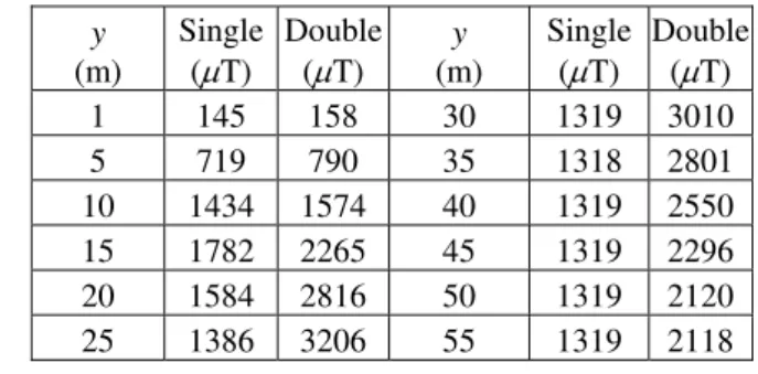
The FEM-based simulation conducted in this paper is coded with MATLAB programming for calculation of magnetic field dispersion. To utilize a graphical feature of MATLAB, thecontour of magnetic field distribution through the cross-sectional area of the working domain for the single- and double-circuit transmission systems are presented in Fig. 5 and Fig. 6, respectively.

Fig. 5 Magnetic field distribution (μT) for the single-circuit case

Fig. 6 Magnetic field distribution (μT) for the double-circuit case

The illustration of magnetic field contour for both single- and double-circuit systems is given by a working area of the 70×55 m2 rectangle as shown in Fig. 3 and Fig. 4, respectively. The magnetic field distributions simulatedare determined by balanced carrying currents in the phase conductors. Magnetic field distribution of the double-circuit case is higher than that of the single-circuit case. To describe possible effects of magnetic field strength on human or other living things underneath the power line, the line of

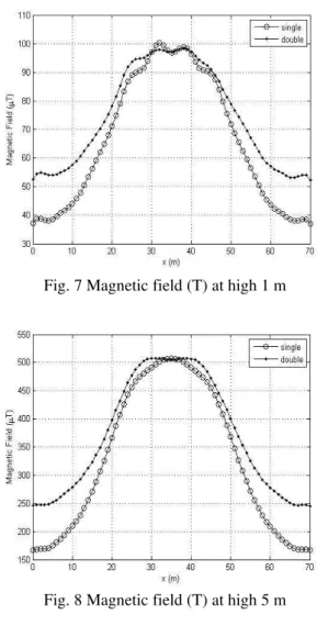
calculation, 1.0 m above the ground (y = 1 m) is defined. The comparative result of magnetic field for both single- and double-circuit cases is shown in Fig. 7. It notices that each graph has two peaks near the center position.

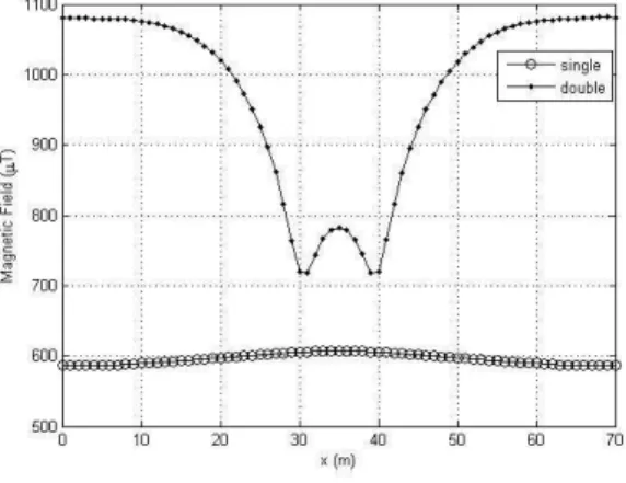
Table I showed the result of comparison in magnetic field distribution through distance x when consider single and double circuit transmission line that is over from the ground level 1 m that people pass by. An average of magnetic field through distance x of single and double circuit when consider the height of transmission line at midspan and consider at maximum load current are 65.88 μT and 74.18 μT, respectively, which is less than magnetic field level that hazard to human. It is regulated by International Commission of Non Ionizing Radiation Protection [16], which the level of magnetic field safe to human for general public up to 24 hours/day must not greater than 100 μT and for occupation whole working day must not over 500 μT. Fig. 8 - Fig .18 are graphs representing the magnetic fields of both single and double circuit cases at a position of 5, 10, 15, 20, 25, 30, 35, 40, 45, 50 and 55 m above ground level, respectively. Table II showed comparative results among average magnetic field for all the cases. It is considered that at the same height, the double circuit distributes more intensive magnetic field than the single circuit does due to twice of the conductor number.

Fig. 7 Magnetic field (T) at high 1 m

(5)

(6)

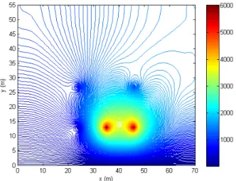
B. Fault Conditions

The contour of magnetic field distribution through the cross-sectional area of the working domain for the single-circuit transmission systems for four faulted conditions (single line-to-ground faults, double line-to-ground faults, line-to-line faults and balanced three-phase faults) are presented in Fig. 19 - Fig. 22, respectively. The double-circuit transmission systems for the four faulted cases are presented in Fig. 23 - Fig. 26, respectively.

Fig. 19 Magnetic field distribution (μT) for the single-circuit case of the single line-to-ground faults

Table I

Comparing of magnetic field dispersion at high1 m x

(m)

Single (μT)

Double (μT)

x (m)

Single (μT)

Double (μT) 1 37.11 52.54 36 97.17 97.41 2 38.67 54.57 37 98.28 98.04 3 38.74 54.84 38 98.87 98.36 4 38.34 54.42 39 98.28 98.10 5 38.18 54.00 40 96.38 97.20 6 38.60 53.96 41 93.77 95.79 7 39.56 54.34 42 91.59 94.35 8 40.72 54.98 43 90.74 93.35 9 41.74 55.69 44 90.40 92.39 10 42.77 56.52 45 89.49 91.02 11 44.06 57.59 46 87.40 89.13 12 45.76 58.94 47 84.04 86.75 13 47.95 60.60 48 79.83 84.04 14 50.60 62.52 49 75.54 81.33 15 53.46 64.49 50 71.87 78.94 16 56.25 66.34 51 68.64 76.71 17 59.04 68.23 52 65.57 74.44 18 61.92 70.33 53 62.54 72.07 19 64.88 72.69 54 59.54 69.63 20 67.91 75.33 55 56.58 67.17 21 71.14 78.25 56 53.59 64.72 22 74.83 81.59 57 50.54 62.29 23 79.13 85.38 58 47.72 60.11 24 83.39 89.00 59 45.41 58.36 25 86.83 91.85 60 43.66 57.04 26 89.02 93.68 61 42.39 56.10 27 90.05 94.54 62 41.44 55.37 28 90.52 94.75 63 40.51 54.64 29 91.50 94.99 64 39.40 53.81 30 93.94 95.91 65 38.46 53.18 31 96.97 97.02 66 38.03 53.07 32 99.43 97.78 67 38.18 53.51 33 100.33 98.00 68 38.57 54.12 34 99.47 97.74 69 38.54 54.11 35 97.81 97.24 70 37.03 52.37

Average 65.88 74.18

Table II

Comparing of average of magnetic field at each height y

(m)

Single (μT)

Double (μT)

y (m)

Single (μT)

Double (μT)

1 66 74 30 596 1288

5 327 371 35 596 1299

10 652 740 40 596 1182

15 810 1016 45 596 1061

20 719 1157 50 596 978

(7)

Fig. 20 Magnetic field distribution (μT) for the single-circuit caseof the double line-to-ground faults

Fig. 21 Magnetic field distribution (μT) for the single-circuit case of the line-to-line faults

Fig. 22 Magnetic field distribution (μT) for the single-circuit case of the balanced three-phase faults

Fig. 23 Magnetic field distribution (μT) for the double-circuit case of the single line-to-ground faults

Fig. 24 Magnetic field distribution (μT) for the double-circuit case of the double line-to-ground faults

Fig. 25 Magnetic field distribution (μT) for the double-circuit case of the line-to-line faults

(8)

Fig. 26 Magnetic field distribution (μT) for the double-circuit case of thebalanced three-phase faults From Fig. 19 - Fig. 26,magnetic field contour of the faulted cases for both single- and double-circuit systems are presented.Table III – VI show the average of magnetic fields for both single- and double-circuit systems at each height when the single line-to-ground faults, double line-to-ground faults, line-to-line faults and balanced three-phase faults are occurred, respectively. As can be seen, the magnetic field intensity caused by the faulted cases is remarkably higher than that of the normal conditions. However, due to the reliable operation of protective devices in electric power systems this could not harm human or other living things underneath the EHV power lines.

Table III

Average of magnetic field at each height of the single line-to-ground faults

y (m)

Single (μT)

Double (μT)

y (m)

Single (μT)

Double (μT)

1 119 142 30 1091 2086

5 591 715 35 1091 2463

10 1177 1424 40 1091 2241

15 1462 1801 45 1091 2001

20 1307 1699 50 1091 1835

25 1145 1691 55 1091 1834

Table IV

Average of magnetic field at each height of the double line-to-ground faults

y (m)

Single (μT)

Double (μT)

y (m)

Single (μT)

Double (μT)

1 147 160 30 1334 3036

5 727 799 35 1333 2828

10 1450 1593 40 1334 2575

15 1802 2289 45 1334 2319

20 1603 2842 50 1334 2141

25 1402 3233 55 1335 2139

Table V

Average of magnetic field at each height of the line-to-line faults

y (m)

Single (μT)

Double (μT)

y (m)

Single (μT)

Double (μT)

1 145 158 30 1319 3010

5 719 790 35 1318 2801

10 1434 1574 40 1319 2550

15 1782 2265 45 1319 2296

20 1584 2816 50 1319 2120

25 1386 3206 55 1319 2118

Table VI

Average of magnetic field at each height of thebalanced three-phase faults

y (m)

Single (μT)

Double (μT)

y (m)

Single (μT)

Double (μT)

1 213 240 30 1949 4159

5 1060 1199 35 1948 4196

10 2113 2390 40 1949 3819

15 2626 3282 45 1949 3428

20 2339 3736 50 1949 3158

25 2047 4098 55 1950 3155

V. CONCLUSION

This paper has studied the magnetic field distribution surrounding EHV transmission line in both normal loadings and faulted conditions in which the single line-to-ground faults, double line-to-ground faults, line-to-line faults and balanced three-phase faults were situated. Single- and double-circuit, 500-kV transmission lines of Electricity Generating Authority of Thailand (EGAT), which is recently the highest voltage level in Thailand, are investigated. The computer simulation is performed by using finite element methods instructed in MATLAB programming codes. The results of the normal loading caserevealed that the magnetic fields from both single- and double-circuit, 500-kV transmission lines at a level of 1m above the ground that are assumed to be the level of human working, do not excess the maximum allowance when compiled with the ICNIRP standard. Additionally, the results also showed that the magnetic intensity of the double circuit cases is normally stronger than those of the single circuits.

REFERENCES

[1] Y. Du, T.C. Cheng and A.S. Farag, “Principles of Power-Frequency Magnetic Field Shielding with Flat Sheets in a Source of Long Conductors,” IEEE Transactions on Electromagnetic Compatibility, Vol. 38, No. 3, pp.450-459, 1996.

[2] A.R. Memari and W. Janischewskyj, “Mitigation of Magnetic Field near Power Lines,” IEEE Transactions on Power Delivery, Vol. 11, No. 3, pp.1577-1586, 1996.

[3] K. Wassef, V.V. Varadan and V.K. Varadan, “Magnetic Field Shielding Concepts for Power Transmission Lines,” IEEE

Transactions on Magnetics, Vol. 34, No. 3, pp.649-654, 1998.

(9)

[5] L. Li and G. Yougang, “Analysis of Magnetic Field Environment near High Voltage Transmission Lines,” Proceedings of the International

Conferences on Communication Technology, pp.S26-05-1 - S26-05-5,

1998.

[6] M.V.K. Chari and S.J. Salon, Numerical Methods in Electromagnetism, Academic Press, USA, 2000.

[7] M. Weiner, Electromagnetic Analysis Using Transmission Line

Variables, World Scientific Publishing, Singapore, 2001.

[8] C. Christopoulos, The Transmission-Line Modeling Method: TLM, IEEE Press, USA, 1995.

[9] P. Pao-la-or, T. Kulworawanichpong, S. Sujitjorn and S. Peaiyoung, “Distributions of Flux and Electromagnetic Force in Induction Motors: A Finite Element Approach,” WSEAS Transactions on Systems, Vol. 5, No. 3, pp.617-624, 2006.

[10] P. Pin-anong, The Electromagnetic Field Effects Analysis which Interfere to Environment near the Overhead Transmission Lines and

Case Study of Effects Reduction, M. Eng. Thesis, King Mongkut’s

Institute of Technology Ladkrabang, Bangkok, Thailand, 2002. [11] T.W. Preston, A.B.J. Reece and P.S. Sangha, “Induction Motor

Analysis by Time-Stepping Techniques,” IEEE Transactions on

Magnetics, Vol. 24, No. 1, pp.471-474, 1988.

[12] B.T. Kim, B.I. Kwon and S.C. Park, “Reduction of Electromagnetic Force Harmonics in Asynchronous Traction Motor by Adapting the Rotor Slot Number,” IEEE Transactions on Magnetics, Vol. 35, No. 5, pp.3742-3744, 1999.

[13] G.B. Iyyuni and S.A. Sebo, “Study of Transmission Line Magnetic Fields,” Proceedings of the Twenty-Second Annual North American,

IEEE Power Symposium, pp.222-231, 1990.

[14] M.E. El-Hawary, Electrical Energy Systems, CRC Press, USA, 2000. [15] Jr.W.H. Hayt and J.A. Buck, Engineering Electromagnetics (7th

edition), McGraw-Hill, Singapore, 2006.

[16] International Commission of Non Ionizing Radiation Protection (ICNIRP), “Guidelines for Limiting Exposure to Time-Varying Electric, Magnetic and Electromagnetic Fields (up to 300 GHz),”

Health Phys., Vol. 74, No. 4, pp.494-522, 1998.