Symmetries as a guide to regularization ambiguities: Standard and
Beyond Standard Model examples
Adriano Lana Cherchiglia
Orientador: Prof. Dr. Marcos Donizeti R. Sampaio
Departamento de F´ısica
Universidade Federal de Minas Gerais
Tese apresentada `a UNIVERSIDADE FEDERAL DE MINAS
GERAIS, como requisito
para obten¸c˜ao do grau de
Doutor em F´ısica.
Dedico esta tese `aquela que sempre me faz ir mais longe do que
pensava ser capaz. Obrigado por sempre me apoiar,
Acknowledgements
Agrade¸co a Deus, por tudo.
Agrade¸co a minha noiva Marceli de Aquino, por estar sempre presente ao meu lado, tanto nos momentos bons mas especialmente nos dif´ıceis. Obrigado por toda a sua paciˆencia, carinho, amor e dedica¸c˜ao, por sempre me incentivar a ser uma pessoa melhor, e, sobretudo, por me fazer feliz, a cada dia.
Agrade¸co a meus pais Antonio Carlos e Beatriz, por toda a educa¸c˜ao, forma¸c˜ao e amor que me deram, que me permitiram ser quem sou e chegar at´e aqui.
Agrade¸co a minha irm˜a Let´ıcia, pelo seu companheirismo em todas as horas.
Agrade¸co ao Marcos, por todo o apoio que me tem dado durante todos esses anos. Por tudo o que aprendi, pelas oportunidades que me ofereceu, e, sobretudo, por ter me mostrado o que ´e ser um verdadeiro profissional. Por ter sido muito mais do que orientador, mas um verdadeiro amigo.
Agrade¸co `a Carolina, por tudo o que me ensinou, tanto na F´ısica, mas tamb´em como pessoa. Sou muito grato por ter tido a oportunidade de estar ao lado de algu´em t˜ao ´unico como ela durante todos esses anos.
Agrada¸co ao Jean, por todos os momentos que passamos juntos, fazendo contas ou conversando da vida. Foi um prazer poder contar com vocˆe, compa˜nero!
Agrade¸co ao Cabral, Gustavo, Helv´ecio, por estarem sempre dispon´ıveis e dispostos.
Agrade¸co ao Prof. Perez-Victoria por ter me recebido no seu grupo de maneira t˜ao acolhedora e por todas as discuss˜oes frut´ıferas que tivemos juntos. Por todas as oportunidades que ele me proporcionou e que foram determinantes para a conclus˜ao dessa tese.
Agrade¸co a todos os amigos que fiz em Granada e por tudo o que puder aprender com eles, a como ser um melhor f´ısico e ser humano.
Agrade¸co ao pessoal do grupo de TQC, Alexandre, Joilson, Yuri, Arthur, Helder por todos os momentos em que pudemos aprender uns com os outros.
Agrade¸co a toda a minha fam´ılia que sempre me apoiou em fazer aquilo de que gostava e sempre esteve do meu lado sempre que precisei. Agrade¸co em especial aos meus tios Luiz e Mariangela, por todo apoio em todas as horas.
Agrade¸co a todos os meus tios, tias, primos e av´os, pelos momentos que pudemos conviver juntos e disfrutar da companhia um dos outros.
Agrade¸co a Shirley e toda a equipe da biblioteca, assim como toda a equipe da secretaria, por serem sempre atenciosos e prestativos.
Abstract
This thesis is about regularization of ultraviolet divergences appear-ing in the perturbative expansion of quantum field theories (QFT’s). We present a general view of the ambiguities that may arise in the regularization program and develop a systematic approach to extract them from a general Feynman amplitude. We show that they are inti-mately related with the breaking of the symmetries of the underlying quantum field theory. We also show they are related to the viola-tion of momentum routing invariance (MRI) of Feynman diagrams, allowing us to regard MRI as a symmetry to be preserved in the per-turbative expansion of QFT’s. We apply our formalism to a variety of theories and examples such as: the Higgs decay to two photons, the photon-photon scattering, and N=1 supersymmetric electrody-namics. In all cases we verify that regularization ambiguities can be consistently extracted being related to the breaking of the symmetries of the underlying QFT. We also study the role played by quadratic divergences on a variety of examples showing its connection (or not) to the ambiguities aforementioned.
Declaration
This thesis is the result of research carried out between March 2011 and July 2014. The work presented in this thesis has not been sub-mitted in fulfillment of any other degree or professional qualification.
Contents
Contents vi
1 Introduction 1
2 Technicalities: the regularization program and how to deal with
regularization ambiguities 6
2.1 The rules of implicit regularization . . . 8
3 Momentum Routing Invariance in Feynman Diagrams and
Quan-tum Symmetry Breakings 12
3.1 Momentum Routing Invariance and Surface Terms atn-loop order 14 3.2 Momentum Routing Invariance and QED Ward Identities . . . 19 3.3 Momentum Routing Invariance in the context of scalar field theories 24
4 (Un)determined finite regularization dependent quantum correc-tions: the Higgs decay into two photons and the two photon
scattering examples 27
4.1 A general view of regularization dependent integrals . . . 29 4.2 Higgs decay into two photons . . . 33 4.3 Two photon scattering . . . 37
5 Guises and Disguises of Quadratic Divergences 40
5.1 Basic divergent integrals, regularization ambiguities and parametriza-tions . . . 45 5.2 Example: Cancelation of Quadratic Divergences and
CONTENTS
5.3 Higgs decay to two photons . . . 56 5.4 Quadratic Divergences and Effective Theories: Nambu-Jona-Lasinio
model . . . 61 5.5 Hierarchy problem . . . 64
6 Controversy on the background field method: massless N = 1
supersymmetric electrodynamics as an example 71
6.1 Massless N = 1 supersymmetric electrodynamics . . . 73 6.2 Discussion of the results and perspectives . . . 88
7 Conclusion and perspectives 91
Appendix A 93
Appendix B 94
Chapter 1
Introduction
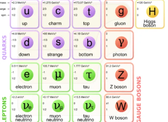
The Standard Model of Elementary Particles (SM) is one of the major achieve-ments of the human mind. Relying on aesthetic and simple concepts like sym-metries, physicists developed a consistent theory capable of describing three of the four fundamental interactions found in Nature as well as its particle content. Recently, one of the lacking fundamental blocks of the theory (the Higgs boson) was finally found corroborating this journey toward answering a question that mankind has been asking since the Greeks: what are we and Nature itself made of? At present, the answer could be summarized in the table below [1]:
Figure 1.1: Particle content of the Standard Model
1. Introduction
L=−1
4FµνF
µν +iψ /¯Dψ+ ¯ψ
iyijψjφ+ h.c. +|Dµφ|2−V(φ). (1.1)
From a theoretical point of view, once one has the Lagrangian of a theory, all the techniques and strategies systematized in the subject of Quantum Field Theory can be promptly applied. Pragmatically, one has the following
L→Feynman rules→Feynman diagrams →compute S-matrix elements
In other words, by using (1.1) one is, in principle, capable of predicting any elementary particle process.
This situation is particular interesting when one intends to obtain the mag-netic moment of the muon, for instance. The first point to be emphasized is that there is a quantum mechanical anomaly, which means that the value of the mag-netic moment of the muon, after quantization of the classical theory, is different from the one predicted by the classical theory. In the particular example of the muon one has
µ= e~ 2mµ
(1 +aµ), (1.2)
where aµ is the anomalous term. At present, this is one of the most accurate
measured quantities in Physics whose value we quote below [2]
aexp
µ = 116 592 089(54)stat(33)syst(63)tot×10−11 (±0.54ppm). (1.3)
Such accurate result motivates, from the theoretical side, an equally accurate prediction. The state of art, at present, takes into account QED contributions up to five loops, electroweak (EW) contributions up to two loops and lead with hadronic vacuum polarization loops (HVP) as well as hadronic light-by-light scat-tering (HLbyL). A recent evaluation is given in [3]
aSM
µ = 116 591 802(42)HVP(26)HLbyL(2)QED+EW(49)tot×10−11 (±0.42ppm). (1.4)
1. Introduction
to obtain such precise theoretical result one has to resort to multiloop calcula-tions, which motivates the development of techniques to deal properly with such involved calculation. To properly discuss the subject of multiloop computations, one has to take a step backward and discuss the regularization/renormalization program itself.
As is well known, in Quantum Field Theory (QFT) one in general has to deal with infinities. They may appear in any calculation even at first order in perturbation theory, which urged a method to make some sense of them.1.It is in this context that the renormalization program appeared which allows one to group all the infinities in the bare parameters of the theory we are dealing with. If this procedure is always possible, one says that the theory is renormalizable. In the past, renormalizability was a feature that all good theory should share, along with Lorentz invariance, for instance. Nowadays, the perspective has shifted a little, especially after the introduction of the concept of effective field theories (and consistent techniques to deal with them). In any case, even if the requirement of renormalizability is not as strong as it was in the past (it was one of the criterion used in the construction of the Standard Model, for instance), one is not excused away of the task of dealing with infinities which requires the introduction of some regularization method. At present, we have a variety of techniques, all with their advantages and disadvantages. However, all of them share one specific behavior: by making sense of the divergent integral (in other words, evaluating it to some value) one is implicit preserving (or not) some symmetries of the theory at hand. For instance, Dimensional Regularization is known to preserve automatically gauge invariance while introducing a cutoff is known to break such symmetry. In any case, it would be advantageous if, instead of automatically preserving (or not) a symmetry, one had the possibly to identify the ambiguities introduced by the regularization procedure. Therefore, the ambiguities would be fixed by imposing the symmetries (or experimental input) of the model. This feature is particular interesting in the case of quantum mechanical anomalies, for instance, in the ABJ chiral anomaly that we are going to discuss in detail
1It should be emphasized that this behavior is not a characteristic of the method of
1. Introduction
in chapter 3. As we will comment there, the classical model posses a gauge and chiral symmetry, one of which is broken upon quantization. In our point of view, both symmetries are equally important and there is no reason a priori to decide which one should be preserved by the regularization method, this choice should be left to experiments.
This is the point of view we are going to develop and systematize through out this thesis. We intend to present a consistent way to deal with regularization ambiguities, more specifically, how to identify and express them even in multiloop calculations. Once identified, we proceed to fix them by imposing the symmetries of theory which can (or not) be always enough to produce a definite answer. In the examples we are going to present in this thesis, which encompass Standard and Beyond Standard Model processes, we will always obtain a definite answer, the only exception being the ABJ chiral anomaly we had already commented about. However, this may not be always the case as discussed in [4] where an ambiguous result is obtained.
Overview of the thesis
This thesis will be presented in cumulative form. Each subsequent chapter will contain the results of a work already published or submitted.
• Chapter 2mostly contains the technical part of the thesis. We present the Implicit Regularization technique in its most general form, applicable to multiloop Feynman diagrams. We also present how regularization depen-dent terms (called surface terms) can be idepen-dentified and extracted from a general amplitude.
1. Introduction
study a scalar theory and shows that demanding MRI is crucial in order to obtain the two-loop universal coefficients of the beta function.
• In chapter4we apply the discussion carried out in the two previous chapters in two specific examples: the Higgs decay to two photons and the two photon scattering. In both cases we give an answer for a debate in the literature about the regularization dependent character of finite quantum corrections. We show how the many results found in the literature can be explained in our formalism and discuss, once again, the interplay between MRI and gauge invariance.
• Chapter 5contains a extended discussion about quadratic divergences. We present how they can be properly treated in our formalism by introducing a general parametrization for divergences. Therefore, we can add a cutoff to our theory but not losing control of regularization dependent terms ex-pressed by surface terms. We revisit some problems by this new perspective such as 1-loop renormalization QCD and the Higgs decay to two photons presented in the previous chapter. We also briefly discuss the importance of quadratic divergences for effective models of QCD (Nambu-Jona-Lasinio model in particular). Finally we present how the hierarchy problem can be translated in our formalism, showing that it is related to ambiguities coming from quadratic divergences.
Chapter 2
Technicalities: the regularization
program and how to deal with
regularization ambiguities
Introduction
complying with locality, Lorentz invariance, unitarity and causality.
To calculate S-matrix elements in a symmetry preserving fashion in a quan-tum field theoretical model sensitive to dimensional continuation on the space-time, the problem is more subtle. The construction of an invariant regularization framework is aesthetically more appealing but this is not the main motivation. Although in one hand imposing constraint equations derived from Ward identi-ties order by order in perturbation theory obliterates the need of an invariant regularization, on the other hand it renders the calculation more involved from the calculational viewpoint. Besides, if quantum symmetry breakings occur in perturbation theory, an invariant scheme is essential to judge it as physical or spurious. Supersymmetric gauge theories are conspicuous examples of models in which regularization and renormalization play a fundamental role especially as new accurate experimental evidence, viz. electroweak precision observables [14,15,16,17], demands consistent theoretical calculations higher than one loop order to understand physics beyond the Standard Model.
can be treated within the same strategy after space time and internal algebra are performed.
2.1
The rules of implicit regularization
We restrict ourselves to massless theories and power counting infrared safe inte-grals. The first restriction is justified because, as we showed in [34], to implement a mass independent renormalization scheme in IReg we need only the massless basic divergent integrals that we present below. When infrared divergences do appear, a dual version of IReg operating in coordinate space displays infrared divergences as basic divergent integrals as well, in a way that infrared and ultra-violet degrees of freedom are clearly distinguished [35, 36,37].
Given the amplitude of an-loop Feynman graph withLexternal legs, the basic strategy of IReg is to free all divergences of external momenta and express them in terms of basic divergent integrals in one loop momentum only. To achieve this purpose, we need to perform (n−1) integrations, but the order in which they are performed is not clear a priori. In [34] we presented a systematic way to choose the order of integration which, as a byproduct, displays the counterterms to be subtracted by Bogoliubov’s recursion formula. Considering that we made this choice, we can redefine the internal momenta in such a way that the integral in
kl is the l-th we are going to deal with and it is typically of the form
Iν1...νm=
Z
kl
Aν1...νm(k
l, qi)
Q
i[(kl−qi)2−µ2]
lnl−1
−k 2
l −µ2
λ2
, (2.1)
where l = 1· · ·n. In the above equation, qi is an element (or combination of
elements) of the set {p1, . . . , pL, kl+1, . . . , kn},
R
kl ≡
R
ddk
l/(2π)d and µ2 is an
infrared regulator.
Since the original integral is infrared safe, the limit µ2 → 0 is well-defined
(renor-malization group scale). It appears at one loop level and survives to higher orders through a regularization independent mathematical identity (eq. 2.11) as we show in the end of this section. The function Aν1...νm(k
l, qi) may contain constants and
all possible combinations of kl and qi compatible with the Lorentz structure.
Care must be exercised when it contains a term like (kl−qi)2. In this case, we
must cancel it against one of the denominators because, as we are dealing with divergent integrals, symmetric integration is a forbidden operation [23], [39]. In chapter 4we will study a particular example in which this prescription is vital to obtain a well defined, gauge invariant result.
Now, we apply the rules of IReg. Assuming that a regulator Λ is implicit in the integral, we can use the following mathematical identity in the denominators:
1 (kl−qi)2−µ2
=
n(ikl)−1
X
j=0
(−1)j(q2
i −2qi·kl)j
(k2
l −µ2)j+1
+ (−1)
n(ikl)(q2
i −2qi·kl)n
(kl)
i
(k2
l −µ2)n
(kl)
i [(kl−qi)2−µ2]
. (2.2)
The values ofn(kl)
i are chosen such that all divergent integrals have a
denom-inator free of qi.
After the use of (2.2), the divergent integrals can be casted as a combination of
Ilog(l)(µ2)≡
Λ
Z
kl
1 (k2
l −µ2)d/2
lnl−1
−k 2
l −µ2
λ2
, (2.3)
I(l)ν1···νr
log (µ2)≡
Λ
Z
kl
kν1
l · · ·klνr
(k2
l −µ2)β
lnl−1
−k 2
l −µ2
λ2
or
Iquad(l) (µ2)≡
Λ
Z
kl
1 (k2
l −µ2)
d−2 2
lnl−1
−k 2
l −µ2
λ2
, (2.5)
I(l)ν1···νr+2
quad (µ
2) ≡
Λ
Z
kl
kν1
l · · ·k νr+2
l
(k2
l −µ2)β
lnl−1
−k 2
l −µ2
λ2
, (2.6)
where r = 2β −d. It is important to note that only these type of divergences appear because linear BDI’s always vanish1. Although we have already reduced the divergences to basic divergent integrals free of external momenta, we can show that the integrals defined above are related. For example, in a case with two Lorentz indices we have
Ilog(l)µν(µ2) =
l X j=1 2 d j
(l−1)! (l−j)!
gµν
2 I
(l−j+1)
log (µ2)−
1 2Υ
(l)µν
0
, (2.7)
where Υ(0l)µν ≡R
k ∂ ∂kµ
h
kν
(k2−µ2)d/2 ln
l−j
−k2λ−2µ2 i
, and
Iquad(l)µν(µ2) =
l
X
j=1
2
d−2
j
(l−1)! (l−j)!
gµν
2 I
(l−j+1)
quad (µ2)−
1 2Υ
(l)µν
2
, (2.8)
where Υ(2l)µν ≡
R k ∂ ∂kµ kν
(k2−µ2)d−22 ln
l−j
−k2λ−2µ2
.
In the previous equations, Υ(0l)µν, and Υ(2l)µν are (arbitrary) regularization depen-dent surface terms. In a more general case they are given by
Υ(l)ν1···νj
i ≡
Z
ddk
(2π)d
∂ ∂kν1
kν2· · ·kνj (k2−µ2)d+j−22−i ln
l−1
"
− (k
2 −µ2) λ2
#
. (2.9)
1We are considering only theories with even dimensions. For odd dimensions, an equivalent
An equivalent definition in terms of Lorentz scalar objects Γ(il,j) is
g{ν1···νj}Γ(l,j)
i ≡Υ
(l)ν1···νj
i , (2.10)
where g{ν1···νj} ≡gν1ν2· · ·gνj−1νj+ symmetric combinations.
Finally the divergences can be written in terms of (2.3) and (2.5). However from (2.3) we see that this integral is ultraviolet and infrared divergent asµ2 →0.
In order to separate these divergences and define a genuine ultraviolet divergent object we use the regularization independent relation
Ilog(l)(µ2) = Ilog(l)(λ2)−bd
l ln
l
µ2 λ2
+bd A
X
k=1
A k
Xl−1
j=1
(−1)k
kj
(l−1)! (l−j)!ln
l−j
µ2 λ2
,
(2.11)
where λ2 6= 0, A≡ (d−2)
2 , bd≡
i
(4π)d/2
(−1)d/2
Γ(d/2). (2.12)
For infrared safe models the infrared divergence must cancel in the amplitude as a whole. This in fact occurs because, as we use identity (2.2), the finite part of the amplitude will also have a logarithmical dependence in µ2 which exactly
Chapter 3
Momentum Routing Invariance
in Feynman Diagrams and
Quantum Symmetry Breakings
Introduction
In the 1972 seminal paper by ’t Hooft and Veltman [12] on dimensional regular-ization (DReg), they emphasized that besides respecting unitarity and causality, DReg also allowed for shifts in integration variables (loop momenta) of Feynman amplitudes. When no quantum symmetry breakings occurred, Ward identities were automatically satisfied crowning DReg as the ideal framework to handle ul-traviolet divergences in perturbation theory of gauge theories. Indeed it is well known that the possibility of shifts in the integration variable is an important ingredient for diagrammatic proofs of gauge invariance in quantum electrodynam-ics.
dimen-sion but not in dimendimen-sionally continued space-times. Such ambiguities were used by the authors to warrant the validity of Ward-Slavnov-Taylor identities in some model calculations at one-loop level. In other words, this approach, called Pre-regularization, used integration variable ambiguities in four dimensional loop in-tegrals to parametrize the divergent amplitudes in a way that Ward identities were preserved by a suitable choice of the routing labels in the loop of a dia-gram. Anomalies, such as the well known Adler-Bardeen-Bell-Jackiw triangle chiral anomaly, appear in this approach when the ambiguities proved themselves insufficient to preserve the full set of symmetry identities valid at classical level. Of course Dimensional Reduction (DRed) is the most popular tool to perform Feynman diagram calculations in supersymmetric gauge theories and other di-mension specific models which require modifications in gauge symmetry preserv-ing dimensional regularization. Generalizations of DRed which ensure invariance to two-loop order in models of phenomenological importance have been done [41], but it is still unknown to what extent it preserves supersymmetry. An invariant
regularization framework , which avoids the task of computing symmetry restor-ing counterterms order by order in perturbation theory for dimensional sensitive theories is hitherto unknown. In other words, the construction of an invariant regularization scheme to compute with supersymmetric gauge theories is justified on practical and theoretical grounds.
3.1
Momentum Routing Invariance and Surface
Terms at
n-loop order
In this section we study the conditions which guarantee MRI to an arbitrary multi-loop Feynman diagram. We find that the only condition needed to preserve such symmetry is to set surface terms to zero.
As it is well known, if f(k) is an arbitrary function, then
f(k+a) = f(k) +aσ
∂ ∂kσ
f(k) + aσaρ 2!
∂ ∂kσkρ
f(k) +· · ·
=exp
aσ
∂ ∂kσ
f(k). (3.1)
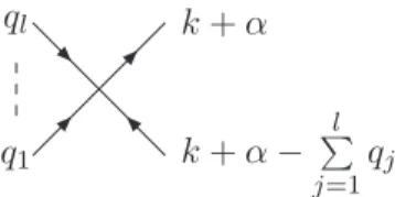
We now consider an arbitrary graph at one-loop order. Settingkas its internal momentum, and qi as the external momenta we will have in general, for any
theory, a vertex of the type depicted in figure 3.1.
q1
ql k+α
k+α− Pl
j=1
qj
Figure 3.1: Generic vertex with arbitrary momentum routing α.
Therefore, the amplitude of this graph can be expressed as
A ≡
Z
ddk
(2π)df(k+α, qi), (3.2)
where for simplicity we consider a scalar amplitude, although the generalization for amplitudes with an arbitrary number of Lorentz indices is straightforward. We now present the cornerstone of our argument: if we have momentum routing invariance then
Z
ddk
(2π)df(k+α, qi)−
Z
ddk
must be satisfied for arbitrary α and β. Using identity (3.1) it reduces to
Z
ddk
(2π)d
exp
ασ
∂ ∂kσ
f(k, qi)−
Z
ddk
(2π)d
exp
βσ
∂ ∂kσ
f(k, qi) = 0. (3.4)
For simplicity, we will consider f(k, qi) as a linear divergent integral. Therefore,
by applying a regularization (for example, IReg) one obtains
Z ddk
(2π)d
flin(k, qi) +flog(k, qi) +ff in(k, qi) +ασ
∂ ∂kσ
flin(k, qi)
−
Z
ddk
(2π)d
flin(k, qi) +flog(k, qi) +ff in(k, qi) +βσ
∂ ∂kσ
flin(k, qi)
= 0,
(ασ −βσ)
Z
ddk
(2π)d
∂ ∂kσ
flin(k, qi) = 0 (3.5)
since ifB ≡R ddk
(2π)d
∂f(k)
∂kσ andf(k) is finite or logarithmic divergent, then by Gauss’ theorem B is null.
This would be the condition to implement MRI for linear divergent integrals. To proceed and make explicit the connection with surface terms, we must analyze further the function f(k, qi). After space-time and internal group algebra are
performed, f(k, qi) is given by
f(k, qi) =
g(k, qi) L
Q
j=1
[(k+lj(qi))2−µ2]
(3.6)
where g(k, qi) and lj(qi) are polynomials in the momenta and µ2 is an infrared
regulator. The divergence of such integral is controlled by the dimension of the theory (d), the number of internal lines (L), and the degree inkof the polynomial
g(k, qi) which we define as m.
Evidently, ifd+m−2L≤0 condition (3.4) is automatically satisfied as loga-rithmic divergent graphs are always momentum routing invariant. We proceed to linear divergent integrals which, after using the identity of IReg in all propagators one time, furnishes:
In view of the comments above only the first term is of interest to us. Its general form is given by
Z
ddk
(2π)dflin(k, qi) =
Z
ddk
(2π)d
Q
i(k·qi)bi
Q
k(qi·qk)cik
[k2−µ2]L , (3.8)
where d+s−2L= 1, s ≡Pibi, and we canceled powers ofk2 in the numerator
against propagators. This cancellation must always be performed because, as we are dealing with divergent integrals, symmetric integration is forbidden [23], [39].
In this case, condition (3.4) is satisfied only if
(ασ−βσ)
Z
ddk
(2π)d
∂ ∂kσ
flin(k, qi) = (ασ−βσ)hν1···νs(qi)
Z
ddk
(2π)d
∂ ∂kσ
kν1· · ·kνs [k2−µ2]L = 0.
(3.9) Since α, β are arbitrary, and hν1···νs(qi) is a polynomial in qi, we notice that the condition above is equivalent to the statement (see equation (2.9))
Υ(1)σν1···νs
0 = 0. (3.10)
In other words, momentum routing invariance is guaranteed for linearly di-vergent graphs only if surface terms are systematically set to zero. We consider now quadratically divergent integrals which, after using identity (2.2) in all prop-agators two times, gives:
f(k, qi) =fquad(k, qi) +flin(k, qi) +flog(k, qi) +ff in(k, qi). (3.11)
Since linear, logarithmical and finite cases were already analysed, we only need to deal with the first term which is
Z
ddk
(2π)dfquad(k, qi) =
Z
ddk
(2π)d
Q
i(k·qi)bi
Q
k(qi·qk)cik
[k2−µ2]L , (3.12)
Now, condition (3.4) is satisfied only if
(ασ−βσ)
Z
ddk
(2π)d
∂ ∂kσ
fquad(k, qi) = (ασ−βσ)hν1···νs(qi)
Z
ddk
(2π)d
∂ ∂kσ
kν1· · ·kνs [k2−µ2]L = 0,
(3.13) and
(ασ−βσ)(αρ−βρ)
Z
ddk
(2π)d
∂2 ∂kσ∂kρ
fquad(k, qi) = (ασ−βσ)(αρ−βρ)hν1···νs(qi)×
×
"
gν1ρ Z
ddk
(2π)d
∂ ∂kσ
kν2· · ·kνs [k2 −µ2]L +
s−1
X
j=2 gνjρ
Z
ddk
(2π)d
∂ ∂kσ
kν1· · ·kνj−1kνj+1· · ·kνs [k2−µ2]L +
+gνsρ
Z ddk
(2π)d
∂ ∂kσ
kν1· · ·kνs−1
[k2−µ2]L −2L
Z ddk
(2π)d
∂ ∂kσ
kν1· · ·kνskρ [k2−µ2]L+1
#
= 0. (3.14)
The relations above are equivalent to the statements
Υ(1)1 σν1···νs = 0,
Υ(1)σν2···νs
0 = 0, Υ
(1)σν1···νj−1νj+1···νs
0 = 0, Υ
(1)σν1···νs−1
0 = 0 and Υ
(1)σν1···νsρ
0 = 0.
(3.15)
Therefore, we conclude that momentum routing invariance is guaranteed for quadratically divergent graphs only if surface terms are systematically set to zero. This result can be generalized to graphs with any kind of divergence proving that momentum routing invariance is verified only if we set all surface terms to zero. Although our results are restricted to one-loop order in perturbation theory, a general proof for arbitrary Feynman diagrams can also be developed. We present in the following the demonstration for two-loop graphs and state how it can be further generalized to an arbitrary number of loops.
Assume that the amplitude of a two-loop process is given by,
A(2) ≡
Z
ddk1
(2π)d
ddk2
(2π)df(k1+α1, k2+α2, qi), (3.16)
momenta qi. Once again, momentum routing invariance is guaranteed by the
condition
Z ddk
1
(2π)d
ddk
2
(2π)d
" 2 Y
j=1
exp ασj
j
∂ ∂kσj
j ! − 2 Y j=1
exp βσj
j
∂ ∂kσj
j
!#
f(k1, k2, qi) = 0.
(3.17) At this point we must use the rules of IReg in one of the integrals, however, which one must be evaluated first is not clear a priori. Solving this problem was the main purpose of [34] in which we presented a prescription that systematizes the order of integration for multi-loop Feynman diagrams. Therefore, using this prescription, amplitude A(2) can be decomposed in three cases:
A(2) =Ak1 +Ak2 +Af in, (3.18)
where in Aki the integration over ki must be performed first, and Af in contains only finite terms which do not contribute. Once the order of integration has been determined we notice that condition (3.17) reduces to
Z
ddk1
(2π)d
ddk2
(2π)d
2
Y
j=1 ∂ ∂kσj
j
!mj
[Ak1 +Ak2] = 0, ∀mj ∈N. (3.19)
Since the proof forAk1 is essentially the same forAk2, we just consider the latter
in the following. Remembering that Ak2 is a function ofk1, k2, and qi we notice
that it can be rewritten as
Ak2 =
1
Q
r
[(k1+lr(qi))2−µ2]
| {z }
A(k1)
k2
g(k2, k1, qi)
Q
j
[(k2+lj(k1, qi))2−µ2]
| {z }
A(k1,k2)
k2
. (3.20)
Therefore, we just have to prove that the condition below always holds
Z ddk
1
(2π)d
∂ ∂kσ1
1
m1 A(k1)
k2
Z ddk
2
(2π)d
∂ ∂kσ2
2
m2
A(k1,k2)
k2 = 0. (3.21)
one-loop results to obtain terms of the type
Z
ddk1
(2π)d
∂ ∂kσ1
1
m1
1
Q
r
[(k1+lr(qi))2−µ2] ×
hν1···νs(k1, qi)Υ
(1)ν1···νs
j = 0, (3.22)
which is satisfied if all one-loop order surface terms are systematically set to zero. In the second case, we must use the rules of IReg in the k2 integral to obtain
Z
ddk1
(2π)d
∂ ∂kσj
1
m1
1
Q
r
[(k1 +lr(qi))2−µ2] ×
h(k1, qi)
h
BDI’s + Υ(1)ν1···νs
j
i
+
+
Z
ddk1
(2π)d
∂ ∂kσj
1
m1
1
Q
r
[(k1+lr(qi))2−µ2] ×
" 2 X
s=1
as(k1, qi) lns−1(k1, qi)
#
= 0,
(3.23)
whereas(k1, qi) is a polynomial. Sincem1 6= 0 we may use a similar analysis done
in the one-loop case to show that the first integral is proportional to one-loop surface terms whereas the second is proportional to one-loop and two-loop ones. Therefore, we achieve our major goal: all terms involved in (3.17) are proportional to surface terms of one-loop and two-loop order, showing that momentum routing is guaranteed only if surface terms are systematically set to zero. This conclusion is not restricted to two-loop oder, since a similar demonstration can be performed to graphs with an arbitrary number of loops. Thus, we may state that the condition to implement momentum routing invariance is to set surface terms of all orders to zero.
3.2
Momentum Routing Invariance and QED
Ward Identities
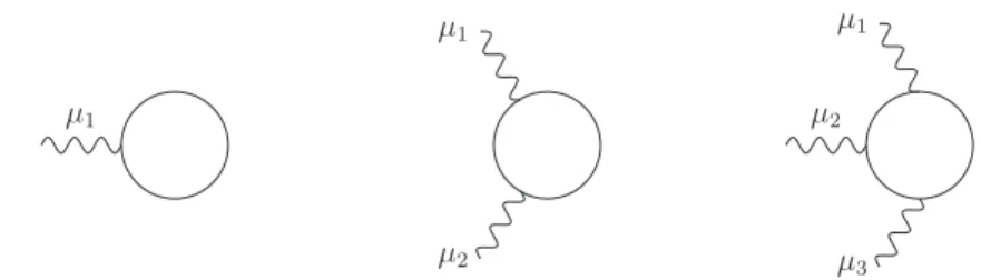
Feynman diagrams. To this end we use IReg in the integrals needed in the diagrammatic proof, and study under which conditions the Ward Identities are respected. In what follows we use a pictoric representation (figure 3.2) of the Ward Identities as in [43], namely:
kνA νµ1=
µ1 k
kνB νµ1µ2 =
µ1
µ2
k
+ µ1
µ2
k
kνC
νµ1µ2µ3=
µ2
µ1
µ3
k
+ µ2
µ1
µ3
k
+ µ2 µ1
µ3
k
Figure 3.2: Pictoric representation of QED Ward identities kνA
νµ1 = 0, kνB
νµ1µ2 = 0, and k
νC
νµ1µ2µ3 = 0. Diagrams with more than four external
Explicitly,
kνAνµ1 =T r Z
p
γµ1
1
/p+α/+k/
/ k
1
/p+α/
, (3.24)
kνBνµ1µ2 =T r Z
p
γµ2
1
/p+β/+k/+/q
γµ1
1
/p+β/+/k
/ k
1
/p+β/
+T r
Z
p
γµ2
1
/p+β/+k/+/q
/ k
1
/p+β/+/q
γµ1
1
/p+β/
, (3.25)
kνCνµ1µ2µ3 =T r Z
p
γµ3
1
/
P +/k+Q/
γµ2
1
/
P +/k+/q1
!
γµ1
1
/ P +k/
/ k 1 / P
+T r
Z
p
γµ3
1
/
P +/k+Q/
γµ2
1
/
P +/k+/q1
!
/
k 1
/ P +/q1
!
γµ1
1
/ P
+T r
Z
p
γµ3
1
/
P +/k+Q/
/ k 1 / P +Q/
γµ2
1
/ P +/q1
!
γµ1 1 / P , (3.26)
where P ≡p+δ, α, β, and δ are arbitrary routings and Q/ ≡/q1+/q2. By using IReg we finally obtain:
kνAνµ1 =−4Γ (1,2)
2 kµ1 + 4
Γ(10,2)−4Γ(10,4) k·(k+ 2α)αµ1 + (k+α) 2k
µ1
,
(3.27)
kνBνµ1µ2 =−4
Γ0(1,2)−4Γ0(1,4) gµ1µ2k·(k+q+ 2β) +kµ1(k+q+ 2β)µ2+
+kµ2(k+q+ 2β)µ1
, (3.28)
kνCνµ1µ2µ3 = 4
Γ0(1,2)−4Γ0(1,4) gµ1µ2kµ3 +gµ1µ3kµ2 +gµ2µ3kµ1
. (3.29)
with surface terms defined in eq. (2.10). We notice that Ward identities are fulfilled provided
Γ(12,2) = Γ0(1,2) = Γ(10 ,4) = 0. (3.30) Thus by adopting an abelian gauge invariant regularization (setting surface terms to zero) one automatically preserves MRI.
µ1
µ1
µ2
µ2
µ1
µ3
Figure 3.3: Diagrams needed in the diagramatic proof of abelian gauge invari-ance.
Performing the calculation one notices that MRI is respected if
Γ(12,2) = Γ0(1,2) = Γ(10 ,4) = 0, (3.31)
which are the same conditions to preserve the Ward identities. Therefore we conclude that MRI is a necessary and sufficient condition to preserve abelian gauge symmetry at arbitrary loop order. This should be emphasized that the previous conclusion regards a theory free of chiral couplings (proportional to γ5). This feature can be easily seen in the Adler-Bardeen-Bell-Jackiw (ABJ) chiral anomaly in which the axial Ward identity must be violated if momentum routing invariance is to be respected.
symmetrized, as already mentioned in [46]. Explicitly we have
1
4Tr [γ5γαγµγβγνγργλ] =ǫαµβνgρλ−ǫαµβρgνλ+ǫαµνρgβλ−ǫαβνρgµλ+ +ǫµβνρgαλ−ǫλαµβgρν+ǫλαµνgρβ−ǫλαβνgρµ+ǫλµβνgρα−ǫλραµgνβ+
+ǫλραβgνµ−ǫλρµβgνα+ǫλρναgµβ −ǫλρνµgαβ +ǫλρνβgαµ. (3.32)
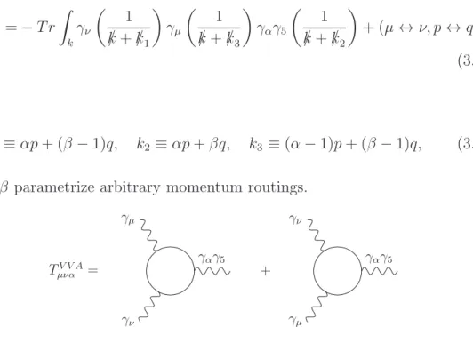
After this comment, we proceed to the evaluation of the anomaly itself. The relevant diagrams are depicted in figure 3.4, whose amplitudes are given by
TµναV V A=−T r
Z
k
γν
1
/ k+/k1
γµ
1
/ k+/k3
γαγ5
1
/ k+/k2
+ (µ↔ν, p↔q),
(3.33)
where
k1 ≡αp+ (β−1)q, k2 ≡αp+βq, k3 ≡(α−1)p+ (β−1)q, (3.34)
and α,β parametrize arbitrary momentum routings.
TV V A µνα =
γµ
γν
γαγ5
+
γν
γµ
γαγ5
Figure 3.4: Diagrams of the Adler-Bardeen-Bell-Jackiw chiral anomaly with an arbitrary momentum routing.
Using now eq. (3.32) and the rules of IReg one arrives at the vector and axial Ward identities, which cannot be satisfied simultaneously
pµTµναV V A = 4i(α−β−1)Γ(10,2)ǫµναβpµqβ
qνTV V A
µνα =−4i(α−β−1)Γ
(1,2)
0 ǫµναβqνpβ
(p+q)αTµναV V A = 8i(α−β−1)Γ(10,2)ǫµναβpαqβ−
1
2π2ǫµναβp
A comment is in order to clarify the interplay between surface terms and MRI in the presence of anomalies. We notice that by setting Γ(10,2) to zero one imple-ments MRI since the Ward identities will be independent of α and β. However, this choice for Γ(10,2) strikingly spoils the democracy that the calculation scheme should preserve between the vector and axial Ward identities which must be fixed on physical grounds [42]. In other words, the surface term should be left arbitrary and a new constraint should be imposed on the theory. In the case of the ABJ chiral anomaly, the pion decay into two photons (experimental data) requires the conservation of the vector current. Therefore, the surface term should be null which represents preservation of MRI. Once again, we notice the connection be-tween abelian gauge symmetry (represented by the vector Ward identity in this case) and MRI.
3.3
Momentum Routing Invariance in the
con-text of scalar field theories
Having demonstrated that the imposition of momentum routing invariance au-tomatically preserves abelian gauge symmetry to all-orders,, we wonder which would be the consequences of MRI breaking in a theory with low symmetry con-tent. We study masslessφ3
6 theory by calculating itsβ-function at two-loop order
[34]. The Feynman diagrams we will need are depicted in figure3.5.
p
k1
p p k1 k2 p p k2
k1
p
Since we want to stress the connection between surface terms and MRI, we will use an arbitrary momentum routing in the diagrams above. However, following the calculation outlined at [34], one can easily see that only the momentum routing of the subgraph of the third and sixth diagrams will affect the coefficients of the β-function at two-loop order. Thus, we will use the following convention
p1 k1
p2 p1 k1 k2
p2 3×
p1 k1 k2
p2 3×
p1 k2 k1
p2
Figure 3.5: Diagrams contributing up to two-loop order of φ3
6 theory. Ξ stands
for two-point functions and ∆ stands for three-point ones.
p k2+αk1
k1 p
p1 k2+αk1 k1
p2
Figure 3.6: Diagrams whose choice of momentum routing may affect the coeffi-cients of the β-function at two-loop order.
and vertex
Ξ =−g2
"
p2
6I
(1)
log(λ2)
#
+ig4
("
− 2954b6 − (3α
2−3α+ 1)Γ(1,2) 0
9
!
Ilog(1)(λ2)+
+5b6 18I
(2)
log(λ2)
#
p2
)
+ terms that do not contribute to the β-function, (3.36)
∆ =−g3
"
Ilog(1)(λ2)
#
+ig5
"
5b6
2 I
(2)
log(λ
2) −
17b6
3 −(3α
2
−3α+ 1)Γ(10,2)
Ilog(1)(λ2)
#
+ terms that do not contribute to the β-function, (3.37)
where b6 ≡ −1
2
i
(4π)3.
With these results, the β-function can be calculated yielding
β=− 3g
3
4(4π)3 −
125g5
144(4π)6 +
ig5[12(α2−α) + 5] Γ(1,2) 0
6(4π)3 +O(g
6). (3.38)
mass independent scheme are universal. We notice that we obtain the universal values of the β-function only if we set Γ(10,2) = 0, which is the same condition to preserve MRI. On the other hand it becomes also clear from our expression for the beta function that should the surface term be non-vanishing the two loop universal beta function coefficient would be momentum routing dependent (in our case would depend onα). Therefore, we conclude that even in a theory with poor symmetry content such as φ3
6, momentum routing invariance is important since
it is responsible for the preservation of the universal values of the β-function.
Concluding Remarks
Chapter 4
(Un)determined finite
regularization dependent
quantum corrections: the Higgs
decay into two photons and the
two photon scattering examples
Introduction
many doubts on the statements presented on [49]. Other authors used Cutoff Regularization [56, 57] obtaining the same result of [49] thus concluding that such regularization is unpredictive if one works on the unitary gauge. Other works were devoted to the discussion of the decoupling theorem [58,59] questioning the reliability of the predictions made on [49].
Contemporary to Gastmans et al. work, another paper questioned an old-stabilished result in the literature: the cross section of the two photon scattering [60]. Once again, doubts were raised against the use of regularization. A work followed in which this issue was explained [61] in the framework of Dimensional Regularization and Paulli-Villars recovering the old results found in the literature [62,63].
of divergent integrals. Therefore, instead of just adding the result of a differ-ent method to the literature we intend to show that the discussions presdiffer-ented in [53,54, 55, 56,57] can all be explained using just one framework.
4.1
A general view of regularization dependent
integrals
In this section we discuss on general grounds the issue of regularization dependent integrals leaving the physical calculations of the Higgs decay as well as of the two photon scattering to subsequent sections. Proceeding this way we hope to set the subject, both from a conceptual and technical point of view, in a consistent and self-contained way allowing a clearer discussion of the examples just cited.
As is well known Quantum Field Theoretical Feynman diagram calculations involve integration in the momentum loops which must be regularized due to ultraviolet and sometimes infrared divergences. The renormalization program consistently redefines physical degrees of freedom order by order in perturbation theory. Symmetry requirements may either be ensured by an invariant regular-ization or imposed as constraint equations as dictated by Ward-Slavnov-Taylor identities order by order in the loops. Yet a little calculational tedious, the latter procedure is perfectly sound for both anomaly free theories and models in which the quantum symmetry breaking mechanism is well known.
A plethora of regularization schemes have been constructed to be used where gauge invariant Dimensional Regularization may fail, namely in the so called dimensional specific theories among which supersymmetric, chiral and topolog-ical quantum field theories figure in. A natural question would be which basic properties should a method that does not recourse to analytical continuation in the space-time dimension should retain in order to be invariant. We start by illustrating with simple examples following [67]. Let ∆ be the superficial degree of divergence of a n loop integral where the momentum kn runs. Consider the
following 1-loop ∆ = 2 integrals,
A=
Z
k
k2
and
B =Iquad(m2) +m2Ilog(m2), (4.2)
where Rk ≡ R d4k/(2π)4 and we recover the standard notation in Implicit
Regu-larization
Ilog(m2)≡
Z
k
1
(k2−m2)2, and Iquad(m 2)
≡
Z
k
1
(k2 −m2). (4.3)
We expect A=B be guaranteed by any regularization procedure. However this is not the case. Proper-time regularization [68] for instance, introduces a cutoff Λ after Wick rotation via the following identity at the level of propagators
Γ(n) (k2+m2)n =
Z ∞
0
dτ τn−1e−τ(k2+m2) →
Z ∞
1/Λ2
dτ τn−1e−τ(k2+m2)
. (4.4)
Thus it is trivial to obtain within the proper-time method that A6=B since
AΛ = −
2i
(4π)2
Λ2−m2ln
Λ2 m2
, (4.5)
whereas
BΛ= −2i (4π)2
Λ2
2 −m
2ln
Λ2 m2
. (4.6)
On the other hand it is straightforward to show that standard Dimensional Reg-ularization leads to A = B. To circumvent such discrepancy the authors of [67] define a n-dimensional integral
I(α, β) =
Z n
k
1
(αk2+βm2), (4.7)
for α and β arbitrary in order to write
A=− ∂
∂αI(α, β)
α=β=1,n=4, (4.8)
and
B =I(α, β)
α=β=1,n=4+ ∂
∂βI(α, β)
Then resorting to proper time regularization one gets
I(α, β)Λ =α−n/2
Z n
k
1
(k2−βm2) =
−αn/2i
(4π)2
Λ2−βm2ln
Λ2 m2
, (4.10)
from which is obtained
AnΛ = −i (4π)2
n
2Λ
2 − n
2m
2ln
Λ2 m2
, (4.11)
and
BΛn = −i (4π)2
Λ2−2m2ln
Λ2 m2
. (4.12)
Whilst keeping n = 4 violates A = B, the choices n = 4 in the term ∝ ln Λ2
and n = 2 in the term ∝Λ2 lead A to coincide withB at regularized level. Yet
arbitrary the authors consider such prescription, which is generalizable to other integrals in Feynman amplitudes, a concrete realization for a four dimensional regularization. They claim that Veltman in [69] already notices that quadratic divergences are associated with n = 2 whereas logarithmic divergences have to be treated in n = 4 in Dimensional Regularization. Other authors have used a similar approach [70, 71, 72].
Let us now consider another related example. Consider the effect of a shift in the integration variable in a four dimensional integral. As well known such shifts accompany surface terms in more than logarithmically divergent integrals. Their value is highly regularization dependent. For instance take the difference between two linearly divergent integrals for ω = 2
∆1 =
Z 2ω
k
kµ
[(k−p)2−m2]2 −
Z 2ω
k
(k+p)µ
[k2−m2]2. (4.13)
Clearly ∆1 = 0 in Dimensional Regularization because no surface terms
accom-pany shifts in the integration variable. In [65] the authors generalize the proce-dure adopted by Jauch and Rohrlich in [73] to evaluate ∆1 for ω exactly equal
Regu-larization. By defining
Iµ2n1...µ+1,r2n+1 =
Z 2ω
k
Q2n+1
j=1 kµj
[(k−p)2−m2]r, and J
2n+1,r µ1...µ2n+1 =
Z 2ω
k
Q2n+1
j=1 (k+p)µj [k2−m2]r ,
(4.14) in [65] is shown that whilstI =Jfor 2ω+2n+1−2r <1, if 2 >2ω+2n+1−2r >1 then
Iµ2n1...µ+1,r2n+1 −Jµ21n...µ+1,r2n+1 = −i(2π)
4πωG
n,2n+1(p)
Γ(ω) δr,ω+n, (4.15)
with
Gn,2n+1(p) =
gµj1µj2 . . . gµj2n−1µj2npµj2n+1σ
j1...j2n+1
Γ(ω)−1Γ(ω+n+ 1)n!22n , (4.16)
and
σj1...j2n+1 =ǫj1...j2n+1(−)sign(ǫ). (4.17)
For n= 0 we immediately obtain
∆1 = −
iπ2(2π)4
2 δω2pµ. (4.18)
A similar expression may be obtained for more than linearly divergent variable shifted integrals. It is immediate from above that the kronecker delta signs a discontinuity in the dimensionalityω. The authors use these results to back up an integer dimensional regularization called Preregularization where the freedom of momentum routing in the loops is chosen to cancel out some surface terms in order to preserve Ward identities in chiral anomalies or supersymmetry [40, 74, 75]. A relevant question, given that shifts of integration variables are regularization dependent, would be to verify whether the argument could be turned the other way around, namely to exploit the consequences of momentum routing invariance over regularization schemes. Some technicalities deserve attention. Symmetric integration in n (integer) dimensions, namely kµkν → gµνk2/n under integration
in k for divergent integrals does not hold in general and has been a source of disagreements in loop calculations as well discussed in [39] in the context of CPT violation in quantum field theory and used in [49] to study Higgs’ s decay in two photons. In particular symmetric integration was used in [73] to evaluate ∆1.
to deal with these ambiguities. As showed there, there is the appearance of the following objects
Υµν0 ≡
Z d
k
∂ ∂kµ
kν
(k2−m2)d2
=d
"
gµν
d Ilog(m
2)−Iµν log(m2)
#
, (4.19)
and
Υµν2 ≡
Z d
k
∂ ∂kµ
kν
(k2−m2)d−22 = (d−2)
"
gµν
(d−2)Iquad(m
2)
−Iquadµν (m2)
#
. (4.20)
The surface terms Υ’s are regularization dependent terms which however can be shown to be physical meaningful and therefore be fixed. In the process of reducing the set of loop integrals to basic divergent integrals it can be shown that the vanishing of surface terms expressed by the Υ’s reflects momentum routing invariance in the loops of a Feynman diagram [18, 66]. Attributing spurious values to such surface terms is the root of quantum symmetry breakings by reg-ularizations. Once we attach a physical meaning to them, as it is proposed in the Implicit Regularization program we may regularize infinities in a regulariza-tion independent fashion because the renormalizaregulariza-tion constants can be defined in terms of basic divergent integrals themselves.
As for the examples we presented earlier, it is immediate that A =B within our approach because summing and subtracting m2 in the numerator of A leads
to B. Whenever even powers of internal momenta appear in the numerator, one can always make use of such artifice to avoid ambiguous symmetric integration [23]. As for ∆1 in equation (4.13) one obtains within Implicit Regularization
∆IR
1 = Υ
µν
0 pν. (4.21)
4.2
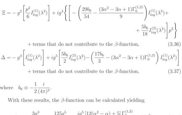
Higgs decay into two photons
H
p1+p2
α α
k+χ1
k+χ3
β γ µ ν ρ σ p1 p2
k+χ2
γ γ W+ W+ W+ M1 H
p1+p2
α α
k+χ1
k+χ3
β γ ν µ ρ σ p2 p1
k+ ¯χ2
γ γ W+ W+ W+ M3 H
p1+p2
α α
k+χ1
k+χ3
β γ µ ν p1 p2 γ γ W+ W+ M2
Figure 4.1: Diagrams with arbitrary momentum routing χ
since we want to study how the final amplitude depends on it.
The sum of the three diagrams can be symplified to the expression (the strat-egy is to group the terms of the integrand in order ofM−n
w and consider that the
external photons are onshell p2
i = 0 and p21+p22 =Mh2)1
M =ie2gMw
h
Mµν(a)+Mµν(b)+Mµν(c)i(ǫ1µ)∗(ǫ2ν)∗+ (p1 ↔p2, µ↔ν), (4.22)
Mµν(a) =− 4
M2
w
h
gµν(p1)α(p2)βIαβ(3)+ (p1·p2)Iµν(3)−(p1)ν(p2)αIµα(3)−(p2)µ(p1)αIνα(3)
i + + 2 M2 w h
gµν(p1·p2)−(p2)µ(p1)ν
i
I2(3), (4.23)
Mµν(b)=
Z
k
3(gµνk2−4kµkν)
(q2
1 −Mw2)(q22−Mw2)(q32−Mw2)
, (4.24)
Mµν(c)= 6gµν
h
(p1·p2)I0(3)−(p1)αIα(3)−
M2 w 2 I (3) 0 i
+ 6h2(p1)νIµ(3)−(p2)µ(p1)νI0(3)
i
,
(4.25)
I0(3),2,µ,µν =
Z
k
1, k2, k
µ, kµkν
(q2
1−Mw2)(q22 −Mw2)(q32−Mw2)
. (4.26)
As one may notice, onlyMµν(a)and Mµν(b)contain divergent terms. At this point
we must choose a regularization in order to deal properly with such terms. We employ IReg since all regularization-dependent objects (surface terms) can be consistently treated allowing a clear discussion about ambiguities as will be seen
1We defineq
i=k+χi, ¯qi=k+ ¯χi andR k
below. Therefore the first term is given by
Mµν(a)=
(p2)µ(p1)ν−gµν(p1·p2)
M2
w
"
i
16π2 −2Γ (1,2) 0
#
. (4.27)
The first point to be noticed is that this term is gauge invariant and, in general, ambiguous since it depends on a surface term. Another feature is that it is proportional1 to τ0 which furnishes us a clue that it may be the term missing
on [49]. In fact, if one performs a symmetric regularization in four-dimensions (by replacing kµkν → gµνk2/4) it will be null. In other words a 4-dimensional
regularization that resorts to such substitution is evaluating the surface term to a precise value in this case i/32π2. On the other hand, if one uses Dimensional
Regularization the surface term will vanish which furnishes anon-nullamplitude in the limit τ−1 → 0. In the framework of IReg there is no reason a priori to
favour one of these two values since we are dealing with ambiguous objects in nature. From our perspective physical conditions, other than the regularization method, should constrain the value the surface term should assume. In general, one such condition is to impose gauge invariance, however, since this term is
already gauge invariant, this consideration will not fix it. Therefore, we should leave it arbitrary and proceed with the calculation of the amplitude for now. The sum of the two last terms is2
Mµν(b)+Mµν(c) = i 16π2M2
w
(p2)µ(p1)ν −gµν(p1 ·p2)
"3τ−1
2 +
3(2τ−1 −τ−2)f(τ)
2
#
+gµν(p1·p2)
3τ−1
2M2
w
Γ(10 ,2)
!
. (4.28)
1We defineτ= M2
h
4Mw2
2Where we define
f(τ) =
arcsin2(√τ) for τ≤1,
−14 "
ln1 + √
1−τ−1
1−√1−τ−1 −
iπ
#2
Readily one may notice the appearance of another surface term due to Mµν(b)
which explicitly breaks gauge invariance. Since there are no other terms to con-sider, one should impose gauge invariance as a physical condition that the whole amplitude should fulfill. Thus the otherwise arbitrary surface term must assume a precise value which in our case is null. This choice also fixes the surface term appearing in (5.54) since in the framework of IReg there is no distinction be-tween surface terms coming from integrals with the same degree of divergence and the same Lorentz structure. This approach is different from the one found in [56] where a cutoff scheme is used and it is claimed that the ambiguities can be parametrized by different boundary conditions for the integrals appearing in (5.54) and (5.55).
After all these considerations we obtain the amplitude for the Higgs decay into two photons in the framework of IReg
M =− e
2g
16π2M
w
(p2)µ(p1)ν −gµν(p1·p2)
2 + 3
τ +
3
τ
2− 1
τ
f(τ)
(ǫ1µ)∗(ǫ2ν)∗,
(4.29)
which agrees with previous one found in the literature [50, 51, 52].
In the time this work was been written, another paper devoted to this decay appeared [76]. Their authors have a point of view similar to ours in the sense that ambiguities should be fixed on physical grounds 1. They use the equivalence theorem as well as the conservation of charge as inputs that their amplitude must fulfill. Since these are consequences of gauge invariance there is no surprise that just the imposition of such requirement gives us an unambiguous result.
Another interesting point discussed there is the role played by momentum routing freedom. From their point of view the loop-momentum of the three dia-grams must be chosen in a particular way as to reduce the superficial degree of divergence of the amplitude to a logarithmic one.2 However, from our point of
1It should be emphasized that their definition of the ambiguity is more closely related to
the one found in [42]. We, on the other hand, define it by (4.19) which is more closely related to the preservation of Abelian gauge invariance [66]
2They find that all three diagrams must contain the same momentum routing. Therefore it
view momentum routing invariance (MRI) is a symmetry that must be respected since it is connected with Abelian gauge invariance as well as supersymmetry preservation [66]. The importance of this statement is particular clear if, instead of considering the calculation of the whole amplitude, one evaluates each diagram
individually. Following the reasoning of [66] one founds out that momentum routing dependent terms will arise always multiplied by arbitrary-valued objects (surface terms). Therefore, since individual diagrams are not supposed to be gauge invariant, the only symmetry left in order to fix the ambiguities is de-manding momentum routing invariance. As can be seen, we could have adopted this approach from the beginning of our work avoiding completely the discussion of gauge invariance (since the two symmetries are connected it is not a surprise that the surface terms must be null in both cases). However, in order to make contact with the literature we performed the calculation of the whole amplitude with the same routing for all three diagrams which evidently is not the more general situation. Therefore, it is not a surprise that our result is independent of the momentum routing χ1 even though we still have an ambiguity expressed by
Γ(10 ,2).
4.3
Two photon scattering
In this brief section we would like to comment on the result found on [60]. As in the case just analized, the problem lies on divergent integrals which appear as intermediate steps of the calculation. Explicitly we have [61]
Aµνρσ =
Z
k
m4Sµνρσ
1 + 2m2(2S
µνρσ
2 −k2S
µνρσ
1 )
(k2−m2)4
+
Z
k
24kµkνkρkσ+ (k2)2Sµνρσ
1 −4k2S
µνρσ
2
(k2−m2)4 , (4.30)
where
S1µνρσ =gµνgρσ+gµρgνσ +gµσgρν,
As can be readily seen, the integral above is divergent, thus ambiguous. Such statement is particularly clear in the framework of IReg since it is evaluated to (Γ(10,2)−4Γ0(1,4))S1µνρσ where Γ(10,i) is a surface term coming from an integral with Lorentz structure kν1· · ·kνi as defined in chapter 2. Therefore, there is no pre-ferred value this integral should assume, it should be left arbitrary being fixed by the imposition of physical conditions. As discussed in [61], a non-null value forAµνρσ implies the breaking of gauge invariance which means the surface terms
must obey Γ(10,2) = 4Γ(10,4) in order to respect such symmetry. Thus, there is no ambiguity left on the final amplitude which as expected agrees with previous re-sults found in the literature [61]. In summary, as in the case of [49], the authors of [60] performed a symmetric regularization on the integral above which in turn gave a precise value to the surface terms (Aµνρσ = (i/96π2)Sµνρσ
1 ). Such choice
resulted in a different cross section for the two photon scattering than the one found previously in the literature [62, 63]. However, since the integral is ambigu-ous in nature there is no reason to assume a precise value for the surface terms which must be fixed on physical grounds.
Concluding remarks
Chapter 5
Guises and Disguises of
Quadratic Divergences
Introduction
The Higgs boson discovery at the LHC [47,48] (mH ≈125GeV) as well as the lack
of data supporting on low energy extensions to the standard model (SM) such as supersymmetry (SuSy) has renewed the interest in possible explanations for both the electroweak hierarchy and the naturalness problem. These issues are related to a certain extent to how we interpret quadratic divergences in field theories. Two kinds of hierarchy problems arise in the SM [77]. The most commonly referred one, which we will simply call hierarchy problem, is related to the large radiative corrections to the Higgs mass stemming from quadratic divergences in the cutoff which supposedly cancel against the tree level value to a very high precision at the weak scale. Consequently the Higgs mass becomes quadratically sensitive to a cutoff scale Λ. On the other hand the gauge hierarchy problem has to do with logarithmic divergences which determine the running of the coupling constants: if on one level the scale that characterizes the symmetry breaking of the GUT which unifies quantum chromodynamics and electroweak theory [78] is 1014GeV, on the
other level the electroweak symmetry breaking scale is about 102GeV. Explaining
divergences of a renormalizable theory which are multiplicatively renormalized, lead to a subtractive renormalization of the Higgs boson mass. Thus the hierarchy problem is reduced to the naturalness of such subtraction. SuSy avoids such subtractive renormalization and would solve the technical naturalness of the SM should SuSy particles be sufficiently light.
It is important to remark that contrarily to the interpretation in ultraviolet (UV) complete theories, quadratic divergences cannot be excused away as an artifact of the regularization procedure by simply adopting dimensional regular-ization, for instance. Taking the SM as the low energy limit of a more complete theory, a cutoff must be introduced to set a landmark in which new degrees of freedom appear. Notice that the meaning of a cutoff Λ is twofold: it can play the role of the UV cutoff of an UV complete theory (Λ→ ∞) or a cutoff in an effective theory at which new degrees of freedom appear (merging scale). For example, for low energy models of QCD, Λ ≈ 1GeV, as quarks and gluons are not well defined degrees of freedom in this region [70]. Evidently, for both the ultraviolet complete and the effective theory, naive subtraction of quadratic divergences has no effect upon the low energy dynamics. However in drawing conclusions about new physics, such subtraction becomes a subtle and relevant issue.
However, as pointed out in [80], the absence of quadratic divergences does not fully solve the hierarchy problem. The SM must also be UV completed at the scale Λ by a theory without quadratic divergences. Thus the problem also passes by at which scale a complete theory (say, SuSy) appears. That is because a matching of the parameters of the high energy and low energy physics ought to guarantee light Higgs mass parameters at the merging scale. Such fine tuning would be avoided only if Λ≈103GeV [80].
Different constructions, differing by their level of sophistication, have appeared in the literature to explain away the role played by quadratic divergences in the naturalness problem, given that new physics has not been found at LHC with
√