Abstract—Most object tracking trees are established using the predefined mobility profile. However, when the real object’s movement behaviors and query rates are different from the predefined mobility profile and query rates, the update cost and query cost of object tracking tree may increase. To upgrade the object tracking tree, the sink needs to send very large messages to collect the real movement information from the network, introducing a very large message overhead, which is referred to as adaptation cost. The Sub Root Message-Tree Adaptive procedure was proposed to dynamically collect the real movement information under the sub-tree and reconstruct the sub-tree to provide good performance based on the collected information. The simulation results indicates that the Sub Root Message-Tree Adaptive procedure is sufficient to achieve good total cost and lower adaptation cost.
Index Terms—wireless sensor network, object tracking, dynamic object tracking tree
I. INTRODUCTION
ensor networks are used in environmental monitoring, military surveillance and home and industrial security. With the recent advances in embedded micro-sensing technologies, the sensors are smaller, cheaper and more intelligent. These sensors are equipped with wireless interfaces that allow communication with other sensors in order to form a network. The wireless sensor has the ability to collect, process and store information from its surroundings and can be accessed from the Internet.
With the advances in embedded micro-sensing technologies and sensing and communication technology integration, large
Manuscript received Oct. 18th, 2012.
This work was supported by the National Science Council of Taiwan, R.O.C. under Grant NSC95-2221-E-216-039, NSC96-2221-E-216-010, and NSC97-2221-E-259-036.
Min-Xiou Chen is with Department of Computer Science and Information Engineering, National Dong Hwa University, Hualien, Taiwan, R.O.C. (phone: 886-3-8634054; e-mail: mxchen@ mail.ndhu.edu.tw).
Che-Chen Hu, was with Department of Computer Science and Information Engineering, Chung Hua University, Hsinchu, Taiwan, R.O.C. (e-mail: [email protected]).
scale wireless sensor networks can be developed with a great number of compact sensors. Numerous researchers have produced wireless sensor networks, including routing and transport protocols [1]-[3], physical and medium access layers [4]-[6] and localization and positioning applications [7]-[9].
Another important research into wireless sensor networks is object tracking [11]-[21][24][25]. The key functions involved in object tracking include detection, identification, classification, location estimation and monitoring. A large number of sensors will be deployed to detect moving objects and report on the object’s location to the sink, who is the processing node responsible for collecting the object location information from the sensors.
Figure 1 shows an object tracking scenario. Wireless sensors are deployed at road intersections in the city. Each sensor has the ability to detect vehicles and communicate with its neighbor sensors. The sink acts as a traffic information center to manage and monitor traffic. When a vehicle (car 2) moves from node E’s sensing range into node D’s sensing range, node D will detect the vehicle and report to the sink, who will be able to know the location of that vehicle. Node E will report a departure message for car 2 to the sink. All this messages from sensor will result in a lot of information. Moreover, due to the limitation of the sensor’s power, the sensors near the sink, such as node A and
Min-Xiou Chen,
Member, IEEE
, and Che-Chen Hu,
Efficient Dynamic Adaptation Strategies for
Object Tracking Tree in Wireless Sensor
Network
S
B will quickly use up their batteries (because that these nodes near the sink needed to forward the packets sent from those nodes on the far side), and the wireless sensor network will be partitioned. Therefore, designing effective data collection architecture is an important research topic. Some researches [14]-[21] proposed constructing a collection architecture using a tree according to the mobility profile, which is generated according to the mobility model. Nevertheless, the actual object movement behavior may not match the mobility model and this difference may affect the performance of the collection architecture. Therefore, the Message-Tree Adaptive procedure (MTA) was proposed in [22] to dynamically adapt the object-tracking tree.
The problem with the MTA procedure is that it incurs a lot of message overhead to improve the update cost of the object tracking tree. Moreover, the impact of query cost was not considered. Therefore, the Sub Root Message-Tree Adaptive procedure is proposed to achieve good performance regardless of the object’s actual movement behavior and to have smaller objects’ query rates with lower message overhead.
The rest of this paper organized as follows. The related literatures are discussed in Section 2. Section 3 proposes the network model, a Sub Root Message-Tree Adaptive procedure and shows simulation results in Section 4. The conclusions are in Section 5.
II. RELATED WORK
The proposed researches on wireless sensor network target tracking can be grouped into four main approaches, cluster-based tree [3][11]-[12][23], prediction-based [13][23], hierarchy-based tree [14]-[21] and agent-oriented approach for tracking application[24][25].
The cluster-based tree organizes all sensors into several clusters and an election of cluster heads will determine which node takes responsibility for collecting the object information within the same cluster and report that information back to the sink. This node is called the cluster head. When the distance between the cluster head and sink is more than one hop, a multiple hop path is created between the cluster head and sink. Due to the limitation in sensor power, the sensors near the sink will use up their batteries and the wireless sensor network will be partitioned.
The LEACH algorithm proposed in [3] builds a cluster-based tree to track object in two steps. The first step is the set-up,where a local cluster head is randomly chosen. The local cluster heads will collect the object information sent from the sensor nodes and forward the object information to the sink in the second phase. However, the LEACH algorithm concentrates only on finding an efficient way to forward the object information to sink but does not find the robust and reliable object tracking tree in an energy efficient manner.
Another dynamic cluster structure was proposed in [11] to efficiently collect the object information. In that paper, the boundary nodes located near the tracking object must be identified. The dynamic cluster structure then collects the
boundary nodes information and the boundary nodes report the tracking information to the sink through the cluster heads. Jin et al. in [12] proposed a new dynamic clustering mechanism to reduce the transmission power consumption, lower the transmission cost, and lower the transmission fault rate, which is constructed based on object movement and modified according to the object’s routing information and sensor node information in order to reduce the transmission power consumption and lower the transmission cost.
The second main group comprises the prediction-based approaches, which add prediction models to construct the object tracking tree. The heterogeneous tracking model (HTM) for object tracking was proposed in [13]. The variable memory Markov (VMM) concept was introduced to predict the patterns of moving objects and used these patterns to construct the cluster tree. However, the computation necessary for the VMM is very high, and when the prediction patterns do not match, the performance of the cluster tree will decay.
The main characteristics of agent-oriented approach are to use the autonomous software agents to interact with other agents, and to use higher level programming languages and methodologies that allow the adoption of flexible mobile agents’ software. The major objective of the agent-oriented approach is to design a high-level language and virtual machine technology to change or update these agent functions in order to provide an intelligent sensor network with lower system overhead and higher system performance.
The major drawback of the cluster-based tree is the high transmission power consumption, which leads to the third main approach, the hierarchy-based tree-structuring algorithm. One of these algorithms, referred to as “drain-and-balance (DAB)” tree, proposed in [14] can reduce the drawbacks from the prediction based approaches.. The DAB tree is a binary logical tree whose root is the sink and is constructed based on the event rate cost. All the leaves of the tree have the ability of tracking an object and reporting the collected information. The intermediate nodes can store and forward these object information, but cannot track the object. The data aggregation technology was introduced, and these object information will be forwarded to the lowest common ancestor of these two sensor nodes which are the leaves and track the object, allowing for some messages not to be sent to the sink. With the data aggregation technology, the power consumption and transmission can be reduced.
introduces the query cost reduction (QCR) method to reduce the query cost. To reduce the query cost and communication cost, the multi-sink tree was proposed in [16].
In [17][18], the authors also proposed an object tracking tree to track an object in a wireless sensor network. Although the computation complexity of these solution is better than that of DAT, but the performance of these strategies cannot be better than that of the DAT, because these papers want to find a good tree with a lower computation complexity.
In [19], the authors proved that establishing an object-tracking tree with the minimum update cost is a NP-complete problem and. proposed the addition of a shortcut mechanism into the existing object-tracking tree to reduce the update and query costs.
In [20], the tree adaptation procedure (TAP) was proposed to improve the query cost of the object tracking tree, which is a bottom-up approach and selects a candidate node based on the bottom-up rule. The TAP computes the update cost using the edge connected to the target node, but was not included in the object tracking tree. When the update cost of the modified object tracking tree is better than that of the original object tracking tree, the modified object tracking tree will be set as the new object tracking tree. The TAP will compute the update cost for the modified object tracking tree until all nodes except the sink have been considered. The simulation results show that the TAP application achieves good performance, and can be better than that of DAT.
All the hierarchy based mechanisms require an input mobility profile that describes the object crossing rate between neighboring sensors, which can be obtained based on historical statistics. Nevertheless, the real movements of physical objects may be very different to the mobility profile. In [21], the authors proposed a mathematical model that generates a mobility profile based on stochastic process theory, which is useful when the object mobility pattern is unknown.
As discussed above, the object tracking performance may be worse when the mobility profile is not correct. The message-tree adaptive (MTA) procedure was proposed to dynamically adapt the object-tracking tree [22]. This procedure can dynamically
Fig. 3. An Example of Object Tracking Tree. In (a) we see the original graphic; in (b) Object tracking treee is constructed according to DAT and update cost is 1605; in (c) the event rate of w(F, J), w(H, I) and w(E, G) are changed update cost is and update cost becomes to 1986; in (d) the update cost of the reconstructed object tracking treee is 1958.
adapt the object-tracking tree to achieve good performance and to suit to the real environment. However, the MTA procedure causes a lot of message overhead to improve the object tracking tree, and the impact of query cost was not considered in the paper.
In [23], the authors proposed an information-based adaptive target algorithm based on the dynamic cluster and target prediction mechanism, which can adjust the information collection distance and time interval, depending on the target object’s velocity, acceleration and angle variations. It also adjusts the time interval of each cluster prediction formation, depending on the target object’s velocity and angle variations. The simulation results show that the proposed algorithm has better tracking precision and lower energy consumption.
However, these approaches cause a lot of message overhead to collect information and announce the update structure. The impact of query rate changed was not considered in these approaches. Thus, in next session, we will propose an approach to adapt the tree structure according to the real traffic information and query rate with lower message overhead.
III. SYSTEM ARCHITECTURE
A. Network Model
Consider a network that consists of a set of wireless sensor node deployed in a closed field. Assume that these nodes have unique identifications and are time-synchronized. A special node, the sink, will work as the gateway to the wireless sensor network from the outside world. After deployment, the sink will know each sensor node’s location and each sensor node will report the arrival information to the sink when it detects an object moving into its area and send the departure information to the sink when the objects moves out of its area. In order to avoid redundant reports, the simple nearest-sensor tracking model was introduced, in which only the sensor node that receives the strongest signal from an object is responsible for tracking the object.
Therefore, in the deployment region the sensing field area of each sensor node can be modeled using a Voronoi graph [10], as depicted in Figure 2(a). When node i and node j share a common border in the Voronoi graph, these nodes are called neighbors. A line between node i and node j can be drawn as the boundary, indicating the area where each sensor receives the strongest signal. Thus, according to the Voronoi graph, a graph G(V,E), as depicted in Figure 2(b), can be obtained, where V is the set of wireless sensor node and there exists an edge e(i, j)
∈
E for all i, j∈
V if i and j are neighbors.The wireless sensor network can track multiple objects concurrently. When an object enters or leaves the sensing range, the sensor will detect the object and report to the sink, and can be called as the event rate. As shown in Figure 2(a), the departure rate from nodes A to D is 12, and the arrival rate from nodes D to A is 32 (all these values are assumed). The departure rate and arrival rate are summed to find the event rate. Thus, the event rate between nodes A and D is 44. The sum of the event
rate between sensor nodes i and j can be attached to the edge e(i, j), which be denoted as w(i, j), as shown in Figure 2(b).
B. Problem Statement
The root of the hierarchy-based tree is the sink. According to the definition of DAT [15], all intermediate nodes and leaf nodes are used for object tracking. The intermediate nodes must also store a detected object set and have the ability to make update reports, because the collected information will not always be sent from the sensing node to the sink. Based on the aggregation model proposed in DAB, when an object moves from a sensor node to its neighbor sensor node, the departure message is sent from the original sensor node and the arrival message is sent from the neighbor sensor node. Along the object tracking tree, these update messages will be forwarded to the lowest common ancestor of these two sensor nodes. The definition of update cost proposed in [15] is as follows:
∑
∈×
=
E j i e
T
i
j
dist
j
i
w
T
U
) , (
)
,
(
)
,
(
)
(
(1)where distT(i,j) be the hop count from node i to j in T.
Many researchers have proposed object tracking system constructions, which require an input mobility profile that describes the object crossing rate between neighboring sensors obtained from historical statistics. However, the movements of physical objects are unpredictable and the actual object movement behaviors may differ greatly from the mobility profile and. when the mobility profile is not correct, the object tracking performance will decay. For example, an assumptive object movement model is shown in Figure 3(a) and the query rate of each node is 1, and the DAT is shown in Figure 3(b). Suppose that the event rate of w(F, J), w(H, I) and w(E, G) are different, as shown between Figures 3(a) and 3(c). The total cost of the original DAT, obtained as a sum of all costs, increases from 1605 to 1986. However, suppose that the object tracking can be reconstructed using DAT, as shown in Figure 3(d). The total cost can then be improved from 1986 to 1958. Thus, this examples shows us clearly that in order to improve object-tracking tree performance, a dynamic adaptive mechanism for the object-tracking tree is very important.
To provide the MTA procedure [22], each sensor node should store the event rate of each neighbor. The sensor node also has a predefined event rate for each link. As shown in Figure 3(a), sensor node I will store the event rate of w(G,I), w(H, I) and w(I,J). When the actual event rate and the predefined event rate are different, the MTA procedure will be triggered. In the example we show in Figure 3(c), the actual event rate of W(H,I) is 70, and the predefined event rate W(H,I) is 19 triggering the MTA procedure in nodes H and I.
sink, which can then get the actual mobility model and reconstruct the object tracking tree using either DAT or TAP, based on the actual mobility model. The sink will then announce which nodes need to change in the new object tracking tree. After receiving these announces, the object tracking tree will be changed becoming the one shown in the Figure 3(d).
The MTA procedure cost is very high. Suppose the difference between the actual event rate and the predefined event rate is very small. It will then be not necessary to perform the MTA procedure. Therefore, the ratio of change is introduced to decide when the MTA procedure should be performed. Let evnew(i) and
evold(i) be denoted the new total event rate and old total event
rate of node i, respectively. The ratio of change of node i,
α
i,isdefined in [22] as follows:
(i)
ev
(i)
ev
-(i)
ev
old old new
i
=
α
(2)The minimal original event rate (evold(i)) should be 1. When
the link’s ratio of change exceeds
θ
, a predefined threshold value (determined according to the simulation results), the sensor node will perform the MTA procedure. Otherwise, the MTA procedure will not be performed.C. Sub Root Message-Tree Adaptive Procedures
As the results described in [22] show, when the object tracking tree scale increases, the message overhead of MTA procedure may become very high because a lot of adaptive messages should be sent to the sink along the object tracking tree. More precisely, a lot of collection messages will be sent from the sink to all intermediate nodes, and all these intermediate nodes must report their aggregation messages to the sink. Hence, the impact of query rate should be considered. Let q(i) be denoted the query rate of node i, for all i, j
∈
V. T is the object tracking tree. The definition of query cost proposed in [15] is as follows:
×
+
×
×
=
∑
∑
∉ ∈
T of node
T of node
)
sink
,
(
)
(
)
sink
),
(
(
)
(
2
)
(
leaf i
T T leaf
i
T
i
dist
i
q
i
p
dist
i
q
T
Q
(3)where pT(i) is the parent node of node i in T. According to the
definition in [15], The total cost of T is U(T)+Q(T).
Suppose the query rate of node I is 1000 per unit time, and the new object tracking tree T’ is derived from Figure 3(d), removes the link e(H,I) and creates a logic link between node A and node I. The total cost of T’ according to (3) will be better than that of the object tracking tree shown in Figure 3(d). Thus, the difference of old query rate and new query rate must be considered in the ratio of change. Let qT(i) be denoted the total
query rate of sub tree of the object tracking tree under the node i, and the new ratio of change of node i,
α
i,is modified asfollows:
=
(i)
q
(i)
q
-(i)
q
,
(i)
ev
(i)
ev
-(i)
ev
max
T,old T,old new
T,
old old new
i
α
(4)where qT,new(i) and qT,old(i) be denoted the total new query rate
and total old query rate of the sub tree of the object tracking tree under the node i, respectively.
Moreover, as the results in [22] show, most of the message overhead comes from the amount of collection messages, because the sink needs to send the collection messages to all the intermediate nodes, and all the intermediate nodes need to reply each link’s actual event rate to sink.
In order to reduce the amount of collection message, we may withhold some of the collection messages from the intermediate nodes. Based on the concept, the MTA procedure must be perform at the sub tree of the object tracking tree, and the Sub Root Message-Tree Adaptive procedure was proposed.
The definition of the sub root is the lowest common ancestor of the sensor nodes which performs the MTA procedure. As shown in Figure 4(a), the sub root of nodes H and I is node A, and the sub root of nodes F and J is node D. Thus, the adaptive message will only be sent to the sub roots A and D, respectively. The sub root will send the collection messages to all intermediate nodes in the sub tree. Suppose the intermediate node is also a lowest common ancestor of the other sensor nodes which performs the MTA procedure. In this scenario, the intermediate will not forward the collection message but will report their aggregation messages to the sub root. As shown in Figure 4(b), nodes A and D will send the collection message to nodes G and E, respectively. These intermediate nodes will report their aggregation messages to the sub root when they receive the collection message. Then, the sub root gets the actual mobility model and uses Sub Root Message-Tree Adaptive algorithm to reconstruct the sub tree based on the actual mobility model and query rates.
The Sub Root Message-Tree Adaptive algorithm is derived from the TAP proposed in [20] and is very different from DAT, as can be seen by the following cost structure.
Let the lowest common ancestor of the sensor nodes be a, and Ta be the sub tree of the object tracking tree under the node a.
Also, let Va and ETa be the nodes and edges in Ta, respectively.
Let Ea be denoted set of edges that both nodes of the edge
∈
Va,and E’a is the set of edges that one node of the edge
∈
Va but theother node
∉
Va. distTa(i,j) is the hub count from node i to node j.According to the definition in [15], the sub update cost of Ta is
defined as following:
∑
∑
∑
∈ ∈ ∈ ∈×
+
×
+
=
a a Ta E j i e Ta Va i E j i e Ta E j i e aj
i
dist
j
i
w
i
a
dist
j
i
w
j
i
w
T
U
) , ( and ' ) , ( ) , ()
,
(
)
,
(
)
,
(
)
,
(
)
,
(
)
(
(5)The sub query cost of is defined as following [15]:
× + × + × × =
∑
∑
∑
∉ ∈ ∈ Ta of node Ta of node ) ( )) ( , ( ) a , ( ) ( ) a ), ( ( ) ( 2 ) ( leaf i Ta i T T Ta T leaf i Ta a i q a p a dist i dist i q i p dist i q TQ (6)
The algorithm for the Sub Root Message-Tree Adaptive is described as follows:
1. Let Ta=(Va ,Ea ) be the Sub Root Message-Tree and
MINCOST=U(Ta)+Q(Ta), where MINCOSTdenotes the
current minimum cost.
2. Sort all sensor nodes (except the sub root) into a list L based on the bottom-up rule.
3. Select the first sensor node i from list L. Put all the edges, which are connected with node i and are in Ea-ETa, into
the set Si. Let T’a=Ta, so ET’a= ETa. Then, let ET’a= ET’a-e(i,j),
where e(i,j)
∈
ETa,.4. Select edge e(i,k) from Si, insert e(i,k) into ET’a. If
U(T’a)+Q(T’a) < MINCOST, let Ta= T’a, ETa = ET’a and
MINCOST= U(T’a)+Q(T’a). Then, Si = Si -e(i,k).
5. If Si
≠
φ
, return to step 4, else go to the next step.6. If L
≠
φ
, return to step 3, else go to the next step. 7. Run the Query Cost Reduction proposed in [15] under Ta.8. T is the new sub object tracking tree.
In the algorithm, the process presented above is implemented, in which steps 1 and 2 are used to create some data structures and set up the initial state. At step 3, the algorithm selects the node from the list, and adds the edges which are connected with node i and are in Ea-ETa, into the set
Si. This step is also used to set up the initial state. From steps 4 to 6, the algorithm will select the edge from Si one by one to construct new sub tree, and find the new sub tree with the MINCOST. At step 7, the new sub tree will be improved based on the Query Cost Reduction proposed in [15], resulting in the tree depicted in step 8.
Finally, the sub root will announce the nodes that needed to change, as shown in Figure 4(c). For example, in Figure 4(d), U(Ta) is 678 and Q(Ta) is 10. When the e(A,H) has replaced by
e(A,E), U(Ta) is 650 and Q(Ta) is 10. Thus, the sub root informs
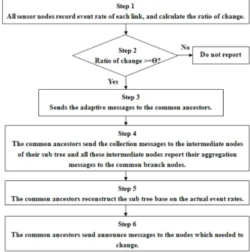
nodes G, H, and I, when the sub tree is changed, as shown in Figure 4(d). The detailed flow chart of the Sub Root MTA procedure is in Figure 5.
Nevertheless, the actual event rates received in the sub root are limited and the sub tree may not need to change after performing the Sub Root Message-Tree Adaptive algorithm. The performance improvement will be limited in Sub Root MTA procedure. Thus, the second layer Sub Root MTA procedure could be introduced to improve the performance. The second layer’s sub root is the second lowest common ancestor of the sensor nodes which perform the MTA procedure. As shown in Figure 4(c), the second layer’s sub root for nodes H and I is node C; the second layer’s sub root for nodes E, F, and J is also node C. Thus, the MTA procedure will be performed under the sub tree whose root is the second layer sub root.
There are some differences between the second layer Sub Root MTA procedure and the Sub Root MTA procedure. In the Sub Root MTA procedure, the adaptive message is sent from the sensor node to the sub root. In the second layer Sub Root MTA procedure, the adaptive message first is sent from the sensor node to the sub root. The sub root will then send the collection message to all intermediate nodes in the sub tree. After receiving the aggregation messages, the sub root will forward the adaptive message to the second layer sub root. The aggregation messages in the sub root will be attached to the adaptive message. Thus, the second layer sub root does not necessarily send the collection message to the sub root. The second layer sub root only needs to send the collection message to the intermediate nodes not in the first layer sub root and not in the sub tree of the first layer sub root.
In the example depicted in Figure 3(c), when nodes A and D receive the adaptive messages sent from nodes E, F, H, I, and J, nodes A and D will send collection messages to nodes G and F, respectively. After receiving the aggregation messages sent from nodes G and F, nodes A and D will forward these adaptive messages with the aggregation messages to node C, respectively. In this case, node A does not need to send any collection messages to any intermediate nodes. The second layer sub root will then announce which nodes needed to change in the new sub tree.
According to the aggregation procedure in the first layer sub root, the number of collection messages will be reduced in the second layer Sub Root MTA procedure. Moreover, third and fourth layer Sub Root Message-Tree Adaptive procedures can also be proposed based on the second layer Sub Root MTA procedure concept and be used to improve the performance.
IV.
EXPERIMENTS AND RESULTS
A. Simulation Setup
A simulator was implemented to evaluate the proposed procedures performance based on the simulation results. The simulations are used to compare the differences between the different layer sub root Message-Tree Adaptive procedures and Message-Tree Adaptive procedure on the sink. The sensing field is 256 × 256, and the number of deployed sensors varied from 100 to 1000, which are randomly deployed in the sensing field.
The sink is in the corner and the object tracking tree is constructed and reconstructed using DAT. The mobility profile is generated based on the city mobility model proposed in [14] and the query rate of each node is randomly assigned. The object made 200,000 moves in each mobility profile to ensure that the resulting mobility profile was statistically significant. To ensure stable results, each simulation ran 100 mobility profiles. The confidence level is 95%, and the confidence intervals were not shown in the figures so that the figures do not become confusing.
In order to show the performance improvement of these MTA procedures, some links will be randomly selected to change its event rates and some nodes will be randomly selected to change its query rates. The range of the threshold value
θ
used was from 5% to 95%. Two performance metrics are considered in this study: the average total cost, and the average adaptation cost. The adaptation cost is used to measure the overhead of the MTA procedure.The MTA procedure overhead can be divided into three parts. The first part is the number of adaptive messages. The adaptive messages should be sent from the sensor nodes that perform the MTA procedure to the sink or sub root. As shown in Figure 4(a), the adaptive messages are sent from nodes E, F, H, I, and J to the sink. Thus, the number of adaptive messages from node I, Report (I) is the hub count between node I and the sink or sub root. The second part is the number of collection and report messages. The collection messages should be sent from the sink or the sub root to the intermediate nodes. The report messages are sent from the intermediate nodes to the sink or the sub root.
As shown in Figure 4(b), nodes A, D, F, and G will receive the collection messages and report the aggregation messages to the sink. Thus, the number of collection and report messages from node I, Collection (I), is two times the hub count between node I and the sink or sub root. The last part is the number of announce message sent from the sink or sub root to the sensor nodes that needed to change after the MTA procedure. As shown in Figure 4(c), nodes G, H, and I will receive the collection messages. Thus, the number of announce message at node I, Announce (I), is the hub count between node I and the sink or sub root. Therefore, the adaptation cost can be defined as follows:
Fig. 6. The Average Total cost (100 links). The improved percentage for all MTA procedures is identical. This is because 100 links are randomly selected to change event rate and in most cases the sub root will be the sink.
TABLEI
THE IMPROVEMENT PERCENTAGE (100 LINKS)
nodes
with L1 SRMTA
with L2 SRMTA
with L3 SRMTA
with L4 SRMTA
with MTA on sink
100 0.935785 0.935785 0.935785 0.935785 0.935785
200 0.940415 0.940415 0.940415 0.940415 0.940415
300 0.934048 0.934048 0.934048 0.934048 0.934048
400 0.933075 0.933075 0.933075 0.933075 0.933075
500 0.933488 0.933488 0.933488 0.933488 0.933488
600 0.934329 0.934329 0.934329 0.934329 0.934329
700 0.932106 0.932106 0.932106 0.932106 0.932106
800 0.930597 0.930597 0.930597 0.930597 0.930597
900 0.927927 0.927927 0.927927 0.927927 0.927927
N
i
)
Announce(i
(i)
Collection
Report(i)
cost
Adaptation
A C
R
S i S
i
S i
∈
+
+
=
∑
∑
∑
∈ ∈
∈
,
(7)where SR represents the set of the sensor node which should
send the adaptive message, SC is the set of sensor node which
receives the collection messages sent from the sink or the sub root, and SA be denoted the set of sensor node that need to
change after the MTA procedure.
B. Results and Discussions
In the following figures and tables, the line denoted by without MTA is the results from the original object tracking tree affected by the changed mobility profile. The line denoted by with MTA on sink is the results from the MTA procedure running on the sink. The line denoted by with L1 SRMTA is the results from the Sub Root Message-Tree Adaptive procedure. The line denoted by with L2 SRMTA is the results from the second layer Sub Root Message-Tree Adaptive procedure, and so on.
In Figures 6 and 7 and Table I, 100 links are randomly selected to change their event rates in the mobility profile, and
θ
is 20%. From Figure 6 and Table I, all of the MTA procedures can significantly improve the total cost for the object tracking tree. Figure 7 shows that the adaptation cost of the MTA on sink is still very large. Due to the aggregation procedure in the first layer sub root, the adaptation cost can be improved using the Sub Root Message-Tree Adaptive procedure. The improved percentage for all MTA procedures is identical. This is because 100 links are randomly selected to change event rate and in most cases the sub root will be the sink.In Figures 8 and 9 and Table II, 10 links are randomly selected to change their event rates in the mobility profile, select 10% nodes to change their query rates, and
θ
is 20%. From Figure 8 and Table 2, all of the MTA procedures can improve the total cost of the object tracking tree. Figure 9 shows that the adaptation cost for the MTA on sink is very large and the adaptation cost can be improved by the Sub Root Message-Tree Adaptive procedure.In Figures 10, 11 and 12, 1 to 100 links are randomly selected to change event rate in the mobility profile. The
θ
still is 20%, and the number of sensor nodes is 1000. From Figures 10 and 12, all of the MTA procedures can significantly improve the total cost for the object tracking tree. When the number of modified links increases, the improvement percentage for all of the MTA procedures becomes identical. Figure 11 also shows that the adaptation cost for the MTA on sink is still very large. Due to the aggregation procedure in the first layer sub root, the adaptation cost can be improved using the Sub Root Message-Tree Adaptive procedure. The adaptation cost slightly increases when the number of modified links increases, and it because that the amount of report message sent from the nodes,whose link is modified, are increased.
Fig. 8. The Average Total cost (10 links with 10% query rate changed) TABLEII
THE IMPROVEMENT PERCENTAGE (10 LINKS WITH 10% QUERY RATE CHANGED)
nodes
with L1 SRMTA
with L2 SRMTA
with L3 SRMTA
with L4 SRMTA
with MTA on sink
100 0.860693 0.845132 0.796272 0.796272 0.795470
200 0.904820 0.894663 0.881479 0.881479 0.881479
300 0.900829 0.896950 0.872664 0.861501 0.861501
400 0.898433 0.884018 0.870090 0.866612 0.866612
500 0.880463 0.866032 0.852764 0.843248 0.843248
600 0.869452 0.857734 0.836514 0.827102 0.825923
700 0.895845 0.875710 0.862641 0.852580 0.852580
800 0.904874 0.889219 0.873564 0.865737 0.865737
900
0.897497 0.883862 0.868181 0.863409 0.863409 7
1000 0.882389 0.864770 0.853024 0.841277 0.841277
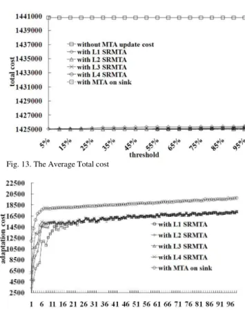
In Figures 13, 14 and 15 and Table III, these results show the performance at different
θ
and different MTA procedures. 20 links are randomly selected to change event rates in the mobility profile. The number of sensor node is 1000. From Figure 13 and Table 3, when theθ
is larger, the average total cost is slightly increased. This is because when theθ
increased, the number of the MTA procedure triggered times decreases and the average total cost will increase. Figure 14 shows that whenθ
is increased the average adaptation cost is decreased. The number of the MTA procedure triggered times decreases whenθ
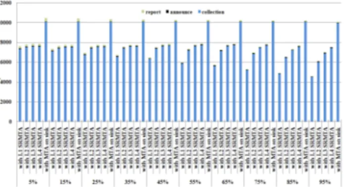
increases.The analysis of the message ratio for the adaptation cost is shown in Figure 15. When
θ
increased, the number of adaptive messages decreases. This is because whenθ
increased, the number of sensor nodes that needed to send adaptive messages decreased, and the number of announcement message does not change too greatly. It is obvious that the most overhead for the adaptation cost comes from the collection and report messages. With the aggregation procedure in the sub root, the adaptation cost can be greatly improved using the Sub Root Message-Tree Adaptiveprocedure
.
Fig. 10. The Average Total cost (1-100 links)
Fig. 14. The Average Adaptation cost
Fig. 13. The Average Total cost
Fig. 11. The Average Adaptation cost (1-100 links) Fig. 9. The Average Total cost (10 links with 10% query rate changed)
From these results, the MTA procedures can significantly improve the total cost when the actual mobility model is very different from the mobility profile, as shown in Figures 10, and 12. Moreover, when the actual mobility model is very different from the mobility profile and
θ
is not larger than 20%, the Sub Root Message-Tree Adaptive procedures can provide good performance in the update and adaptation costs. However, when the actual mobility model is little different from the mobility profile, the system performance has less improvement. Whenθ
is set too high, the system performance also has less improvement.
V. CONCLUSION
Most tree construction algorithms for object tracking proposed are based on a predefined mobility profile and query rates. When the actual object movement behaviors and query rates are very different from the predefined mobility profile, the object tracking tree performance will become worse. To upgrade the object tracking tree, the sink needs to collect the real movement information from the network, and reconstructs the object tracking tree based on the real movement information, but this collection implies in the sink sending very large messages to collect the real movement information from the network, and introduces very large adaptation cost.
In this paper, the Sub Root Message-Tree Adaptive procedures were proposed to provide good total cost with lower adaptation cost. The Sub Root Message-Tree Adaptive procedures collect real movement information from the sub tree, and reconstruct the sub tree based on the real movement information and actual query rates. From the simulation results, our method improves the update and adaptation costs can be improved. From the adaptation cost analysis, most of the adaptation cost overhead is from the collection and report messages. Although the adaptation cost can be improved using the Sub Root MTA procedure, it can still be further improved by future research. For example, from the results shown in Figure 15, the most ratio of adaption cost is the collection cost, and it becauses that the sub root needs to collect the current traffic envieonment. We think that the aggregation mechanism or the multi-sink mechanism [26][27] can be introduced to improve the adaptation cost.
REFERENCES
[1] D. Braginsky and D. Estrin, "Rumor routing algorithm for sensor networks," ACM International Workshop on Wireless Sensor Networks and Applications, 2002.
[2] D. Ganesan, R. Govindan, S. Shenker, and D. Estrin, "Highly resilient, energy efficient multipath routing in wireless sensor networks," ACM Mobile Computer and Communication Review, Vol. 5, No. 4, pp. 11-25, Oct. 2001.
[3] W. R. Heinzelman, A. Chandrakasan, and H. Balakrishnan, "LEACH: Energy-Efficient Communication Protocols for Wireless Microsensor Networks", Hawaiian International Conference on Systems Science, pp. 3005-3014, January 2000.
[4] E. Shih, S.-H. Cho, N. Ickes, R. Min, A. Sinha, A. Wang, and A. Chandrakasan. "Physical layer driven protocol and algorithm design for Fig. 15. The Adaptation cost analysis
TABLEIII THE IMPROVEMENT PERCENTAGE
energy-efficient wireless sensor networks," ACM International Conference on Mobile Computing and Networking, pp. 272-287, 2001. [5] A. Woo and D. E. Culler, "A transmission control scheme for media
access in sensor networks," ACM International Conference on Mobile Computing and Networking, pp. 221-235, 2001.
[6] W. Ye, J. Heidemann, and D. Estrin, "An energy-efficient MAC protocol for wireless sensor networks," IEEE INFOCOM, pp. 1567-1576, 2002. [7] P. Bahl and V. N. Padmanabhan, "RADAR: An in-building RF-based
user location and tracking system," IEEE INFOCOM, pp. 775-784, 2000. [8] N. Bulusu, J. Heidemann, and D. Estrin, "GPS-less low cost outdoor
localization for very small devices," IEEE Personal Communication, Vol. 7, No. 5, pp. 28-34, Oct. 2000.
[9] D. Niculescu and B. Nath, "Ad Hoc Positioning System (APS) using AOA," in Proceedings of IEEE International Conference on Computer Communication (INFOCOM), pp. 1734-1743, March, 2003. [10] F. Aurenhammer, "Voronoi Diagrams - A Survey of a Fundamental
Geometric Data Structure," ACM Computing Surveys, Vol. 23, No. 3, pp. 345-405, September 1991.
[11] Xiang ji Hongyuan Zha Metzner, J.J. Kesidis, G., "Dynamic cluster structure for object detection and tracking in wireless ad-hoc sensor networks", IEEE conference on Communications, Vol. 7, pp. 3807- 3811, June 2004.
[12] DK Guang-yao Jin, Xiao-yi Lu, and Myong-Soon Park, "Dynamic Clustering for Object Tracking in Wireless Sensor Networks", Springer Berlin / Heidelberg, pp. 2000-2009, 2006.
[13] Wen-Chih Peng, Yu-Zen Ko, Wang-Chien Lee, "On Mining Moving Patterns for Object Tracking Sensor Networks", IEEE conference on Mobile Data Management 6, pp. 41- 41, May 2006.
[14] H. T. Kung and D. Vlah "Efficient Location Tracking Using Sensor Networks", IEEE International Conference on wireless communications and networking, 2003.
[15] Chih-Yu Lin, Wen-Chih Peng, and Yu-Chee Tseng, "Efficient In-Network Moving Object Tracking in Wireless Sensor Networks", IEEE Transactions on Mobile Computing, Vol. 5, pp. 1044-1056, Aug. 2006.
[16] Chih-Yu Lin, Yu-Chee Tseng, Wen-Chih Peng, "Message-Efficient In-Network Location Management in a Multi-sink Wireless Sensor Network", IEEE International Conference on Sensor Networks, Ubiquitous, and Trustworthy Computing, pp: 496 - 505, 2006. [17] Hua-Wen Tsai, Chih-Ping Chu, Tzung-Shi Chen, "Mobile Object
Tracking in Wireless Sensor Networks", Computer Communications, Vol. 30, No. 8, pp. 1811-1825, June 2007.
[18] Vincent S. Tseng and Kawuu W. Lin, "Energy Efficient Strategies for Object Tracking in Sensor Networks: A Data Mining Approach", Journal of Systems and Software, Vol. 80, No. 10, pp. 1678-1698, October 2007. [19] Bing-Hong Liu, Wei-Chieh Ke, Chin-Hsien Tsai, and Ming-Jer Tsai,
"Constructing a Message-pruning tree with minimum Cost for Tracking moving objects in wireless sensor networks Is NP-Complete and an enhanced data aggregation structure", IEEE Transactions on Computers, Vol. 57, pp. 849-863, June 2008.
[20] Min-Xiou Chen, and Yin-Din Wang, "An Efficient Location Tracking Struct ure for Wireless Sensor Networks", Computer Communications, Vol. 32, No. 8. 1495-1504, Aug. 2009.
[21] Li-Hsing Yen, and Chia-Cheng Yang, "Mobility Profiling Using Markov Chains for Tree-Based Object Tracking in Wireless Sensor Networks", IEEE International Conference on Sensor Networks, Ubiquitous, and Trustworthy Computing, Vol. 2, pp. 220 - 225, 2006.
[22] Min-Xiou Chen, Che-Chen Hu and Wen-Yen Weng, "Dynamic Object Tracking Tree in Wireless Sensor Network", EURASIP Journal on Wireless Communications and Networking, special issue for Theoretical and Algorithmic Foundations of Wireless Ad Hoc and Sensor Networks, 2010. doi: 10.1155/2010/386319
[23] Xuewen Wu, Guan Huang, Dunye Tang and Xinhong Qian, "A Novel Adaptive Target Tracking Algorithm in Wireless Sensor Networks", Communications in Computer and Information Science, 2011, Volume 135, 477-486, DOI: 10.1007/978-3-642-18134-4_76.
[24] E.P. Freitas, B. Bösch, R.S. Allgayer, L. Steinfeld, F.R. Wagner, L. Carro, C.E. Pereira, and T. Larsson, "Mobile Agents Model and Performance Analysis of a Wireless Sensor Network Target Tracking Application", Proceedings of the 11th international conference and 4th international conference on Smart spaces and next generation wired/wireless networking, 274-286, 2011.
[25] Y. Xu, and H.Qi, "Mobile agent migration modeling and design for target tracking in wireless sensor networks", Ad Hoc Networks, No. 6, Vol. 1, 1-16, January, 2008.
[26] D Liu, J Zhang, “A multi-sink and multi-object tracking strategy for wireless sensor networks”, Proceedings of the 2011 International Conference on Electrical and Control Engineering (ICECE), 4273-4276, 2011.