Modeling the effects of size on patch dynamics of an inert tracer

(1)

OSD

6, 1735–1756, 2009

Modeling patch dynamics of an inert

tracer

P. Xiu and F. Chai

Title Page

Abstract Introduction

Conclusions References

Tables Figures

◭ ◮

Back Close

Full Screen / Esc

Printer-friendly Version

Interactive Discussion

Ocean Sci. Discuss., 6, 1735–1756, 2009 www.ocean-sci-discuss.net/6/1735/2009/

Ocean Science Discussions

Papers published inOcean Science Discussionsare under open-access review for the journalOcean Science

Modeling the e

_ff

ects of size on patch

dynamics of an inert tracer

P. Xiu and F. Chai

School of Marine Sciences, University of Maine, Orono, Maine, USA

Received: 21 July 2009 – Accepted: 6 August 2009 – Published: 14 August 2009

Correspondence to: P. Xiu (pengxiucn@gmail.com)

(2)

OSD

6, 1735–1756, 2009

tracer

P. Xiu and F. Chai

Title Page

Tables Figures

◭ ◮

Back Close

Full Screen / Esc

Interactive Discussion Abstract

Mesoscale iron enrichment experiments have revealed that additional iron affects the phytoplankton productivity and carbon cycle. However, the role of initial size of fertilized patch in determining the patch evolution is poorly quantified due to the limited time of research vessels at sea. Using a three-dimensional ocean circulation model, we

5

simulated different sizes of inert tracer patches that were only regulated by physical circulation and diffusion. Model results showed that during the first few days since release of inert tracer, the calculated dilution rate was found to be a linear function with time, which was sensitive to the initial patch size with steeper slope for smaller size patch. After the initial phase of rapid decay, the relationship between dilution rate

10

and time became an exponential function, which was also size dependent. Therefore, larger initial size patches can usually last longer and ultimately affect biogeochemical processes much stronger than smaller patches.

1 Introduction

Since 1993, Martin’s iron hypothesis that iron availability limits ocean productivity

(Mar-15

tin, 1990), has been confirmed by 12 mesoscale iron enrichment experiments in dif-ferent high nitrate-low chlorophyll (HNLC) regions, such as the equatorial Pacific, the Southern Ocean, the subarctic Pacific, etc. (Coale et al., 1996; Boyd et al., 2000; Tsuda et al., 2003; Coale et al., 2004; de Baar et al., 2005). These experiments also revealed that iron could further influence carbon cycle inside the iron patch, including

20

air-sea CO2flux and vertical carbon export (Boyd et al., 2007). However, extrapolation

of these results to regional and long-term impact of additional iron on biogeochemical processes is still unclear. This is mainly due to the logistic constrains that the research vessels can only remain within the iron patch for 30 to 40 days, which is usually not long enough to observe the complete impact of iron and the entire iron patch

disper-25

(3)

OSD

6, 1735–1756, 2009

tracer

P. Xiu and F. Chai

Title Page

Tables Figures

◭ ◮

Back Close

Full Screen / Esc

past 12 iron enrichment experiments, while different initial sizes of the iron patch were created (e.g. 64 km2 for IronEx-1; 50 km2 for SOIREE; 225 km2 for Sofex), the impact of iron on phytoplankton bloom and carbon cycling were not assessed due to diff er-ent sizes of iron patches. The different locations of these iron enrichment experiments make it very di_fficult to address how di_fferent physical processes a_ffect movement and

5

dilution of an iron patch.

The movement and reshaping of the fertilized patch are controlled primarily by the circulation and di_ffusion processes, and the chemical and biological processes inside the patch will follow the movement of the patch accordingly. Inside the iron patch, the nutrients and phytoplankton bloom dynamics and carbon cycle have been addressed

10

using both field observations and the modeling approach (Gnanadesikan et al., 2003; de Baar et al., 2005; Fujii et al., 2005; Chai et al., 2007; Boyd et al., 2007). For the phys-ical processes controlling a surface patch, there are three stages of dispersion (Garrett, 1983). The first stage is a linear growth; after reaching a size where the mesoscale strain field begins to advect the patch into long streaks, the patch enters the second

15

stage with an exponential growth; after that, the third stage is in which surface area begins to increase linearly again. For all of the iron enrichment experiments, the iron patches usually start with a scale of∼1000 m. Although most of the observed patches

are at their second stage (Abraham et al., 2000; Ledwell et al., 1998), sometimes the second and third stage of the patch can be observed if only the experiment lasts long

20

enough (Sundermeyer and Price, 1998). These in-situ observations mainly focused on the expanding period of a patch, however, the detailed patch dynamics of inert tracer and long-term variations are still not well understood. Plankton dynamics and carbon cycle are influenced both in the expanding and contracting periods of an iron patch, thus it is important to investigate how physical processes affect patch movement and

25

dispersion regarding to long-term impact of iron fertilization experiments.

(4)

OSD

6, 1735–1756, 2009

tracer

P. Xiu and F. Chai

Title Page

Tables Figures

◭ ◮

Back Close

Full Screen / Esc

carbon cycle (Fujii et al., 2005; Jiang and Chai, 2004; Jin et al., 2008). This study examines how physical processes affect surface patch dynamics and focuses on the role of the initial patch size in controlling patch dispersion. The modeled information is useful for designing and conducting large-scale iron enrichment experiments in the future.

5

2 Model description and experimental design

The model used in this study is a three-dimensional ocean circulation model, Regional Ocean Modeling System (ROMS), which represents an evolution in the family of terrain-following vertical coordinate models. ROMS solves the hydrostatic, primitive equations with horizontal curvilinear coordinates. Wang and Chao (2004) have configured the

10

ROMS circulation model for the Pacific Ocean (45◦_{S to 65}◦_{N, 99}◦_{E to 70}◦_{W) at 50 km}

resolution, with realistic geometry and topography. For this biogeochemical modeling study, we followed the approach of Wang and Chao (2004) for setting up the circulation model, but increase the horizontal resolution to 12.5 km for the entire model domain. There are 30 levels in the vertical. Near the two closed northern and southern walls,

15

a sponge layer with a region of 5◦ _{from the walls is applied for temperature, salinity,}

and nutrients. The treatment of the sponge layer consists of a decay term κ(T*–T) in the temperature equation κ(S*–S) for salinity equation, κ(N*–N) for nutrient and carbon equations), which restores the modeled variables to the observed tempera-ture T* (salinity S*, nutrients N*) field at the two closed walls. The value of κ varies

20

smoothly from 1/30 day−1 _{at the walls to zero at 5 degrees away from them. Liu and}

Chai (2009) and Chai et al. (in press) coupled the biogeochemical Carbon, Silicate, Nitrogen Ecosystem (CoSiNE) model (Chai et al., 2002) with the Pacific ROMS to study the seasonal and interannual variability of phytoplankton productivity and carbon fluxes.

25

(5)

OSD

6, 1735–1756, 2009

tracer

P. Xiu and F. Chai

Title Page

Tables Figures

◭ ◮

Back Close

Full Screen / Esc

the Pacific ROMS-CoSINE model has been forced with the climatological NCEP/NCAR reanalysis of air-sea fluxes (Kalnay et al., 1996) calculated using the bulk formula for several decades in order to reach quasi-equilibrium. The ROMS model is then forced with daily air-sea fluxes of heat and freshwater derived from the NCEP/NCAR reanaly-sis (Kalnay et al., 1996). The blended daily sea winds with resolution of 0.25◦_(Zhang 5

et al., 2006) is used to calculate the surface wind stress based on the bulk formula of Large and Pond’s (1982). The heat flux is derived from the short- and long-wave radiations, sensible and latent heat fluxes that are calculated using the bulk formula with prescribed air temperature and relative humidity. The fresh-water flux is derived from the prescribed precipitation and the evaporation converted from the latent heat

10

release. River discharges are not included in the model configuration.

To investigate patch dynamics, an inert tracer (IT) is introduced, which is controlled only by circulation and diffusion. The behavior of this IT is very similar to the SF6 tracer used during the iron fertilization experiments (Law et al., 1998; Boyd et al., 2004; Law et al., 2006). Our model experiments include six different initial sizes of IT patch

15

(Table 1) in the eastern equatorial Pacific Ocean (3◦_{S, 90}◦_{W), close to the locations}

of the IronEx I and IronEx II experiments. For each model experiment, IT tracer was continuously added into the upper 30 m during 14 days starting from 7 January 2004. After 14 days injection of IT, we normalized the IT concentration with respect to IT0

(the highest concentration of IT at day 14) first, then defined the IT patch as where the

20

normalized IT concentration (denoted as the IT concentration hereafter) is higher than 0.1 (10% versus 1/e used by Law et al., 2006). By doing so, this allows us to compare results among di_fferent sizes of the IT patch. In order to estimate the movement and reshaping of the IT patch during each time step, Gaussian ellipse fitting technique was applied to the modeled surface IT concentration. This is because that at scales greater

25

(6)

OSD

6, 1735–1756, 2009

tracer

P. Xiu and F. Chai

Title Page

Tables Figures

◭ ◮

Back Close

Full Screen / Esc

well described by a Gaussian ellipse as (e.g. Abraham et al., 2000; Law et al., 2006)

C=( N 2πσxσy

) exp(−

(x2/σ_x2+y2/σ_y2)

2 ) (1)

whereC is the IT concentration,N is the total amount of tracer within the patch and σx(t), σy(t) are the standard deviations of the distribution in the x and y directions,

respectively. After an initial adjustment, strain and dilution rates of the surface IT patch

5

were then calculated from the changes in the dimensions of the Gaussian ellipse, by using nonlinear fitting procedure (see methods below, Abraham et al., 2000).

3 Results and discussion

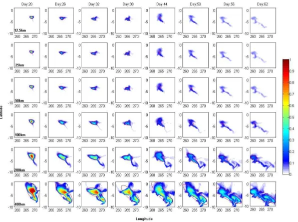
The modeled surface patch follows a similar pattern regardless of the initial patch size, generally moves cyclonically with its center moving toward the northwest direction

dur-10

ing the first 60 days of the simulation (Fig. 1). The lateral dispersion is largely de-termined by stirring associated with eddies (Garrett, 1983; Abraham et al., 2000), which changes from an initial square area to a narrow filament. For example, the initial 12.5×12.5 km patch by day 38 evolves into a filament with a length of 225.2 km,

a width of 126.3 km and the resultant eccentricity of 0.83; at the same time, the initial

15

400×400 km patch turns into a narrow filament with a length of 1865.7 km, a width of

375.4 km and a much higher eccentricity of 0.98. During the modeled experiments, smaller patches tend to have lower IT concentration and disappear much faster than larger patches (Table 1). The “disappearing day” in Table 1 is the day when IT concen-tration everywhere within the model domain becomes lower than 0.1, though at some

20

days Gaussian ellipse fit could not be applied mainly due to the patch being too small. 12.5×12.5 km patch starts with a surface area of 17969 km2, reaches its maximum of

(7)

OSD

6, 1735–1756, 2009

tracer

P. Xiu and F. Chai

Title Page

Tables Figures

◭ ◮

Back Close

Full Screen / Esc

52.6% larger than first day volume, and disappears at day 56. For surface area, the ra-tio of maximum to the first day value is 1.67 for large patches (mean value of 100×100,

200×200 and 400×400 patches), which is higher than 1.44 for small patches (mean

value of 12.5×12.5, 25×25 and 50×50 patches). While for total volume, the ratio is

1.40 for large patches, which is a little lower than 1.50 for small patches.

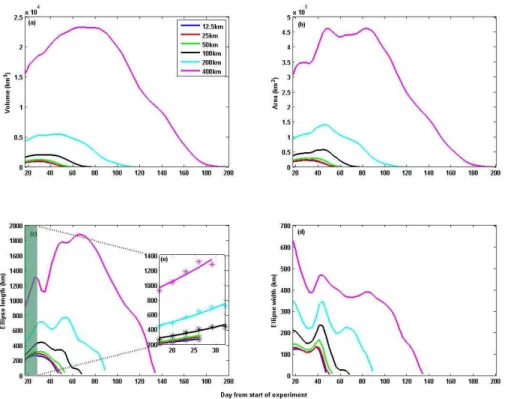
5

For patches of all sizes, both the surface area and total volume of the patch generally increases with time at first due to the high IT concentration inside the patch. Then, after reaching its peak, it starts to decrease gradually until it disappears (Fig. 2a, b). This trend is hard to obtain from in-situ measurements and most of the field experiments only focus on the expanding period of the patch due to the limited time of observation

10

(Timothy et al., 2006; Boyd et al., 2004). Comparison among di_fferent initial patch sizes indicates that large patches have longer peak time than small patches. Peak time is defined as the day when the value of the surface area or total volume reaches its maximum. Surface area peak time for both the 12.5×12.5 km and the 25×25 km

patch is about 23 days after the start of the experiment, while for larger patches, the

15

patch could continue expanding until more than 40 days before reaching the peak of its surface area. Disappear day is the day when the surface concentration falls below the preset limit, which can be used to describe the entire life history of the patch. Both the 12.5×12.5 km and the 25×25 km patch can last 56 days, the 200×200 km patch

per-sists for about 113 days, which is twice the duration of the12.5×12.5 km patch, while the 20

400×400 km patch lasts three times longer (194 days) than the 12.5×12.5 km patch.

The disappear day for surface area is the same as that for total volume, indicating the patch mostly exists in the upper water column that is consistent with iron fertilization experiments.

Previous studies showed that, in the first few days during the patch expansion, length

25

(8)

OSD

6, 1735–1756, 2009

tracer

P. Xiu and F. Chai

Title Page

Tables Figures

◭ ◮

Back Close

Full Screen / Esc

described as the second stage of the tracer dispersion suggested by Garrett (1983). In this study, the strain rate (γ) is calculated by applying a nonlinear fitting procedure to modeled σ_x(t) and time (t). During the first 32 days in this modeling study, a ro-bust exponential function is found to fit well to the length data (Fig. 2c). Though the magnitude of ellipse length varies in response to the different initial patch sizes, the

5

calculated strain rates are almost the same for all patches (γ=0.03 day−1_{). This strain}

rate is a little lower than the previous values of 0.07 day−1_{reported for the SOIREE}

iron fertilization (Abraham et al., 2000) and 0.08 day−1 _{estimated for the sub-Arctic}

Pacific fertilization experiment (Law et al., 2006), indicating different dilution rates in different areas. The difference among these results might be due to both the diff

er-10

ent observational time lengths and the di_fferent physical conditions related to the high spatial and temporal variability of strain in ocean currents (Sundermeyer and Price, 1998; Law et al., 2006). Law et al. (2006) suggested that different strain rate might be caused by di_fferent initial release area during the experiments, however, the strain rate is relatively stable over different initial area patches and we do not see any clear

15

relationship between strain rate and initial area in this study. While note that, our re-sults do not include biological activities, which might a_ffect patch dynamics significantly. Ellipse width, however, decreases within this period of time, which is attributed to the stronger convergent strain rather than the small scale diffusion or mixing (Sundermeyer and Price, 1998). As a result, increasing length and decreasing width leads to an

in-20

creasingly longer and narrower filament (Fig. 2c, d). After day 32, ellipse length starts to decrease and width starts to increase for about one week. It is likely caused by the unique, local physical conditions because such fluctuation has neither been ob-served nor modeled before. For the entire life history of the IT patch, variation of length derived from the fitted Gaussian ellipse looks much like a second-order polynomial

25

(9)

OSD

6, 1735–1756, 2009

tracer

P. Xiu and F. Chai

Title Page

Tables Figures

◭ ◮

Back Close

Full Screen / Esc

400×400 km patch), which means the width remains relatively more constant than the

length. For in-situ experiments, previous studies often use either linear or exponen-tial functions to model observed variations of surface patch. From the model results, however, it is unclear whether the observed surface patch area is an exponential (Law et al., 2006), exponential and linear (Sundermeyer and Price, 1998), or polynomial

5

function with time, since that depends on both the observational period and the local physical conditions.

To further investigate how di_fferent size patches disperse, we define and calculate the dilution rate (r) of the surface area and total volume as

r = A(t+ ∆t)−A(t)

A(t)∗∆t

(2)

10

whereAis the area or volume, t is time, and _∆t is the time interval (Abraham et al., 2000; de Baar et al., 2005). The unit for the dilution rate r is day−1_{. Overall, two}

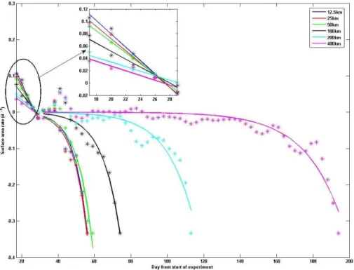
stages are found for both the surface area and total volume (Figs. 3 and 4). In the first stage, the calculated rate decreases linearly with time for about 30 days, which can be expressed as

15

r =a1t+b1 (3)

wherea1andb1are the regression coefficients,r denotes the dilution rate (day− 1

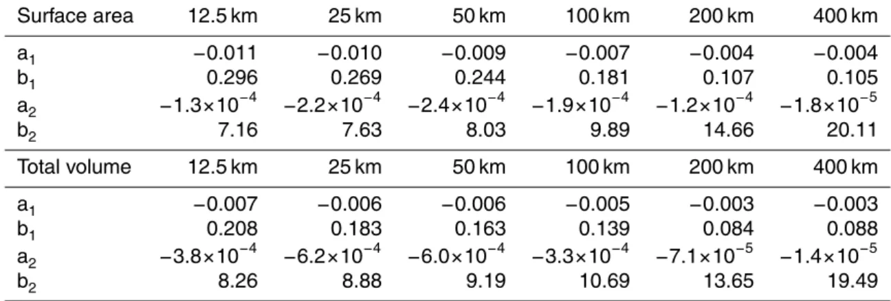
) and tis the time. Linear regression analysis shows that smaller patch tends to have steeper slope (Table 2), which results in less stable expanding relative to larger patch. After 30 days when dilution rate reaches zero, the patch enters its second stage. Smaller

20

patches, such as the 12.5×12.5 km and the 25×25 km ones, start to decrease much

earlier than larger patches (400×400 km). Larger patches can maintain their zero

di-lution rate for a very long time (e.g. over 100 days for the 400×400 km patch). For the

entire second stage, an exponential function is used here to regress the rate data:

r =a2exp(t/b2) (4)

(10)

OSD

6, 1735–1756, 2009

tracer

P. Xiu and F. Chai

Title Page

Tables Figures

◭ ◮

Back Close

Full Screen / Esc

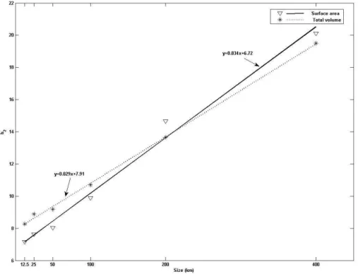
wherea2and b2are the regression coefficients. In this equation, the coefficientb2is

the one that controls the duration time in which the patch could maintain its zero dilution rate. The higher the value ofb2, the longer the duration time. Furthermore, the value of

b2is also shown to be size-dependent, which can be estimated well by a linear function

of the initial size both for the surface area and total volume data (Fig. 5), implying that

5

a larger initial patch has stronger ability to maintain despite the destruction of physical circulation and diffusion.

We also conducted the same set of experiments for 2005 at the same spatial lo-cation. Different from 2004, the peak time of the surface area for the 400×400 patch

is 65 days, which is longer than year 2004 (44 days). Yet, the 12.5×12.5, 25×25, 10

50×50, 100×100 and 200×200 patches are the same as the year 2004, i.e. 23 days.

On the other hand, the disappearing day for 2005 is much longer than for 2004. For example, in the case of the 12.5×12.5 patch, the disappearing day is 86 days for 2005

and 56 days for 2004; for the 200×200 patch it is 155 days for 2005 and 113 days for

2004. It is difficult to generalize the development of different stages with time as

de-15

scribed by Garrett (1983), especially using the patch measurements alone. However, the high-resolution physical models can provide detailed information about evaluation of patch dynamics, especially for different regions and/or year-to-year variations. Two similar stages of linear and exponential relationship for the dilution rate are also found for 2005, which are similar to 2004 in terms of timing in switching between these two

20

stages. The linear relationship exists during the first 40 days, still with steeper slope for smaller initial size patch. Theb2 values from exponential regression are also found to

be correlated linearly with the initial patch size (see Fig. 5 for the 2004 case), though the magnitudes are slightly different from the 2004 case. The dilution rates during the first stage are mostly higher than zero, indicating the patch is in its expanding phase.

25

(11)

en-OSD

6, 1735–1756, 2009

tracer

P. Xiu and F. Chai

Title Page

Tables Figures

◭ ◮

Back Close

Full Screen / Esc

vironment, such as surface wind, current, and diffusion effect. These results again show that local physical conditions are an important factor a_ffecting patch dispersal and movement.

While there is little discussion remaining over whether iron limits production in HNLC regions, there is still significant debate on whether these results could be

extrapo-5

lated to larger spatial scale and long-term effects (Boyd et al., 2007). Buesseler et al. (2008) argued that ecological impacts of iron fertilization and CO2 mitigation are

scale-dependent, and they also recommended the use of high-resolution models to assess downstream effects beyond the study area and observation period. Chai et al. (2007) suggested that for the larger patch experiments, amount of phytoplankton

10

biomass increase stimulated by iron is much greater than the smaller patch, which al-lows more phytoplankton being retained within the patch. Our results show that the patch dilution effect is more pronounced in the smaller patches than the larger ones. In addition, the larger patches tend to have more nutrients than smaller ones, which could continue to fuel the phytoplankton bloom. As a result, with the same duration

15

period of iron fertilization, the larger patches could produce broader spatial extent and longer lasting phytoplankton bloom. Bowie et al. (2001) identified that patch dilution is a major pathway for the decline of added dissolved iron during their experiments. Law et al. (2006) demonstrated that dilution rate has potential impact on the onset of phyto-plankton bloom termination and export. The model results from this study indicate that

20

physical dilution rate is not a constant but varies with time. It is largely related to the initial patch size. We speculate that initial patch size can affect patch dilution directly, which has impact on the fate of added iron in the iron enrichment experiments, could further influence the biogeochemical dynamics inside the patch.

In summary, this study shows that in order to study long-term effects of iron

fertiliza-25

(12)

OSD

6, 1735–1756, 2009

tracer

P. Xiu and F. Chai

Title Page

Tables Figures

◭ ◮

Back Close

Full Screen / Esc

sensitive to the initial size. The total volume of materials injected and local physical con-ditions also play a role in determining the evaluation of patch dynamics and its impact on ecosystems and carbon cycling. For ocean iron fertilization experiments, besides the size of initial iron patch and total iron injected, repeatedly adding iron to the same patch of water can also maintain high iron concentration, therefore creating long

last-5

ing effects. Modeled results provide important information that can guide large-scale iron fertilization experiments. Detailed field measurements and long-term monitoring, including ecosystem responses to iron fertilization and the fate of fixed carbon, would improve modeling capability and allow us to assess the efficacy of sequestrating atmo-spheric CO2to the deep sea.

10

Acknowledgements. We thank Yi Chao at JPL/NASA for sharing the ROMS circulation model configuration for the Pacific Ocean, and Lei Shi at the University of Maine for designing and setting up the tracer experiments.

References

Abraham, E. R., Law, C. S., Boyd, P. W., Lavender, S. J., Maldonado, M. T., and Bowie, A. R.:

15

Importance of stirring in the development of an iron-fertilized phytoplankton bloom, Nature, 407, 727–730, 2000.

Bowie, A. R., Maldonado, M. T., Frew, R. D., Croot, P. L., Achterberg, E. P., Mantoura, R. F. C., Worsfold, P. J., Law, C. S., and Boyd, P. W.: The fate of added iron during a mesoscale fertilisation experiment in the Southern Ocean, Deep-Sea Res. II, 48, 2703–2743, 2001.

20

Boyd, P. W., Watson, A. J., Law, C. S., Abraham, E. R., Trull, T., Murdoch, R., Bakker, D. C. E., Bowie, A. R., Buesseler, K. O., Chang, H., Charette, M., Croot, P., Downing, K., Frew, R., Gall, M., Hadfield, M., Hall, J., Harvey, M., Jameson, G., LaRoche, J., Liddicoat, M., Ling, R., Maldonado, M. T., McKay, R. M., Nobber, S., Pickmere, S., Pridmore, R., Rintoul, S., Safi, K., Sutton, P., Strzepek, R., Tanneberger, K., Turner, S., Waite, A., and Zeldis, J.: Phytoplankton

25

bloom upon mesoscale iron fertilization of polar Southern Ocean water, Nature, 407, 695– 702, 2000.

(13)

Barwell-OSD

6, 1735–1756, 2009

tracer

P. Xiu and F. Chai

Title Page

Tables Figures

◭ ◮

Back Close

Full Screen / Esc

Clarke, J., Crawford, W., Crawford, D., Hale, M., Harada, K., Johnson, K., Kiyosawa, H., Kudo, I., Marchetti, A., Miller, W., Needoba, J., Nishioka, J., Ogawa, H., Page, J., Robert, M., Saito, H., Sastri, A., Sherry, N., Soutar, T., Sutherland, N., Taira, Y., Whitney, F., Wong, S. K. E., and Yoshimura, T.: The decline and fate of an iron-induced subarctic phytoplankton bloom, Nature, 428, 549–553, 2004.

5

Boyd, P. W., Jickells, T., Law, C. S., Blain, S., Boyle, E. A., Buesseler, K. O., Coale, K. H., Cullen, J. J., de Baar, H. J. W., Follows, M., Harvey, M., Lancelot, C., Levasseur, M., Owens, N. P. J., Pollard, R., Rivikin, R. B., Sarmiento, J., Schoemann, V., Smetacek, V., Takeda, S., Tsuda, A., Turner, S., and Watson, A. J.: Mesoscale iron enrichment experiments 1993– 2005: Synthesis and future directions, Science, 315, 612–617, 2007.

10

Buesseler, K. O. and Boyd, P. W.: Will ocean fertilization work? Nature, 300, 67–68, 2003. Buesseler, K. O., Doney, S. C., Karl, D. M., Boyd, P. W., Caldeira, K., Chai, F., Coale, K. H., de

Baar, H. J. W., Falkowski, P. G., Johnson, K. S., Lampitt, R. S., Michaels, A. F., Naqvi, S. W. A., Smetacek, V., Takeda, S., and Watson, A. J.: Ocean iron fertilization-Moving forward in a sea of uncertainty, Science, 319, p. 162, 2008.

15

Chai, F., Dugdale, R. C., Peng, T. H., Wilkerson, F. P., and Barber, R. T.: One dimensional ecosystem model of the Equatorial Pacific upwelling system, Part I: Model development and silicon and nitrogen cycle, Deep-Sea Res. II, 49, 2713–2745, 2002.

Chai, F., Jiang, M., Chao, Y., Dugdale, R. C., Chavez, F., and Barber, R. T.: Modeling responses of diatom productivity and biogenic silica export to iron enrichment in the equatorial Pacific

20

Ocean, Global Biogeochem. Cycles, 21, GB3S90, doi:10.1029/2006GB002804, 2007. Chai, F., Liu, G., Xue, H., Shi, L., Chao, Y., Tseng, C. M., Chou, W. C., and Liu, K. K.: Seasonal

and interannual variability of carbon cycle in South China Sea: a three dimensional physical-biogeochemical modeling study, J. Oceanogr., in press, 2009.

Coale, K. H., Johnson, K. S., Fitzwater, S. E., Gordon, R. M., Tanner, S., Chavez, F. P., Ferioli,

25

L., Sakamoto, C., Rogers, P., Millero, F., Steinberg, P., Nightingale, P., Cooper, D., Cochlan, W. P., Landry, M. R., Constantinou, J., Rollwagen, G., Trasvina, A., and Kudela, R.: A mas-sive phytoplankton bloom induced by an ecosystem-scale iron fertilisation experiment in the equatorial Pacific Ocean, Nature, 383, 495–501, 1996.

Coale, K. H., Johnson, K. S., Chavez, F. P., Buesseler, K. O., Barber, R. T., Brzezinski, M. A.,

30

(14)

OSD

6, 1735–1756, 2009

tracer

P. Xiu and F. Chai

Title Page

Tables Figures

◭ ◮

Back Close

Full Screen / Esc

R., Demarest, M., Hiscock, W. T., Sullivan, K. F., Tanner, S. J., Gordon, R. M., Hunter, C. N., Elrod, V. A., Fitzwater, S. E., Jones, J. L., Tozzi, S., Koblizek, M., Roberts, A. E., Herndon, J., Brewster, J., Ladizinsky, N., Smith, G., Cooper, D., Timothy, D., Brown, S. L., Selph, K. E., Sheridan, C. C., Twining, B. S., and Johnson, Z. I.: Southern Ocean iron enrichment experiment: carbon cycling in high- and low-Si water, Science, 304, 408–414, 2004.

5

de Baar, H. J. W., Boyd, P. W., Coale, K. H., Landry, M. R., Tsuda, A., Assmy, P., Bakker, D. C. E., Bozec, Y., Barber, R. T., Brzeinski, M. A., Buesseler, K. O., Boy ´e, M., Croot, P. L., Gervais, F., Gorbunov, M. Y., Harrison, P. J., Hiscock, W. T., Laan, P., Lancelot, C., Law., C. S., Levasseur, M., Marchetti, A., Millero, F. J., Nishioka, J., Nojiri, Y., van Oijen, T., Riebesell, U., Rijkenberg, M. J. A., Saito, H., Takeda, S., Timmermans, K. R., Veldhuis, M. J. W., Waite,

10

A. M., and Wong, C. S.: Synthesis of iron fertilization experiments: From the iron age in the age of enlightenment, J. Grophys. Res., 110, C09S16, doi:10.1029/2004JC002601, 2005. Fujii, M., Yoshie, N., Yamanka, Y., and Chai, F.: Simulated biogeochemical responses to iron

enrichments in three high nutrient, low chlorophyll (HNLC) regions, Prog. Oceanogr., 64, 307–324, 2005.

15

Garrett, C.: On the initial streakiness of a dispersing tracer in two- and three-dimensional tur-bulence, Dyn. Atmos. Oceans., 7, 265–277, 1983.

Gnanadesikan, A., Sarmiento, J. L., and Slater, R. D.: Effects of patchy ocean fertilization on atmospheric carbon dioxide and biological productivity, Global Biogeochem. Cycles., 17, 1050, doi:10.1029/2002GB001940, 2003.

20

Jiang, M. and Chai, F.: Iron and silicate regulation on new and export production in the equatorial Pacific: A physical-biological model study, Geophys. Res. Lett., 31, doi:10.1029/2003GL018598, 2004.

Jin, X., Gruber, N., Frenzel, H., Doney, S. C., and McWilliams, J. C.: The impact on atmospheric CO₂of iron fertilization induced changes in the ocean’s biological pump, Biogeosciences., 5,

25

385–406, 2008.

Kalnay, E., Kanamitsu, M., Kistler, R., Collins, W., Deaven, D., Gandin, L., Iredell, M., Saha, S., White, G., Woollen, J., Zhu, Y., Chelliah, M., Ebisuzaki, W., Higgins, W., Janowiak, J., Mo, K. C., Ropelewski, C., Wang, J., Jenne, R., and Joseph, D.: The NCEP/NCAR 40-year reanalysis project, Bull. Am. Meteor. Soc., 77, 437–471, 1996.

30

Large, W. G. and Pond, S.: Sensible and latent heat flux measurements over the ocean, J. Phys. Oceanogr., 12, 464–482, 1982.

(15)

OSD

6, 1735–1756, 2009

tracer

P. Xiu and F. Chai

Title Page

Tables Figures

◭ ◮

Back Close

Full Screen / Esc

biogeochemical and physical processes in an open-ocean iron fertilisation experiment, Deep Sea Res. II, 45, 977–994, 1998.

Law, C. S., Crawford, W. R., Smith, M. J., Boyd, P. W., Wong, C. S., Nojiri, Y., Robert, M., Abraham, E. R., Johnson, W.K., Forsland, V., and Arychuk, M.: Patch evolution and the biogeochemical impact of entrainment during an iron fertilisation experiment in the sub-Arctic

5

Pacific, Deep Sea Res. II, 53, 2012–2033, 2006.

Ledwell, J. R., Watson, A. J., and Law, C. S.: Mixing of a tracer in the pycnocline, J. Grophys. Res., 103, 21499–21529, 1998.

Liu, G. and Chai, F.: Seasonal and interannual variability of primary and export production in the South China Sea: a three-dimensional physical–biogeochemical model study, ICES J.

10

Marine Syst., 66, 420–431, 2009.

Martin, J. H.: Glacial-interglacial CO₂change: the iron hypothesis, Paleoceanography., 5, 1–13, 1990.

Sundermeyer, M. A. and Price, J. F.: Lateral mixing and the north Atlantic tracer release exper-iment: observations and numerical simulations of Lagrangian particles and a passive tracer,

15

J. Grophys. Res., 103, 21481–21497, 1998.

Timonthy, D. A., Wong, C. S., Nojiri, Y., Ianson, D. C., and Whitney, F. A.: The effects of patch expansion on budgets of C,N and Si for the Subarctic Ecosystem Response to Iron Enrichment Study (SERIES), Deep Sea Res. II, 53, 2034–2052, 2006.

Tsuda, A., Takeda, S., Saito, H., Nishioka, J., Nojiri, Y., Kudo, I., Kiyosawa, H., Shiomoto, A.,

20

Imai, K., Ono, T., Shimamoto, A., Tsumune, D., Yoshimura, T., Aono, T., Hinuma, A., Kinu-gasa, M., Suzuki, K., Sohrin, Y., Noiri, Y., Tani, H., Deguchi, Y., Tsurushima, N., Ogawa, H., Fukami, K., Kuma, K., and Saino, T.: A mesoscale iron enrichment in the western subarctic Pacific induces a large centric diatom bloom, Science, 300, 958–961, 2003.

Wang, X. and Chao, Y.: Simulated sea surface salinity variability in the tropical Pacific,

Geo-25

phys. Res. Lett., 31, L02302, doi:10.1029/2003GLD18146, 2004.

(16)

OSD

6, 1735–1756, 2009

tracer

P. Xiu and F. Chai

Title Page

Tables Figures

◭ ◮

Back Close

Full Screen / Esc

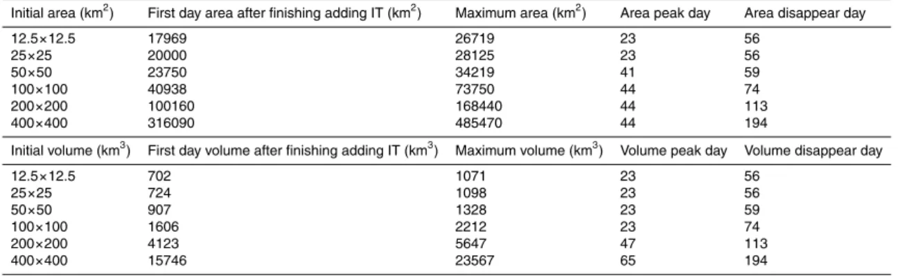
Table 1. Modeled results for the six experiments conducted in this study (Maximum area is

the largest area each patch can occupy, Area peak day is the day at which the patch reach its maximum area, and the Area disappear day is the day which IT concentration becomes lower than 0.1 within that region).

Initial area (km2) First day area after finishing adding IT (km2) Maximum area (km2) Area peak day Area disappear day

12.5×12.5 17969 26719 23 56

25×25 20000 28125 23 56

50×50 23750 34219 41 59

100×100 40938 73750 44 74

200×200 100160 168440 44 113

400×400 316090 485470 44 194

Initial volume (km3) First day volume after finishing adding IT (km3) Maximum volume (km3) Volume peak day Volume disappear day

12.5×12.5 702 1071 23 56

25×25 724 1098 23 56

50×50 907 1328 23 59

100×100 1606 2212 23 74

200×200 4123 5647 47 113

(17)

OSD

6, 1735–1756, 2009

tracer

P. Xiu and F. Chai

Title Page

Tables Figures

◭ ◮

Back Close

Full Screen / Esc

Table 2.Coefficients of the regression analysis between dilution rate and time for both surface

area and total volume data. During the first 30 days, a linear equation is used as; 30 days later, an exponential equation is used.

Surface area 12.5 km 25 km 50 km 100 km 200 km 400 km

a₁ −0.011 −0.010 −0.009 −0.007 −0.004 −0.004

b₁ 0.296 0.269 0.244 0.181 0.107 0.105 a₂ −1.3×10−4 −2.2×10−4 −2.4×10−4 −1.9×10−4 −1.2×10−4 −1.8×10−5

b₂ 7.16 7.63 8.03 9.89 14.66 20.11

Total volume 12.5 km 25 km 50 km 100 km 200 km 400 km

a₁ −0.007 −0.006 −0.006 −0.005 −0.003 −0.003

b₁ 0.208 0.183 0.163 0.139 0.084 0.088 a₂ −3.8×10−4 −6.2×10−4 −6.0×10−4 −3.3×10−4 −7.1×10−5 −1.4×10−5

(18)

OSD

6, 1735–1756, 2009

tracer

P. Xiu and F. Chai

Title Page

Tables Figures

◭ ◮

Back Close

Full Screen / Esc

Fig. 1. Temporal and spatial variations of the modeled surface IT patch, only controlled by

circulation and diffusion processes. There are six different initial size patches in the experi-ments, and the area are 12.5×12.5, 25×25, 50×50, 100×100, 200×200, and 400×400 km2,

(19)

OSD

6, 1735–1756, 2009

tracer

P. Xiu and F. Chai

Title Page

Tables Figures

◭ ◮

Back Close

Full Screen / Esc

Fig. 2. Simulated(a)variations of total IT volume,(b)variations of surface area,(c)variations

(20)

OSD

6, 1735–1756, 2009

tracer

P. Xiu and F. Chai

Title Page

Tables Figures

◭ ◮

Back Close

Full Screen / Esc

Fig. 3. Modeled variations of the dilution rate with time based on the modeled surface tracer

(21)

OSD

6, 1735–1756, 2009

tracer

P. Xiu and F. Chai

Title Page

Tables Figures

◭ ◮

Back Close

Full Screen / Esc

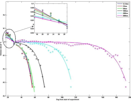
Fig. 4. Modeled variations of dilution rate with time based on the modeled total tracer volume.

(22)

OSD

6, 1735–1756, 2009

tracer

P. Xiu and F. Chai

Title Page

Tables Figures

◭ ◮

Back Close

Full Screen / Esc

Fig. 5.Linear relationship between b₂, derived from the exponential function fit, and the initial