A business cycle study for the U.S. from 1889 to 1982

(1)

t"

.

119 12

A 8US:ntBal

cYc%.B

.'IOD!" .

FOR

tu u.

S.

'"1"ROM

1889 TO

1912

by

(2)

-FOR mE U. S. l"ROM 1889 '1'0 1;82

by

Carlos Ivan Simonsen Leal*

*Prineeton Univerhity. helpful diseussions.

AprU 1984

I am very grateful to John Taylor for

(3)

I. The Model

Our aim is to aet up and eatimate a simllltllneous equations raHonal

expectations modelo We will work with three variables: product, wllge and

price 1evel.

As for the notation, capital letters will indicate nominal values,

amall letters e.te real value:!i. 1>.11 quant.ities, unless otherwise atated,

are expres!;tôé 1n logarithrne, Y at8nds for product, P fer price level, \-V

for wagt!', M for lIlt.1n!'y .Jnd t for time (not in log8). The use of a D means we are t8king the first difference, for example DP_t • P_t+_{1 - P}_t • Et

lndlcates expectation conditional on the information aval1able at time t,

and, for the matter of convention, we assume that a11 variables with

8ubscripts lese than or E>qual to t are contained 1n t-he information set at t.

lnspired by Barro [ l ] we assume that toe supply of product obeys

(1)

where we--and not Barro!--made the assumption that

nt

is a second order

mOving average processo

i~ a standard Lucas supply function. The new

hypothesis, tha 1t b~ing serielly correlated, cen bp. justified by s8y1 n9

(4)

where

The G~mand side of the econorn

_x

ia given by

J.l_t is a white-noise processo

We are assuming instant market clearing.

Some comments ought to be made about equations (1) and (2).

First, we don't estimate the coefficients aO' aI'

6

0, Sl •

(2)

We don't want to explain the trend, but only the fluctuations around it.

Of course, we are assuming a very particul~r form of trend, a linear trend;

we don't deny that and this is a flaw in our modelo

Second, ~e ~hould see equation (2) as fruit of an idea similar to

that of Keynes' c0nsumption function. In this case we should use ntW t instead of Wt , wh~r~ nt is a measure of the employed people. We don't

do so and since one has positive indication that nt ie growing with t ,

we expect

S2

to be a biased measute of the nominal wage effect.

Third, we said that nt i9 a second-order moving average process

while ia a white noise. _{The ideas here are two: we allow demand to}

adjust faster than supply and we use these constralnts to help identify

the model.

Fourth, one rnay find strange that we do not include a cash balance

effect In (2). We don 't do 90 because we want to study the power of

predlction and the good fitness of the medel if ignoring this type of

effect.

We assume that the economy follows the fOllowing wage

(5)

-

-4.

where agaln we ~on't hope to estimate neither

6

0 nor

6

1 , We see (5)

as a Inark-up equation í;;ubject to the random errors $ t ' As for Ô 2

we don't have any predjction cf signo Indeed, ô

2 can be seen as a prize for productivity, but a1so as the maximum discount effect that unexpected output wou1d have on wages. In the lfttter case of course we would be

admitting that_ unions are on1y but strong enough to lmpose a maxirnum rate

of di6count.

Our tasK now la to ta~e the equatíons we have, put the necessary

constr.lnts that haven't been put, and solve our rational expectations

modelo

vle s11a11 fir st intrüduce the following notation: a lO

k

c ..

k And, second, for the sale of clarity

w~ repeat her"! what we have, renurnbering the equations with letters:

(A)

nt

•

_°t+ 9

l0t-1 .... 92Ot_2 (Bl

y ,.

t

e

O + f31t .... S7Wt: + ₈3P" + u t (C)

W "" _t 6₀+ ₆₁t ₊_ô

2 (Yt - Et-1Yt' + p t + 4> t (D)

(6)

->

where

Using r~tional expectations we have for k > 2 that

b_k_{• b}₂ _{• h}_O+ h,t

J.

ho

B₂t5₀ + 8_{0 -} _ao

•

₈

2 + 83

h 1

•

(a_{l - aI)}~- 8₂6₁

f3₂ + 8

2

For k

=

1 we have

h •

. 3

(7)

6.

It ia our obligation to notice that what we are obtaining ls that

the on1y mechanism of a1tering expectations of future lnf1ations ia by the

transmlssion of errors and/or a1tering the coefficients h_{1, h2, h3 •}

111. Estimating the Model

where

Using the 1ag notation we can write the resultlng system as

2 A(L) • AO' B(L) • BO + B1L + _{B2L ,}

Zt •

_{(Yt' Pt , W}t ), e~ • (Ot' ~t' ~t) and

The matrices AO' BO' B₁, B₂ are given by:

A • _O

B : O

B -₁

I

i

L

1 1

-6

₂

.1 O

a

O 1 1 O 1

o

-e

₂

(8)

~. j9

2-a2h3 o

o

1

B

2

..

o

I

i "

~ .~'

o

_o

J

;:'3

'

-Now, insteaâ of estimating the vector ARIMA we will estimate

T

A(L'f r.. _{\"'t -} '" _{&<t-l -} ~

t-i-I

Zt_l

T ) .. BeL) (I-L)e

t

which ia a vector ARIMA for which I will use the Varma programo Notice

that We are using _{as a}

proxy for C_{1 ' what is clearly}

justified by the strong law of large numbers.Observe that S'm - Z,

.1. ;_.

..

----._.

T

The implication of the last paragraph 1s that we will only have estimates

for

_a

2 , ~2' ~3' 91 , 92, and

6

₂ ,

We point out that for the second period we had problema with having

Fisher's informe~ion rnatrix

RreO

)s1ngulnr and we had to proceed as

deE:;cribed in the appendix 1. There we showed the need to use the estimators

der ived from th{: prc:'~lei:

ma.'!: L(x,8j

(CE)

where L 15 the log-likelihood and TI

(9)

The results fite:

Coefficients

Cl2

S2

B.,

..

9 1 9 2

6

₂ Coefficients Cl₂

8

₂

6

₃ 9 1 9 2 Ô₂

FIRST PERIOO

(1889-1914 )

Es ti ma tes

0.467 -1.32 -2.€7 0.52 -0.15 2.33

SEcor.;o PERIOO •

(1909-1940) Estimates O 5.905 O 1.016 0.536 O 8.

Asymptotic T

2.98 -10 -8 2.68 -0.98 5.05

Asymptotic T

2.02

5.97

3.86

*We used thc constraint Cl2

=

6) •

Ô_{2 • O as a proxy for nkG. O.} This Was done by _{taking R (90) in the free estimation and Comput!ng its eigenvaL}

We found that the eigcnvalues corresponding to

a

(10)

THIRO PERIOO

(1953-1982)

Coefficients Estimates Asymptotic T

Q2 4.42 2.70

6

₂ 3.12 2.41

6)

-3.99 -3.23

8

1 0.83 6.16

9 ... 0.07 0.97

~

ó₂ -2.44 -8.00

We notice that for a11 periods Q2 is greater than or equal to zero,

in the first and last period supply falIe with expected inflation. Cl

2 =: O

in the second period was imposed in the estimation as a means of ru11ng

out the non-consisten~y of °the estlrnators obtained in the unconstrained

estimation.

6

2 has the sign opposite to what we expected in the fitst period, one very important point to be made is that in that period the U.S. was

receiving a huge masa of skilled 1abour at practically zero cost from Europe.

Then, if we could show that this exogenous growth of nt was negatively

correlated with W

t ' one would conclude that ff instead of using Wt

dy t ô.nt

in (2) we should have really used ntWt, then ~t·

6

₂ (n

t + WtêWt) and this number roay be negative. Of course, we are not glving a proof,

on1y a hint: it i8 usual to suppose that w

t ' the real wage, and nt

are negatively correlated if labour supply ia perfect1y elastic; but we are

supposing that W

(11)

,;,. ,.

10.

This will depend of course on how prices behave and we cannot obtain sny

suitable medel with the assumptions we hsve msde.

We csn reject

e,

+ 6

3 •

o ,

so that people see a raise in nominal as

actual increase ir. income.

We didn;t finJ any good explanation of the behaviour of

6

₂ , However,

we insist that one should look at the productlvity aneS discount effect

mentioned before.

Empirically the mede} WlJS very bad for the third period as tht'"

correlaticn table between actusl snd predicted values below shows.

PERIOD

VARIABLE 1st 2nd 3rd

Y

t 0.5462 0.4718 0.633

W_t 0.3221 0.1979 -0.55

P

t 0.2714 0.2628 0.0

Álso, for the third period we got the unpleasant festufe of gp-tting

e

t autocorrelated.

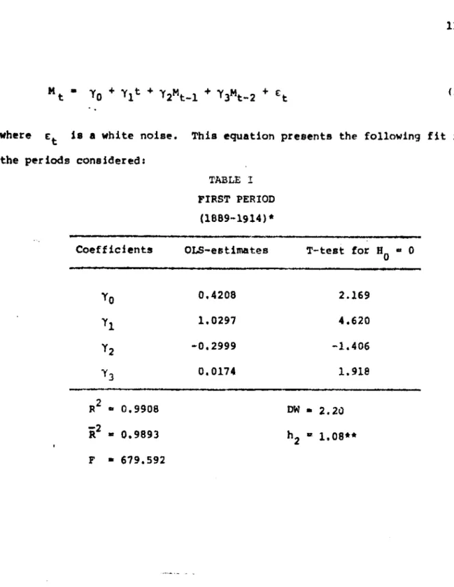
IV. A Note on the Money Marke~

-up to now we have not dealt with the money market and this may be one

of the reasons why we had such bad resulta for the third period.

Suppose that the equilibrium of the monetary market ia given by

(12)

---where

M • t

ia a

white noise.

the periods considered:

Coefficients

ro

11

1 2

)'3

R2 sr 0.9908

-2

R • 0.9893

F • 679.592

( 3)

This equation presents the following fit for

TABLE r

FIRST PERIOD

(1689-1914)

*

OLS-estimates

0.4208

1.0297

-0.2999

0.0174

T-test for BO a O

2.169

4.620

-1.406

1.918

DW • 2.20

*Because we don t t have enough observations we over1ap the 1st and 2nd pel

iadé-··h

(13)

Coefficients "1'0 I I

l2

l3

R 2 _

0.9806

-2

R _{- 0.9783}

F _{- 437.34}

Coefficients

"1'0

'Y₁

l2

"1'3

R2 • 0.9988

-2

R • 0.9986

F • 4959.38

TABLE 11

SECOND PERIOO

(1909-1940)

OLS-estimates

0.381

0.0043

1. 393

-0.512

TABLE 111

THIRO PERIOD

(1959-1982)"* OLS-estimates 0.745 0.010 0.826 0.023 12.

T-test for HO _{• O}

2.095

1.471

8.097

-3.000

ow-

1.914

h 2 • 0.934

T-test for HO - O

..

1.868

2.172

3.397

0.112

DW • 1.973

*Because we dontt have enough observations we overlap the 1st and 2nd periods.

·*h₂ is the correspondent of Durbin's h test when one has two 1ag8.

(14)

For alI three periods the fit is' very good and we point out that 2

À -

r

₂À -

r

_{3 • O always has dlfferent roots} À_1,À

2 , both lying inslde the unit circle. In this case, it 18 easy to verify that (3) can be

inverted into:

lJ t •

+

(4)

One immediate consequence of accepting (4) ia that the unexpected

component, of lJ t ia a white-noise. Another is that if we wrongly omit lJ t from (2) then the correlation imposed by the first two terms of (4) will transfer to lJ t ' giving the wrong impression that the lJt'C are correlated. The latter suggests that we rnight change our medel by changing

the hypothesis that lJ

t is a white noise. We ahal1 assume that lJ_t ia

a first order moving average process:

In this case, the medel we obtain coincides with the old one, except

(15)

14,

9₁

-a

₂h₂ Q2P O

13

₂

+13

₃-a₂

"

Sl • O P O

- 2h 2

₁₃

Q O

2

+13

3-Q2

It ia a wel1 known fact that increasing the order of an ARMA process

increaaes the good fitness of the mode1, but that this procedure la

mis1eadlng is a1so wel1 known. Looking at the correlation between actual

and predicted (one step ahead) va1ues we obtain the fo1lowlng tab1e:

PERIOD

VARIABLE 1st 2nd 3rd

Y_t _0.48086 _0.7414 _0.31463

W

t 0.40696 0.33564 0.84990

P

t 0.36024 0.58825 0.66818

Theonly sensible change 1s then on the third period. For th1s

(16)

Coefficients

Q2

8

₂

8

₃

9 1

9 2

6₂

P

V. Finê1 Remarks

THIRO PERIOO

(1953-1982)

Estimates

2.12

0.61

-0.92

0.74

0.12

-4.65

-0.31

Asymptotic T

2.08

3.73

4.12

1.99

0.70

-13.00

-3.39

By using theorem S in the appendix, one can establish a test for comparing

the coefficients across periods. We did this and the conclusion is that

there is no qualitative difference between the first and second periods. 50

that a

2

=

O, etc., sh~uld not be seen very seriously. We point out that this test has 10~' power because of the nurnber of variables minu9 the numbel' of

constraints with respect to the numher of observations. Also, because we d:::n ':

know the right order of moving average process involved, we are doomed to have

a biased testo

(17)

16.

Finally, the model assumes a very neutral govemment, one who has

an

almost b1ind monetary pOlicy. This is far trom reasonable and we think that

it explains the low power of prediction presented, thia ia obviously true

for the third period. Also, for the last period, there ls something more going

on, which is not captured by the model: there ia a change of the corre1ation

(18)

APPENDIX ' : ESTlMA'l'ION

.

One of the moat uaed theorems in Econometr iea ia the OM vhieh

aays that maximum likelihood estimatora (m.l.e.) uneSer certain condltiona

do converge in probab1l1ty to the true parameter of the dlatrlbution.

Our a1m 1n this appendlx la: f1rat, to atate the above theorem and

prove it in lts moat general fora, aecond, we vant to know what happena

when some of the eonditions ve uaed 1n the theorem are not true,

we

vill

be most lntereated 1n vhat happens vhen the information matrlx defined

below ls singular.

We atart by a lemma that vill prove uaeful:

!-e

mma 1: Glven an mxm positive sem1-definite matrix A we ean alwaya fineS

a positive definHe matrix A + such that for every v E (lerA).t "have

+

Av • A v •

Proof: _{the projectlon into the kernel of}_{A and define A • A(I-n}+

k,

+

n. Then, i'f v E (RerA).t , by defin1tion, _{nkv • O}_->_A+ _{v • Av.}_{On the other bend,}

1f v ~ O .. A+

o la positive definite.

With thls theorem ve can atate the famous °Carmer-Rao inequality 1n ita

most generalized formo But first we need to define the log-likel1hood

functipn.

Def1nition: Let xl"",xn be n lndependent identically distributed °random variables having density function f(x,9),

e

being a finite

dimensional vector of parameters, ve define thG· log-likelihood

n

function as L(xl'" t ,Xn' 9) ~ 1:, 109 f (Xi'9) •. o And for economy of notation

i-1 we aha11 write L(x,9) instead of L(x

(19)

18.

,.

A m.l.e. e i s , by definition, a value for e such that L(x,6).

is a maximum.

Theorem 1: (Cr:.:,)·:-:i.. ~ \<.a~f inequalltYJ

Suppose T i5 an unhiased estimator of e t that L(',9) ia lntegrable

and that: L(x,e) ie twice differentiable in 9 for almost a11 x. Then,

a

2

109 f ( 9)

if

R(e)

~

E (-

Xi'

ae'ae

)

is defined, we have

i8 positive semi-defini te.

The proof of this theorem can be obtained wit.h very l i ttle rnodificat.ic.lí.

r ....

from the one in Chow L 3

J

page 23.

Notice that what (A-li ia act.ually doing is setting a lower bound

for Cov T. We shall say that T i8 asymptotically efficient when

A characteriz~tion of A+ given A would be rnost desired here, We

however shall only indicate to the reader that the 'Way to characterize A +

passes througb using Jordan I s canonical form (see Hoffman-I<unze chapter 7

This i:1deed gives another proof of lemma 1. We shall see, however, that f~)t

our applications we 'Won't need lt.

There are two classical theorems of Probability theory that wc

(20)

theorem f: (Strong Law of Large Numbers)

Let

x

n ,be a sequt""C~ of independent and identically distributcd (i.i.d.) random variables. Then we have

W) 1im

n

r

X.;. .... EX 1

1"1 J. 1

n

Theorem 3: (Central Limit Theorem)

Let X

n be a sequence of Li.d. random variables w1th finite

non-singular covariance matrix COVX₁, then

ti

i!l (X_n-EX_l )

(- D

-t N (O,!)

where 1 ü> of the f.;2ll'l1e dimension of COVX₁ •

We are t1":n: '5':;lng to prove these two theorems. Their proof is

difficuH Clnd we suggf>st the rea~er the very good book of Chung [3

J .

Notlce that ln case COVX

1 Is not a scalar the notation

(CoVX1)-~

really means the matrix .H such that H'H· (CoVX1,-1 •

We now.pass to the usual resulte about convergence of m.l.e.'s.

Lemma 2: Suppose Ellog f (xi'9)

I

< Cc for a11 9 E.

n , n

compact conve",

that E 109 f(X_i ,9) h e~rictly concav~, cont1nuOU5 in 9

,

and that the samples. _{x 1 ,x2 ""} are i. Ld. Then we have:

a)

b)

for n big enouqh the set of m.l.e.'s in r is a singleton 9 f

(21)

• 20 •

!!22!:

For n blg enough the atrong 1aw of large numbera imp1les that

i·

1 1

- L(x 9) .

-n

'

n

18 atrictly concave a.e. for n big enough, thi.

impUea that ve on1y have one lI.l.e., 9

n • Slnee the 8n E

n

1ie on a compact set one can alwaya take a convergent aubaequence. Sinoe the .

..

xtmu.

of B 109 f(x,9) ia unique, any convergent aubaequence baa the

aue l1JDit 8₀ , Thia illlpHe a 8

n + 90 •

'l'heorell 4& Under the conditiona of lema 2 1f we auppoae 8

0 E int

n ,

that L ia twice differentiable and that R(9à) ia defined and positive

definite, we have that the 9_{n are aaymptotically efficient and} a.~totically

.. normal.

Proof:

-vhere

'l'he m.l.e. 8

n ia a aolution to a9 (x,e

l!!

_n, • O , use this to wfite

a(9

n - 80)

119

n - 80

11

• O •

'l'hen multiply thia equatlon by R(8J-l

and take the limit when n + ~ •

_By

_{the atrong lav}

n

1 _R(e -1

a

2L

O'

<aetas (x,eO

» a.8. -1 and by the Central Limit theorem, aince

COv(~)

• R(9

0"

we

hav. that

Nothingup to now indicatea that e

O ia the true parameter of the

d~stribution. Indeed, whet ia uaually done ia to tate thia hypothesia and

give no further juatification. Wh~t happcns then when ve don't have

convergence assured? 'l'he obviou. ans~~er has to come froll the analyals of

lemma 2 above. Ne vill only look at t:he condition .aying that E 109 feXi,e)

ia atrictly concave in e .

FUNDAÇÃO GETOUO VARGAS

8iblioteca M2ri~ }"{.:·'''ri~' .. ie Simonsen

(22)

Now, i f Wt! want to avoid technical problems that ~·.'ill only difficl,1lt

the proofs, b~t not change the spirit of the results, we will allow L to

be twice differentiable. Suppose, then, that we solve

rr'1X L (x.e)

s.L Ii

k9 .. O

where here TI

k i5 the projection on the kernel of RClb)' It ia easy to ck,,·

that L i8 atr ict1y concave outside the kernel of R (9

0) and so we can

mimic lemma 2 to find estimators 9

n with limit 90 , the only

difference being that now TI

k90 • O. Theorem 4 can be copied too, however,

we need to take some care: first the fhst order condition for maximizatior

ia now given by

where

because

~

_ae

(x

_'

e )

=

n' ,

n k /\

À

=

U1,···,À_m) 1s a vector

of this (A-2) ie written

of lagrange multipliersJ

TI')., 2L (X/AO) d

2 L

(x,eo' (en - eo) +

o(e

n - 90>

~

...

- +

-k (lP de' ae

. Multiplying this eqllality by (e

n - 90)' (R{eo)+,-l we have

Sut this implies

(A-3)

(23)

+- -1 + 1 ,,2t

( R(a

O) ,', .. ú-0-:' R • IX, e ) O' + (R(r..»-U

o

o dO'dO ( O )(9 e ) x,

o

m-

o

-> (1 -

n)

(R(8 )+,-1 aL (x/po) +

k

o

ae

+ (I - TI ) _k 0(9 -9 ) • _n

_o

o

and, then, using the strong law, the Central L1mit Theorem and the fact

that (R(eo,+)-l R(G

O) - I -

n

k we conclude that:

(A-4)

22.

The D-Jimit above 18 the maximum one can say when R(9

0, 15 singular

using this kind of technique. Suppose we want to test "O : atrue

=

_{9 0} against R

1 : atrue ~ 91 T using (A-4) above what we actua11y obtain i8 a cylinder corresponding to the perpendicular translation of the confidence

region in ker R(9

0, obtained by testing the positive components of

(I - TI

k) (en - 91) • This indicates that the power of (A-4) should not

be very good.

The problem ia then to find another test for which we would have good

power. The answer was given by HaUS8man ([4

J),

or1ginally he studied the

following situation: suppose we have a medel

y •

XS

+

Xa

+

v

(A-5)

(24)

information is given about the v's, if the v's are correlated with

~

i],

etc, thi'J result was the following theorem:

"

""

Theorem 5: Suppose w(> have two estimators 90' 91 both consistent and

asymptotical1y normal1y distributed with 9

0 attaining the asymptotic

Cramer-Rao bound. Let, a180, m be the number of coordin~tes in

each of these cOo~dinates, q . (9

1 - pl~m 91) - (90 - plim 90, and

M· V(9₁) - V(8₀), where V indicates the covarianee matrix, then

where k · m - dirn (ker M)

To complete thia appendix we extend Durbin's h-test, see Chow

[2 ]

page 85 , to the case where one haa s lagged dependent variables on the

r ight hand side of a regression Y" XB + lJ and wanta to test if j.I i5

autocorrelated. The basie reference is Breush ar.d Pagan [5 ] . There the

authors by uS11'1g Lagrange estimators conclude that i f ooe lias the model

y • X8 + ~, X la NxK

j.I ..

t P' I I-'t-l + et

where e_t '\. N(O,o I), 2 one has that the null hypothesis HO p _{• O , ean}

be tested by using the statistic

where: j.I " I • (lJN,···,lJ,.. ,.... _{s +}_{2}' lJ_ 1 • (UN- 1},.., ""

,···,lJ

,.. _{s +}_{1 )} the " indicating

that is estimated under

"o·

O (OLS) 1 and r2 ''', -1'"

"'-1

=

(j.I~) ~~l~'

They prove that T

~

Xi .

Our task then ia just to calculate the plim of

the s 18g8 condition. We partition X into two mat.ri~e5 X a (X,X ),

e ne

(25)

,

-YN- l YN-2 'l _N-a

X

..

_'lN-2 _YN-3

. ..

'l

e N-s-l

'/8+1

...

'l1

...

-t

'l

-1 y -2 t • • • • • • • • • •

Now given that

~I-l·

lo\' -1 ' where M· I - X (X'X) -lX' , we use the

Weak Law of Large Numbers to get

'l'

_t+.i

-1 p

-.1

..

₁

"-2

O N

'l' _{M:i_}

2 P -1

1'3

1

"

..

"'-2 N

O

'l' _My-s

li -1

6.-

1

'"

-2

..

O

'l' M X

~

and _{Ã_?}-1. -21.!:- O

O - N

where 1'3

1'."

,f:\;

are the coeffjcients af Yt -1, Yt- 2 ,···, Yt -s '

For the case S " 2 we have

2 Nr

l T" ---

.----~---~--'" A A '" A2 A

G

+ Cov

13

1 +

2af

Cov(J3. 1

,a

2 ) +

6

1 Cov8 2 ]

(in the text h

(26)

[5

J

BIBLTOGRAPHY

..

R. Barro, Introduct.ion .to ManeJo, Ex,r:ectat.ions 8pd BusJne~s Ci:ç.!f..~, Acadernic Press, 1981.

IC. Chung, ~_SSm.E.!H! ,in. 'p!obabilit:t, tl}"f!9~, Academic Press, 1968.

J. Haussman, Specificatlon Teste in Econometrics, ~conometrlc~, volt 46, 1978, pages 1251-1275.

T. S. Brensh and A. R. Pagan, The Lagrangc Multiplier Test and Its Appl1cations, ~, XLVII, 1980, pages 239-2S3.

(27)

ENSAIOS ECONOMICOS DA EPGE

1. ANALISE COMPARAT/iA DAS ALTERNATIVAS DE POlrTICA COMERCIAL DE UM PAIS EM

PRO-CESSO DE

INDUSTRIALIZAÇ~O

- Edmar Bacha - 1970 (ESGOTADO)

2. ANALISE

ECONOM~TRICA

DO MERCADO INTERNACIONAL DO

CAF~

E DA POLTTICA

BRASILEI-RA DE PREÇOS - Edmar Bacha - 1970 (ESGOTADO)

3. A ESTRUTURA ECONOMICA BRASILEIRA - Mario HenrIque

Sln~nsen

- 1971 (ESGOTADO)

4. O PAPEL DO INVESTIMENTO EM

EDUCAÇ~O

E TECNOLOGIA NO PROCESSO DE DESENVOLVIMEN

TO ECONOMICO - Carlos Geraldo Langonl - 1972 (ESGOTADO)

-5.

A EVOLUÇXO DO ENSINO DE ECONOMIA NO BRASIL - Luiz de FreItas Bueno - 1972

6. POLTTICA ANTI-INFLACIONARIA - A CONTRIBUIÇAo BRASILEIRA - Mario Henrique

SI-monsen -

1973

(ESGOTADO)

7. ANALISE DE

S~RIES

DE TEMPO E MODELO DE

FORMAÇ~O

DE EXPECTATIVAS - José

Luiz

Carvalho -

1973

(ESGOTADO)

8. DISTRIBUIÇXO DA RENDA E DESENVOLVIMENTO ECONOMICO DO BRASil: UMA

REAFIRMAÇ~O

Carlos Geraldo Langonl - 1973 (ESGOTADO)

9. UMA NOTA SOBRE A

POPULAÇ~O

OTIMA DO BRASIL -

Edy

Luiz Kogut - 1973

lO. ASPECTOS DO PROBLEMA DA

ABSORÇ~O

DE MAO-DE-OBRA: SUGESrOES PARA PESQUISAS

José Luiz Carvalho - 1974 (ESGOTADO)

lI. A FORÇA 00 TRABALHO NO BRASIL - Mario Henrique Slmonsen - 1974 (ESGOTADO)

12. O SISTEMA BRASILEIRO DE INCENTIVOS FISCAIS - Mario Henrique Slmonsen - 1974

(ESGOTADO)

13. MOEDA - AntonIo Marta da SIlveira - 1974 (ESGOTADO)

14. CRESCIMENTO 00 PRODUTO REAL BRASILEIRO - 1900/1974 - Claudio Luiz Haddad

(28)

16. AN~LISE

DE CUSTOS E BENEFTclOS SOCIAIS I - Edy Luiz Kogut - 1974 (ESGOTADO)

17. DISTRIBUICÃO

DE REND/\:

RESUMO

'DA

EVIDENCIA - Carlos Geraldo Langonl - 1974

(ESGOTA.DO)

18.

O

MODELO ECONOMtTRICO

f'F

5T,

LOlJIS

APLICADO NO BRASIL: RESULTADOS PRELlMINA

RES - A.ntonio Carlos Lemgruber -

J9jS

19. OS MODELOS

CL~SSICOS

E

NEOCLAsSICOS DE DALE W, JORGENSON -

EI (seu

R.

de

An-drade Alves - 1975

20. DIVID:

11M. PROGRA'-~

FLEXrVEL PARA

CONSTRUÇ~O

DO QUADRO DE

EVOLUÇ~O

DO ESTUDO

DE UMA DrVIDA - Clovis

de

Faro - 1974

21.

ESCOLHA, ENTRE OS REGIMES DA TABELA PRICE E DO

SISlEW, C/[

AMORTIZAÇOES CONSTAN

TES: PONTO-DE-VISTA DO MUTUARIO - Clovis

de

Faro -

1975

-22.

ESCOLAR,IDADE, EXPERIENClt\ NO TRABALHO E SALARIOS NO 8RASIL • José Julio

Sen'"

na -

1975

230

PESQUISA QUANTITATIVA NA ECONOMIA - Luiz de Freitas 8ueno - 1978

24. UMA ANALISE EM CROSS-SECTION DOS GASTOS FAMILIARES EM CONEXAo COM

NUTRIÇAO~

SAODE, FECUNDIDADE E CAPACIDADE DE GERAR RENDA - José Luiz Carvalho - 1978

25'.

DETERMINAÇAo DA TAXA DE JUROS I MPLfc /TA EM ESQUEMAS

GEN~R

I COS DE FI NANe

lA-MENTO:

COMPARAÇ~O

ENTRE OS ALGORTTIMOS DE WILD E DE

NEVTON-~PHSON

- Clovis

de Faro - 1978

26. A

URBA~IZAÇAo

E O CrRCULO VICIOSO DA POBREZA: O CASO

~

CRIANÇA URBANA NO

BRASIL - José Luiz Carvalho e Urlel de Magalhães - 1979

27. MICROECONOMIA - Parte I - FUNDAMENTOS DA TEORIA DOS F'REÇOS • Mario Henrique

Slmonsen - 1979

(29)

29.

CONTRADIÇ~O

APARENTE - Octávio Gouvêa de Bulhões - 1979

30.

MICROECONOMIA - Parte

2 -

FUNDAMENTOS

DA

TEORIA DOS PREÇOS - Mario Henrique

Slmonsen -

1980

(ESGOTADO)

31. A

CORREÇ~O MONET~RIA

NA JURISPRUDtNCIA SRASILE:IRA - Arnold Wald - 1980

32. MICROECONOMIA - Parte A - TEORIA DA DETERMINAÇAO DA RENDA E DO NfvEL DE PRE

ÇOS - José Julio Senna - 2 Volumes - 19BO

33. ANALISE DE CUSTOS

E

BENEFTclOS SOCIAIS II I - Edy Luiz Kogut - 1980

34. MEDIDAS DE

CONCENTRAÇ~O

- Fernando de Holanda Barbosa - 1981

35.

CR~DITO

RURAL: PROBLEMAS ECONOMICOS E SUGESTOES DE MUDANÇAS - Antonio

Sala-zar Pessoa Brandão e Urlel

de

Magalhães - 1982

36.

DETERMINAÇ~O NUM~RICA

DA TAXA INTERNA DE RETORNO: CONFRONTO ENTRE ALGORfTI

MOS DE BOULDING E

DE

WILD - Clovis de Faro - 1983

37. MODELO DE EQUAÇOES SIMULTANEAS - Fernando de Holanda Barbosa - 19B3

38. A EFICIENCIA MARGINAL DO CAPITAL COMO CRIT(RIO DE

AVAlIAÇ~O ECONO~ICA

DE PRO

.

JETOS DE INVESTIMENTO - Clovis de Faro· 1983 (ESGOTADO)

39. SALARIO REAL E

INFLAÇ~O

(TEORIA

E

ILUSTkAçAO

I~MPrRICA)

- Raul José Ekerman

- 1984

40. TAXAS DE JUROS EFETlVAMENTE PAGAS POR TOMADORES DE

EMPR~STIMOS

JUNTO A

B~

tOS COMERCIAIS - Clovis de Faro - 1984

41.

REGULAMENTAÇ~O

E DECISOES DE CAPITAL EM BANCOS COMEkCIAIS:

REVIS~

DA L1TE

RATURA E UM ENFOQUE PARA O BRASil - Urlel de Magalhães - 1984

-42.

INDEXAÇ~O

E AMBltNCIA GERAL DE NEGOCIOS - Antonio Maria da Silveira - 1984

(30)

"4.

SOBRE O NOVO PLANO DO BNH: IISIHC"*- ClovIs de Faro -

1984

45. SUBsTDIOS CREDITTclOS

~

EXPORTAÇXO - Gregório F.lo Stukart - 1984

460 PROCESSO DE DESINFLAÇXO - Antonio C. Porto Gonçalves - 1984

47. INDEXAÇXO E

REALIHENTAÇ~O

INFLACIONARIA - Fernando de Holanda Barbosa - 19Bq

48. SAlARIOS

M~DIOS

E SALARIOS INDIVIDUAIS NO SETOR INDUSTRIAL: UH ESTUDO DE DI

FERENCIAÇAo SALARIAL ENTRE FIRMAS E ENTRE

INDIVrl~OS

- Raul José Ekerman

e

UrJel de Magalhães -

1984

49. THE DEVELOPING-COUNTRY DEBT PROBlEM - Mario Henrique Slmonsen -

1984

50. JOGOS DE INFORHAçAO INCOMPLETA: UMA INTRODUÇXO - Sérgio RibeIro da Costa

Werlang -

1984

51. A TEORIA MONETARIA MODERNA E O EQUILTBRIO GERAL WALRASIANO COM UH NOMERO

INF1NITO DE BENS -

Ao

Araujo -

1984

52. A INDETERMINAÇAo DE MORGENSTERN - Antonio Maria da Silveira -

198q

53. O PROBLEMA DE CREDIBILIDADE EM POLTTICA ECONOMICA Rubens Penha Cysne

-.1984

54. UMA ANALISE ESTATTsTICA DAS CAUSAS DA EMISsAo DO CHEQUE SEM FUNDOS:

FORMU-lAÇA0 DE UM PROJETO PILOTO - Fernando de Holanda Barbosa, Clovis de Faro e

Alofslo Pessoa de Araujo -

1984

55. POLTTICA MACROECONDMICA NO BRASil: 1964-66 -

Rubens Penha Cysne - 1985

56.

EVOLUÇ~O

DOS PLANOS BAs I COS DE F I NANC I AMENTO PARA AQU I SI çAo DE CAS.A PROPRI A

DO BANCO NAC IONAl DE HAB I

TAÇ~O:

1964 -

1984. -

C1 avi s de Fêlro -

1985

57. MOEDA INDEXADA - Rubens P. Cysne - 1985

(31)

59. O ENFOQUE MONETARIO DO BALANÇO DEPAGAHENTOS:

UH RETROSPECTO - Valdir Rlimalho

'

de Melo - 1985

60. MOEDA E PREÇOS RELATIVOS: EVIDENCIA EMPTRICA - Antonio 5alazar P. Brandão ,_

1985

61.

INTERPRETAÇ~O

ECONOMICA.

INFLAÇ~O

E

INDEXAÇ~O

Antonio MarIa 'da Silveira

-1985

62, MACROECONOMIA - CAPITULO I - OSISTEHA HONETARIO - Harlo Henrique Slmonsen

e Rubens Penha Cysne -

1985 '

63. MACROECONOHIA - CAPTTULO

ti -

O BALANÇO DE PAGAMENTOS

-Slmonsen e Rubens Penha Cysne -

1985

Karlo Henrique

6~.

HACROECONOMIA - CAPTTULO III - AS CONTAS NACIONAIS -

Harfo Henrique Slmonsen

e Rubens Penha Cysne - 1985

65. A DEMANDA POR DIVIDENDOS: UMA JUSTIFICATIVA TEORICA -

T~

Chln-Chlu Tan e

Sergio Ribeiro da Costa Werlang -

1985

66. BREVE

RETROSPE~TO

DA ECONOHIA BRASILEIRA ENTRE

1919

e

J98~

• Rubens Penha

Cysne -

1985

61. CONTRATOS SALARIAIS JUSTAPOSTOS E POLrTICA ANTI-INFLACIONARIA'· Mario Henrique

Slmonsen -

1985

68. INFlAçAO E POLfTleAS DE RENDAS - Fernando de H01anda Barbosa e Clovl. de

Faro -

1985--69 BRAZIL INTBRNATIONAL 'l'RADB AND 'ECONOMIC

GXMm -

Mario

Henrique

Si~n8en

-

1986

70. CAPITALIZAçAO CONTfNUA: APLICAÇOES - Clovis de Paro -

1986

71.

A

RATIONAL EXPECTATIONS PARADOX -Mario Henrique

SJaonaen -

1986

72. X BUSlNESS CYCLE STUDY roR THE U.S. FOJM 1889 TO 1982 - Carlos IvanSillOnaan

Leal - 1986

000046471