www.ocean-sci.net/8/319/2012/ doi:10.5194/os-8-319-2012
© Author(s) 2012. CC Attribution 3.0 License.
Ocean Science
137
Cs off Fukushima Dai-ichi, Japan – model based estimates of
dilution and fate
H. Dietze and I. Kriest
IFM-GEOMAR, Leibniz Institute of Marine Sciences, D¨usternbrooker Weg 20, 24105 Kiel, Germany
Correspondence to:H. Dietze ([email protected])
Received: 26 May 2011 – Published in Ocean Sci. Discuss.: 21 June 2011 Revised: 25 April 2012 – Accepted: 7 May 2012 – Published: 5 June 2012
Abstract. In the aftermath of an earthquake and tsunami
on 11 March 2011 radioactive137Cs was discharged from a damaged nuclear power plant to the sea off Fukushima Dai-ichi, Japan. Here we explore its dilution and fate with a state-of-the-art global ocean general circulation model, which is eddy-resolving in the region of interest. We find apparent consistency between our simulated circulation, estimates of 137Cs discharged ranging from 0.94 p Bq (Japanese Govern-ment, 2011) to 3.5±0.7 p Bq (Tsumune et al., 2012), and measurements by Japanese authorities and the power plant operator. In contrast, our simulations are apparently inconsis-tent with the high 27±15 p Bq discharge estimate of Bailly du Bois et al. (2012).
Expressed in terms of a diffusivity we diagnose, from our simulations, an initial dilution on the shelf of 60 to 100 m2s−1 . The cross-shelf diffusivity is at 500±300 m2s−1significantly higher and variable in time as indicated by its uncertainty. Expressed as an effective resi-dence time of surface water on the shelf, the latter estimate transfers to 43±16 days.
As regards the fate of137Cs, our simulations suggest that activities up to 4 mBq l−1 prevail in the Kuroshio-Oyashio Interfrontal Zone one year after the accident. This allows for low but detectable 0.1 to 0.3 m Bq l−1entering the North Pa-cific Intermediate Water before the137Cs signal is flushed away. The latter estimates concern the direct release to the sea only.
1 Introduction
0 2500 5000 10
50 100 150 200 250
Depth [m]
∆
z
[m
]
(b)
[km]
[m]
(a)
(d) (c)
Izu Ri d g e Honshu
Hokkaido
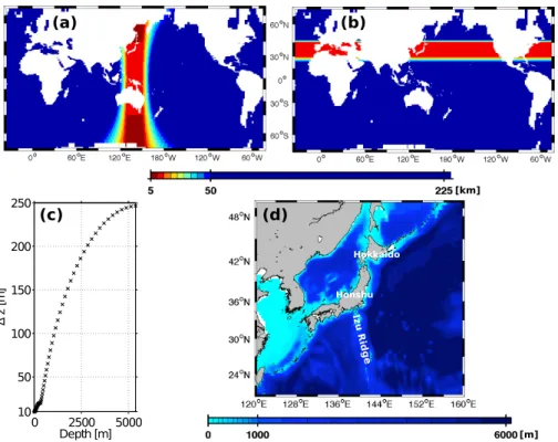
Fig. 1.Model grid. Panels(a)and(b)are horizontal and meridional resolution, respectively. Panel(c)shows the vertical resolution1zas a
function of depth. Panel(d)shows the model bathymetry in the region of interest (white areas are considered as land by the model while the grey patches outline the actual land distribution).
observations, and (2) to come up with a quantitative measure of dilution or effective residence time of137Cs on the shelf. Such a measure could be of interest to studies to come with a focus on, e.g. marine biota off Fukushima that do not want to afford the computational expenses of ocean circulation mod-els. Finally, (3) to explore the fate of137Cs released after one year.
In the following section we describe our main tool, the ocean general circulation model, and the numerical tracer re-lease experiments. In Sect. 3.1 time averaged quantities of the circulation model are compared with observations. Sec-tion 3.2 compares simulated surface currents and137Cs ac-tivities with actual conditions. Section 4 presents a model projection of how the137Cs is diluted onto basin-scale, fol-lowed by quantitative estimates of diffusion in Sect. 5. Re-sults are discussed and summarized in Sect. 6 and Sect. 7, respectively.
2 Method
2.1 Circulation model
We use the MOM4p0d (GFDL Modular Ocean Model v.4, Griffies et al., 2005) z-coordinate, free surface ocean gen-eral circulation model. The configuration covers the entire global ocean with an enhanced meridional and zonal reso-lution around Japan. Figure 1a and b show the zonally and
meridionally varying resolution. The vertical grid, with a to-tal of 59 levels is shown in Fig. 1c. The bottom topography, shown in Fig. 1d, is interpolated from the ETOPO5 dataset, a 5 min gridded elevation data set from the National Geo-physical Data Center (http://www.ngdc.noaa.gov/mgg/fliers/ 93mgg01.html). We use partial cells.
After a spinup of 5 yr, covering the period 1993 to 1998, the clock assigning the model forcing is reset to 1993 and the model is integrated for another 5 yr. In this second period the model tracers are released as described in the next section (Sect. 2.2). The period 1993 to 1998 is an arbitrary choice. Ideally, we would drive the circulation with actual, realistic fluxes. But even then, due to uncertainties in the initial con-ditions and the highly non-linear dynamics of ocean eddies, it would be impossible to make an exact hindcast without setting up complex data assimilation machinery. In order to account for this deficiency in our approach we explore an en-semble of tracer release experiments. The experiments differ with respect to initial conditions and the forcing.
In all other respects, not described here, the model config-uration is identical to the configconfig-uration without data assimi-lation described by Oke et al. (2005) and used, e.g. by Dietze et al. (2009). It is furthermore, except for the grid, identical to the configuration used in Liu et al. (2010).
2.2 Tracer release
In order to simulate the accidental release of137Cs, we em-bedded (online) an artificial tracer into the MOM4p0d circu-lation model. The tracer is released into a surface grid-box comprising 10×10 km next to the location of the nuclear power plant Fukushim Dai-ichi (Fig. 2). The tracer is conser-vative, i.e. it does not decay but behaves like a dye, subject to mixing and advection only. On timescales much shorter than the≈30 yr half-life of137Cs the behavior of our artifi-cial tracer mimics that of137Cs.
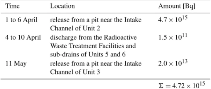
The total, direct release of137Cs from land to sea is uncer-tain. The Japanese Government lists 3 major releases totaling four to five peta Bq in a report to the International Atomic Energy Agency (IAEA) (Table 1). The associated fraction of discharged137Cs activity is reported as 0.94 peta Bq in at-tachment VI-1. Most of this estimated discharge is based on visual records of the flying distance of contaminated water flushing out of a duct.
In contrast, the “Institut de Radioprotection et de sˆuret´e nucl´eaire” (IRSN) states that “... 2.3×10¹⁵Bq of137Cs could have been released into the sea” (IRSN, 2011), but their un-derlying database and reasoning is unclear. Even higher esti-mates, 3.5±0.7 p Bq and 27±15 p Bq, are published in peer reviewed journals by Tsumune et al. (2012) and Bailly du Bois et al. (2012), respectively. They are based on an ad-justment of discharge such that simulations with an eddy re-solving circulation model compare well with observations (Tsumune et al., 2012), and on the temporal evolution of 137Cs content in seawater within a 50 km area around the damaged power plant (Bailly du Bois et al., 2012). While the amount differs by almost a factor of 30, all estimates agree that most of the discharge was confined to a period of the or-der of a week: i.e. within the period 1 to 6 April according to Japanese Government (2011) (Table 1), more than 60 % in the period 23 March to 6 April according to Tsumune
1 2 3
5 6
7
8 9
10 11 12
13
14 16
17
1819 20
[S!1] [S!2] [A]
[B] [1] [2] [3]
[4]
[5] [6]
[7]
[8] [9] [10]
[S!3] [S!4]
40’ 50’
141oE 10’ 20’ 30’ 37oN
12’ 24’ 36’ 48’
Fig. 2. Map of 137Cs observations and model grid. The black
crosses indicate measurements by TEPCO, the black x those by MEXT and the red x marks the nuclear power plant. The grey squares indicate “wet” model grid-boxes. In Fig. 7 and Fig. 8 the observations are binned into their nearest “wet” model grid-box neighbor. The TEPCO positions carry a reading error because they are copied from a map. The red dashed line in the lower right corner is the 200 m isobath.
et al. (2012), and more than 80 % in the period 26 March to 8 April.
In our simulations we release a total of 2.3×10¹⁵ Bq of 137Cs. We do not account for air–sea fluxes of137Cs. Choos-ing the IRSN (2011) estimate is a pragmatic decision trig-gered by the fact that it is the median and almost exactly the mean of all lower (compared to the Bailly du Bois et al., 2012) estimates. It is not a statement concerning the cred-itability of the IRSN (2011) estimate. Please note that a more comprehensive discussion on the amount of137Cs discharged to the sea and the effect of air–sea fluxes is given in Sect. 6.
As for the timing of the simulated discharge our choice is also pragmatic. As mentioned above all estimates agree in that most of the discharge was confined to a period of the order of a week sometime between 26 March and 8 April. All of our simulations feature an instant, meaning from one time step to another, discharge on 1 April. An additional ex-periment with all137Cs released instantly to the ocean one week later on 8 April 1993 yields, when compared to the 1 April 1993 discharge simulation, a measure of that uncer-tainty that is related to uncertainties concerning the exact time(s) of137Cs discharge.
Table 1.Estimate of radioactive materials discharged to the sea at Fukushima Dai-ichi nuclear power station according to Japanese Government (2011).
Time Location Amount [Bq]
1 to 6 April release from a pit near the Intake Channel of Unit 2
4.7×10¹⁵
4 to 10 April discharge from the Radioactive Waste Treatment Facilities and sub-drains of Units 5 and 6
1.5×10¹¹
11 May release from a pit near the Intake Channel of Unit 3
2.0×10¹³
6=4.72×10¹⁵
5 tracer releases, each one starting with all137Cs discharged into the ocean on 1 April of the nominal model years 1993 to 1997. This ensemble is compared with geostrophic velocities as derived from space observations during the actual time of the accident (Sect. 3.2). This evaluation reveals which of the nominal model years features a circulation similar to the actual conditions at the time of the accident.
3 Model evaluation
3.1 Time averaged surface currents, eddy kinetic
energy and surface mixed layer depth
The aim is to demonstrate that the circulation model shows reasonable realism as is to be expected from todays’ eddy-resolving general ocean circulation models. To that end a comparison with observed temperature and salinity does not provide much insight because (1) the thermocline does not deviate much from the initial, climatological, conditions in the short (5 to 10 yr) simulation period presented here, and (2) we restore both temperature and salinity at the surface (Sect. 2.1) thereby forcing a close match to observations.
More meaningful is a comparison with surface geostrophic currents as estimated from space. We use analyses based on pioneering work from Ducet and LeTraon (2001) and what have become known as the “Archiving, Validation, and Interpretation of Satellite Oceanographic data (Aviso, CNES)”. Aviso maps of absolute geostrophic velocities and geostrophic velocity anomalies are available on a 1/3×1/3◦ Mercator grid with weekly resolution. According to Ni-iler et al. (2003) these surface geostrophic currents show a good agreement (correlated at 0.8), with estimates based on drifters in the Kuroshio Extension region (25–42◦N, 142–
180◦E) in the 1990’s. In Fig. 3 the Aviso data are compared with modeled surface currents. The Ekman current is not sub-tracted from the modeled currents. This is a minor issue be-cause the Ekman currents are typically much smaller than the eddy currents, and the Kuroshio is essentially in geostrophic balance (Uchida et al., 1998). Hence, we conclude that most of the misfit between model, and observations offshore is due
to deficient model dynamics. However, this might not apply near the coast where the assumption of geostrophy might be rendered invalid by bottom friction and degraded accuracy of Aviso data.
That said, the agreement between model and observation is remarkable in the region of interest off Fukushima. Namely the main features described by Niiler et al. (2003) are in good agreement: the Kuroshio Extension jet is deflected north-wards after crossing the Izu Ridge (Fig. 1) and at a bot-tom trough at 35◦N, 150◦E. The Tsugaru current flowing eastwards between Honshu and Hokkaido, divides into two branches. One branch feeds a near-coastal current flowing southwards to about 36◦N. The other branch merges with the northeast oriented Oyashio frontal current.
The recirculation cells of the Kuroshio south of 36◦N are,
on the other hand, not well simulated by the model. But since (as will be shown later) the released137Cs does not cross the Kuroshio at the surface in our simulations, this misfit should be irrelevant.
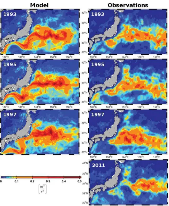
Figure 4 shows a comparison between simulated and ob-served (as derived from Aviso geostrophic velocity anoma-lies) eddy kinetic energy (EKE), which characterizes the mesoscale activity. It is defined by
EKE=0.5 u′2+v′2
, (1)
where u′ and v′ are deviations of the zonal and merid-ional surface velocities from their time mean (one year in this case), respectively. The overbar denotes a temporal av-erage over one year, u′ and v′ are weekly snapshots (for both model and observations). The simulated EKE is sim-ilar to the observed one in the region of interest (east of 140◦E) although, overall, biased high. Typically the
Fig. 3.Surface currents, averaged over the period 1994 to 1996. The color shading denotes absolute velocity. The arrows indicate the direction of the currents. The magenta line is the 200 m isobath. Panel(a)shows simulated velocities. The actual model resolution is three times higher (in both meridional and zonal direction) than indicated by the arrows. Panel(b)shows geostrophic velocities as estimated from space (Aviso, CNES).
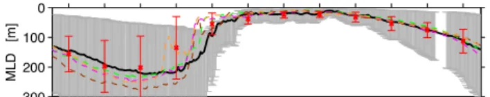
In addition to horizontal surface currents, vertical mixing affects137Cs activities at the surface. On the monthly to sea-sonal timescales considered in this study, vertical mixing is dominated by surface mixed layer dynamics. A direct com-parison of surface mixed layer depths is complicated by its extremely high variability both in space and time. This vari-ability is, predominantly, a result of the strong eddy activity (compare Fig. 4): the formation and intensification of anti-cyclonic eddies is accompanied by downwelling fed by the convergence of horizontal surface currents, which deepen the surface mixed layer. For cyclonic eddies, on the other hand, the reverse holds: formation and intensification comes along with a divergence of horizontal surface currents which pulls up the isopycnals and results in shallower surface mixed lay-ers. Figure 5 compares a regional average of modeled surface mixed layers with data obtained from profiling Argo floats; given the high variability in both model and observations, the model is consistent with the observations.
3.2 Surface currents at the time of the accident and
137Cs activities on the shelf
We aim to simulate the dilution and cross-shelf transport of 137Cs discharged off Fukushima Dai-ichi. This task is com-plicated by the temporal variability of surface currents on spatial scales including that of the size of the shelf (≈40 km). It is straightforward to assume that this variability is consid-erable for the task at hand, given that the meso-scale activity in the region ranks among the highest world-wide. Hence, the consistency between simulated and observed temporal or spacialaveragesdemonstrated in Sect. 3.1 does not necessi-tate a realistic simulation at a given time. Or, in other words, a simulated state of the eddying circulation similar to actual conditions is a precondition for successfully simulating the
accidental137Cs discharge in April 2011. This, fortunately, turned out not to be as hopeless as the combination of chaotic eddy dynamics and the fact that we do not assimilate real-time data suggests.
The reason why we are able to come up with a rather re-alistic simulated state of the circulation (despite vivid eddy dynamics) is that, apparently, only two contrasting states of the circulation prevail in the region. Both, visual inspection of sea surface height data (Aviso, CNES) and our simula-tions imply that there is a state where the average movement of surface water on the shelf is southbound. This state seems to be controlled by the southbound near-coastal branch of the Tsugaru current, and prevailed also at the time of the accident and in the nominal model years 1993 and 1996 (upper row of panels in Fig. 6).
The other state of circulation is showcased by observations on 12 March 1997 (lower left panel in Fig. 6) where the av-erage movement of surface water on the shelf is northbound, apparently effected by an anti-cyclonic eddy shed off by the Kuroshio current. Similar patterns, i.e. an average northward surface velocity on the shelf effected by an instability or a meander originating from the Kuroshio is simulated in the nominal model years 1994, 1995 and 1997.
We conclude that the simulations labeled with the nominal model years 1993 and 1996 are well suited to simulate the fate of137Cs discharged in April 2011 since they mimic the actual conditions, namely the average southbound movement of surface water on the shelf.
Fig. 4.Eddy kinetic energy as defined by Eq. (1). The left row of panels refers to simulated nominal years indicated in the respective upper left corners. The right row refers to estimates based on geostrophic velocity anomalies as observed from space. Due to lagged data access, the 2011 observations refer to an average from September 2010 to September 2011.
taken by TEPCO (Tokyo Electric Power Company) and dig-itized from an International Atomic Energy Agency presen-tation titled “Marine Environment Monitoring of Fukushima Nuclear Accident (2 June 2011) – Presentation Transcript” by H. Nies, M. Betti, I. Osvath and E. Bosc, http://www. slideshare.net/iaea. A comprehensive description of TEPCO data is given by Buesseler et al. (2011).
Three simulations (the nominal years 1993, 1996 and the additional 1993 simulation where the discharge is delayed by one week) show reasonable agreement with the observations at all stations in Fig. 7 except at those nearest to the actual re-lease site (station 1, 2). This misfit, however, does not come as a surprise since our first “wet” model grid-cell is situated
further offshore in deeper waters than the actual release site (Fig. 2). We speculate that this biases the simulated activi-ties low. Note also that the results are relatively insensitive towards the exact time of the 137Cs discharge because dif-ferences between the standard and the 1993 simulation with delayed discharge are small (black and grey line in Fig. 7).
JAN FEB MAR APR MAY JUN JUL AUG SEP OCT NOV DEC 0
100
200
300
MLD [m]
Fig. 5.Surface mixed layer depth (defined as the depth where
den-sityσ0exceeds surface values by 0.125) averaged over the region bounded by 143◦E to 160◦E and 33◦N to 42◦N. The red crosses are calculated from a total of 1796 Argo profiles in the period 1998 to 2004. The vertical red lines are associated standard devia-tions calculated from all observadevia-tions found in the region at a given month. The black line is calculated from simulated, daily snapshots of model year 1993. The vertical grey lines denote the associated standard deviation which represents the simulated spatial variabil-ity at a given day. The gap in November is caused by files corrupted during integration. The dashed green, magenta, brown, orange lines correspond to simulated nominal years 1994 to 1997, respectively.
will be used in Sect. 5 to derive a quantitative estimate of the cross-shelf transport variability.
A comparison with MEXT measurements (described in Buesseler et al., 2011) further offshore (although still on the shelf) is less instructive concerning the realism of respective simulations. Most of the measurements are below the detec-tion limit of 10 Bq l−1and those exceeding the detection limit feature high scatter, which is generally not reproduced in nei-ther of the simulations (Fig. 8). We conclude, nevertheless, that the 1993, 1996 and the additional 1993 simulation where the discharge is delayed by one week, are consistent with the MEXT measurements, i.e. that in general, they simulate the right order of magnitude of137Cs surface activities.
4 The fate of137Cs released directly from the land to the
ocean
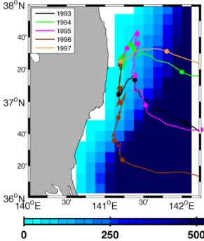
The vertical integral, from the seafloor to the surface, of the 137Cs activities yields a two-dimensional, horizontal distri-bution. A measure of the average horizontal position of the 137Cs patch is then given by the center of mass of the ver-tically integrated activities. This metric renders the compar-ison of various simulated137Cs patches in one figure possi-ble. Figure 9 shows that the “realistic” simulations (nominal years 1993 and 1996) feature a center of mass that is ini-tially southbound in accordance with what is expected from the state of the circulation as depicted in Fig. 6 and discussed in Sect. 3.2. Note that Fig. 9 carries also information about the simulated temporal variability of the cross-shelf trans-port: it takes the center of mass of the 1996 release more than 10 weeks to cross the shelf break (200 m isobath) south of 36◦N 40′. In contrast, the center of mass of the 1997 re-lease leaves the shelf way quicker, after less than a month, north of 37◦N 20′.
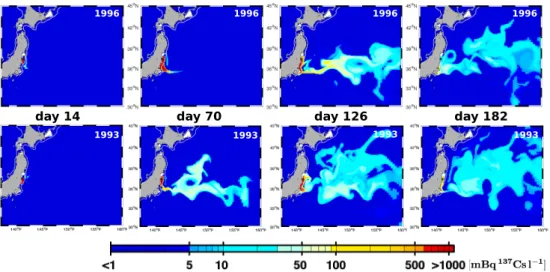
The further development of the “realistically” simulated (i.e. nominal years 1993 and 1996)137Cs patches is shown in Fig. 10. Three processes acting on137Cs leaving the shelf are apparent: (1) the Kuroshio accelerating137Cs eastwards into the basin; (2) mesoscale activity that disperses and mixes the 137Cs meridionally into the Kuroshio–Oyashio Interfrontal Zone where cold low salinity Oyashio water mixes with warmer high salinity Kuroshio water (Fig. 11); and (3) the near-coastal southward branch of the Tsugaru current that, together with the Oyashio current, flushes the east coasts of Honshu and Hokkaido north of 36◦N with uncontaminated waters originating from the Sea of Japan and the subpolar gyre, respectively.
Figure 10 also shows that even our “realistic” simulations differ considerably from one another. This holds especially for the appearance of enhanced (i.e. more than 10 mBq l−1) activities offshore east of 145◦E. But even though details
among the “realistic” simulations differ, common to all of them is that, ultimately, enhanced surface137Cs activities ap-pear in the Kuroshio–Oyashio Interfrontal Zone, a formation site of North Pacific Intermediate Water (NPIW) (Yasuda et al., 1995). Further, the simulations indicate that137Cs ac-tivities up to 4 mBq l−1prevail for more than a year in the re-gion (Fig. 12). This allows for enough time for the137Cs sig-nal to enter the NPIW before it is flushed away. Hence,137Cs discharged directly from the land to the sea off Fukushima may be a useful water mass tracer if its penetration into the NPIW can be measured in the years to come. Figure 13 pro-vides a model-based estimate of the137Cs concentrations in the NPIW, defined by its salinity minimum between 300 and 800 m, one year after the accident. Note that according to Park et al. (2008), they are above (although close to) the min-imum detectable activity (0.1 and 0.33 mBq l−1for deep and surface water, respectively).
5 Quantitative estimates of dilution
141oE 142oE 143oE
35oN
36oN
37oN
38oN
39oN
141oE 142oE 143oE
35oN
36oN
37oN
38oN
39oN
141oE 142oE 143oE
35oN
36oN
37oN
38oN
39oN
141oE 142oE 143oE
35oN
36oN
37oN
38oN
39oN
141oE 142oE 143oE
35oN
36oN
37oN
38oN
39oN
141oE 142oE 143oE
35oN
36oN
37oN
38oN
39oN
141oE 142oE 143oE
35oN
36oN
37oN
38oN
39oN
[m/s]
Obs. 7.4.2011
Obs. 12.3.1997
Mod. 7.4.1993 Mod. 7.4.1996
Mod. 7.4.1994 Mod. 7.4.1995 Mod. 7.4.1997
Fig. 6.Surface velocities at dates indicated by respective panel titles. The color shading denotes absolute velocity. The arrows indicate the
direction of the currents. The magenta line is the 200 m isobath, the red cross marks the nuclear power plant. The first column of panels (titled “Obs. 7.4.2011” and “Obs. 12.3.1997”) shows geostrophic velocities as estimated from space (Aviso, CNES). The subsequent panels titled “Mod. ...” refer to simulated currents. The upper and lower row of panels feature typical, contrasting states of the circulation, respectively (see text).
5.1 Horizontal diffusivity on the shelf
In the following, we will diagnose effective (model) diffu-sivities in our137Cs release simulations. The137Cs tracer is instantaneously released into one grid box. Intuitively, it is clear that the temporal evolution of both the maximum con-centration and the effective area occupied by the tracer car-ries the information to diagnose effective diffusivities. We find that the maximum concentration in the patch is not a good measure of diffusion in our model, because the steep gradients caused by the instantaneous point source give rise to numerical dispersion, until the gradients are smoothed out to some degree. As for the approach using a measure of the effective area, we follow Orre et al. (2008). We omit their derivation for the sake of brevity and merely document the calculations. The 137Cs tracer C(x, z, t ) is vertically inte-grated over the whole water column:
2(x, t )=
Z
C(x, z, t )dz. (2)
x(x, y)andzdenote the horizontal and vertical position, re-spectively.tis time. The vertical integral2(x, t )is normal-ized with the total (i.e. integrated over the entire model do-main) tracer content:
θ (x, t )= 2( x, t )
R
2(x, t )dx
. (3)
A measure of the effective area occupied by the tracer is de-fined by the second (physical space) moment of the vertically integrated and normalized tracer field:
µ2=
R
θ (x, t )|x−xcom(t )|2dx
R
θ (x, t )dx
, (4)
wherexcom(t )is the (horizontal) position of the center of mass of2(x, t ). An estimate of the effective diffusivityKis then given by
K=µ
2
4t. (5)
29 43 57 100
101 102
station 5 11
137
Cs [Bql
!
1]
29 43 57 100
101 102
station 6 12
29 43 57 100
101 102
station 7 1 2
29 43 57 100
101 102
station 8 3
137
Cs [Bql
!
1]
29 43 57 100
101 102
station 13
29 43 57 100
101 102
station 9 16
29 43 57 100 101 102 station 10 137 Cs [Bql ! 1]
days since 1!April
29 43 57 100
101 102
station 14
days since 1!April
29 43 57 100
101 102
station 17 20 19 18
days since 1!April
Fig. 7.Observed (red and blue o) by TEPCO and simulated (colored
lines) time series of surface137Cs activities at different stations as indicated by panel titles. The station numbers are assigned to loca-tions in Fig. 2. The black, green, magenta, brown, orange lines cor-respond to simulated nominal years 1993 to 1997, respectively. The grey lines correspond also to simulated year 1993 but with137Cs depositions being applied one week later. The blue o in the upper right panel denote measurements at stations 1 & 2, close to the dis-charge point.
are relatively similar among the ensemble members, are a consequence of numerical dispersion. With time (order of days), concentration gradients smooth out and the associ-ated numerical dispersion is suppressed as we enter the sad-dle phase. The length of the sadsad-dle phase is determined by the average movement of the tracer patch. As soon as a sig-nificant fraction of the tracer crosses the shelf-break and is gripped by the coastal southward branch of the Tsugaru cur-rent, the Kuroshio, or the vivid eddies offshore, the diffusiv-ity increases again. This explains why the saddle phase of the 1997 release, which reaches the shelf-break quickly (Fig. 9), is so much shorter than those of the other releases. We con-clude that the minimum values from 60 to 100 m2s−1 are representative for the diffusivity on the shelf.
5.2 Cross-shelf diffusivity
To obtain an estimate parameterizing, the cross-shelf ex-change as a Fickian diffusivity, the previous analysis is not helpful because it is unclear at what point in time (if at all) the above diagnosed diffusivity is representative of the cross-shelf exchange. A rough estimate can be obtained by apply-ing the diffusion equation
∂C ∂t =K
∂2C
∂x2, (6)
(whereCis the tracer concentration andKis the diffusivity) to a simple two box framework. One box resembles the shelf,
0 20 40
0 20 40 60
[S!1] [S!2] [A] [B]
137
)s +Bql
!
1/
0 20 40
0 10 20 30
[1] [2]
0 20 40
0 10 20 30 40
[9] [S!3]
0 20 40
0 20 40 60
[10] [S!4]
137
)s +Bql
!
1/
0 20 40
0 10 20 30 40 [3]
0 20 40
0 20 40 60
[4]
0 20 40
0 20 40 60 80 [5] [6]
days since 1!April
137
)s +Bql
!
1/
0 20 40
0 10 20 30 40 50 [7]
since 1!April
0 20 40
0 10 20 30 40 50 [8]
days since 1!April
Fig. 8.Observed (red o and vertical bars) by MEXT and
simu-lated (colored lines) time series of surface137Cs activities at dif-ferent stations as indicated by panel titles. The red vertical bars denote samples hosting137Cs activities below the detection limit (≈10 Bq l−1). The station numbers are assigned to locations in Fig. 2. The black, green, magenta, brown, orange lines correspond to simulated nominal years 1993 to 1997, respectively. The grey lines correspond also to simulated year 1993 but with137Cs depo-sitions being applied one week later. Note, that at station [4], day 14 a reading of 186 Bq l−1is not shown.
Fig. 9.Movement of the center of mass of simulated137Cs patches.
1996
1993
1996 1996 1996
1993 1993 1993
1993 day 70
day 14 day 126 day 182
Fig. 10.Simulated surface137Cs activities. Shaded in color is that fraction that is effected by the direct land-sea discharge. Background
activities present prior to the accident and effects of air–sea deposition are not accounted for. The upper and lower row of panels refer to simulations labeled by nominal years 1996 and 1993, respectively (also indicated in the upper right corner of each panel). The time information centered in each column of panels denote days elapsed since the137Cs discharge on 1 April of respective years. The 200 m isobath is indicated by white contours.
(a) (b)
Fig. 11.Simulated sea surface temperature and salinity on 1 April
of the nominal year 1993 (panel(a)and(b), respectively).
Fig. 12.Simulated (nominal year 1996 simulation) surface137Cs
concentration in units mBq l−1on 1 April, one year after the137Cs release off Fukushima Dai-ichi (indicated by the black x). Only ac-tivities, which according to Park et al. (2008), exceed the minimum detectable activity in surface waters, are shown.
33.1 33.6 33.8 34 34.2 34.4 34.6 34.8
20 N 25 N 30 N 35 N 40 N 45 N
0
200
400
600
800
1000
1200
Depth [m] 0.1
0.2 0.3
0.1 0.2
0.1
0.1
0.2
0.3
0.2
0.1
Fig. 13. Simulated (nominal year 1996 simulation) salinity (in
color) and137Cs activities (white contours) in units mBq l−1along 150◦E on 1 April, one year after the137Cs release.
the other the open ocean. Both have a spatial extent of1x. Assuming the concentration in the ocean box remains negli-gible compared to the concentration in the shelf box results in a spatial gradient determined solely by the concentration in the shelf box. The temporal evolution of the tracer concen-tration in the shelf box (Cs) is then determined by
∂Cs
∂t = − K
1x2Cs, (7)
which is solved by
Cs(t )=C0e−t τ
−1
0 10 20 30 40 50 60 70
102
103
Time [days]
Diffusivity [m
2/s]
1993 1994 1995 1996 1997
Fig. 14.Simulated diffusivity diagnosed (with Eq. 5) from the
effec-tive area covered by the released137Cs patch. Day zero corresponds to the time of release in the respective nominal years indicated by the figure legend.
with the initial concentrationC0and
τ=1x 2
K . (9)
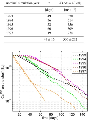
The timescale τ describes the rate of decrease of the total 137Cs content on the shelf. It can be interpreted as an effec-tive residence time of137Cs on the shelf as determined by the circulation. Figure 15 shows the decrease of simulated137Cs content on the shelf for the respective ensemble members: the content stays rather constant for several weeks, followed by a rapid decrease. The timing of the rapid decrease is cor-related with the center of mass approaching the shelf break (Fig. 9). Least square fitting of Eq. (8) applied to the first two months of rapid decrease shows reasonable skill (Fig. 15). The residence timescaleτ, averaged over all ensemble mem-bers is 43±16 days (Table 2). Assuming a shelf width,1x, of 40 km, this timescale corresponds to a horizontal diffu-sivity of 500±300 m2s−1. We interpret the uncertainty of ±300 m2s−1in the latter estimate as a measure of temporal variability.
6 Discussion
The rather realistic circulation is a real asset of our model (compare Sect. 3), especially because our simulations do not, in contrast to other studies (e.g. Qiao et al., 2011), fea-ture the long-time and almost endemic model problem of a Kuroshio separating from the coast too far north (Fig. 3). The agreement between observed and simulated137Cs ac-tivities (Figs. 7 and 8), however, might be misleading, either because we released an unrealistic amount of137Cs or be-cause our model misses a major mechanism removing137Cs activity from the surface ocean. To this end we discuss in the following so far unaccounted effects of (1)137Cs present in seawater already prior to the accident, (2) air–sea deposi-tion, (3) uncertainties of the direct land-sea discharge and (4) transfer of137Cs out of the water column into the sediment by137Cs adsorbed to settling biotic or abiotic particles.
1. Nakanishi et al. (2010) present 137Cs readings up to 4 mBq l−1in the waters of interest prior to the accident.
Table 2.Decay timescales (τ) derived from fitting Eq. (8) to
sim-ulated137Cs content on the shelf (Fig. 15). Diffusivities (K) are then calculated with Eq. (9) assuming a realistic shelf width (1x) of 40 km.
nominal simulation year τ K(1x=40 km)
[days] [m2s−1]
1993 49 378
1994 36 514
1995 52 356
1996 60 309
1997 19 974
43±16 506±272
20 40 60 80 100 120 140
1014 1015
time [days]
Cs
137
on the shelf [Bq]
1993 1994 1995 1996 1997
Fig. 15.Decline of the simulated 137Cs inventories on the shelf
(dashed lines). The time axis corresponds to days elapsed since the 137Cs was released in the nominal years indicated by the figure leg-end. The solid lines are least square fits to Eq. (8).
This offset has no significant effect on the agreement be-tween observed and simulated137Cs activities in Figs. 7 and 8. In contrast, it is a significant contribution to the simulated activities in Figs. 10, 12 and 13.
3. As pointed out already in Sect. 2.2, the amount of 137Cs discharged into the ocean is uncertain. Our simu-lations apply the IRSN (2011) estimate of 2.3 p Bq and (relatively insensitive to the timing of the discharge) are in reasonable agreement with observed activities as shown in Figs. 7 and 8. We realize that this as-sessment is subjective. The same would, however, ap-ply to more quantitative estimates of model-data mis-fit since they must contain some weighting of observa-tions, and this weighting, inescapably, is also subjec-tive to some extent. To summarize, we conclude based on Figs. 7 and 8 and the fact that simulated activities scale linearly with the total discharge that our simula-tions are consistent with observasimula-tions if the total dis-charge is within the envelope of the Japanese Gov-ernment (2011) (0.94 p Bq) and Tsumune et al. (2012) (3.5±0.7 p Bq). Our simulations are, however, appar-ently inconsistent with the high 27±15 p Bq estimate of Bailly du Bois et al. (2012) which we think is biased high: Bailly du Bois et al. (2012) extrapolate137Cs mea-surement in space and time to calculate weekly invento-ries contained by a 60×120 km box. Because the data is reasonably described by a logarithmic fit, they con-clude that an extrapolation backwards in time by one week to the anticipated time of discharge is admissible. Our criticism is threefold. First, their spatial extrapo-lation does not take into account that, initially, the cir-culation at the discharge location is southbound (which is also confirmed by Buesseler et al. (2011) based on 137Cs measurements). Hence, we expect low activities north, i.e. upstream of the nuclear power plant, whereas activities assigned by the “Point Kriging” applied by Bailly du Bois et al. (2012) assigns activities upstream, which rank among the highest in the whole region (their Fig. 4a). This biases their early inventories high. Sec-ond, their late (i.e. mid April till July) inventories are, on the other hand, biased low because of the detec-tion limit inherent to the respective137Cs measurements (10 to 50 Bq l−1, Buesseler et al., 2011). The detection limit may well transfer to a substantial inventory un-derestimation of 1 to 7 p Bq (in the 60×120 km box assuming a surface mixed layer depth of 20 m) but is not accounted for in the analysis. We conclude that the combined effect of “early” inventories biased high and “late” inventories biased low is an overestimation of the slope of the logarithmic fit that, by extrapolation back-wards in time, biases the discharge estimate of Bailly du Bois et al. (2012) high. Third, their extrapolation back-wards in time implicitly assumes a constant transport of 137Cs out of the box. This does not hold for the initial period after the discharge because, before leaving the box, the137Cs must first reach the box boundary. 4. Concerning the transfer of 137Cs to the sediment,
lessons learned in the Baltic Sea after the Chernobyl
ac-cident on 26 April 1986 give some guidance. As sum-marized in a short review in the associated paper in Ocean Science Discussions (Dietze and Kriest, 2011) (but discarded here for the sake of brevity), initially (i.e. on time scales of months to years), the redistribution of 137Cs should be dominated by physical processes such as mixing and advection.
In summary, our study seems to be consistent with available data and information (an exception being the Bailly du Bois et al. (2012) discharge estimate), but huge uncertainties re-main. Further, it cannot be used to produce any advise on hazards of radiative contaminants in general as it treats137Cs activities only. To this end it is noteworthy that elements like Pu are harder to detect at harmful concentrations.
7 Conclusions
We set out to quantify the mixing off Fukushima, Japan be-tween surface waters on the shelf and those offshore by simu-lating137Cs discharged in the aftermath of an accident at the nuclear power plant Dai-ichi on 11 March 2011. Our main tool was a global circulation model with an enhanced, eddy-resolving horizontal resolution in the region of interest. A comparison with sea surface height as observed from space and Argo float data showed that the model reasonably simu-lates actual conditions. This is supported by the model’s ca-pability of reproducing observed137Cs activities.
A caveat is the high uncertainty of the total 137Cs dis-charged directly from the land to the ocean. Obviously, if modeled 137Cs activities agree well with observation even though the simulated release is inconsistent with actual con-ditions, one ended up with getting the right answer for the wrong reason. Or in other words, as both the amount dis-charged and the circulation are uncertain to some degree, it is problematic to infer one from the other. What remains is to merely state that (1) we released 2.3 p Bq in our simulatrions following an estimate of IRSN (2011). This is, incidentally, almost exactly the average of the 0.94 p Bq estimate by the Japanese Government (2011) and the 3.5±0.7 p Bq estimate by Tsumune et al. (2012). (2) Our simulations are apparently inconsistent with the high 27±15 p Bq estimate of Bailly du Bois et al. (2012). (3) We think, as outlined in Sect. 6, that the latter estimate is biased high because of methodological issues.
the associated cross-shelf transport would necessitate a diffu-sivity of 500±300 m2s−1if applied on spatial scales similar to the actual shelf-width (40 km). The respective uncertain-ties are associated with the (simulated) temporal variability of the cross-shelf transport.
With respect to the fate of 137Cs discharged, our sim-ulations project enhanced surface activities offshore in the Kuroshio–Oyashio Interfrontal Zone which is known to be a formation site of North Pacific Intermediate Water (NPIW). Specifically, we find 10 to 50 mBq l−1six months after the release and an order of magnitude less after one year. This al-lows for enough time for a137Cs signal entering the NPIW. It is, however, close to the minimum detectable activity (MDA) in deep sea water (0.1 mBq l−1, Park et al., 2008). Note that the latter estimate refers only to the effect of the direct re-lease from the land to the ocean. Air–sea deposition of137Cs and background concentrations prior to the accident are not accounted for.
Acknowledgements. The constructive comments of two anony-mous reviewers and D. Tsumune helped to improve the manuscript. Discussions with C. B¨oning, U. Loeptien, A. Oschlies and I. Pisso are appreciated. GFDL is acknowledged for making MOM4 available. Computations were carried out on a NEC-SX9 at the University Kiel. Thanks to M. Collier at CSIRO for WOA 2005 conversion. The altimeter products were produced by Ssalto/Duacs and distributed by Aviso with support from Cnes. Argo data were collected and made freely available by the International Argo Program and the national programs that contribute to it (http://www.argo.ucsd.edu, http://argo.jcommops.org). The Argo Program is part of the Global Ocean Observing System. This work was supported by the SFB 754 of the German Research Foundation.
Edited by: M. Hoppema
References
Antonov, J. I., Locarnini, R. A., Boyer, T. P., Mishonov, A. V., Gar-cia, H. E., and Levitus, S.: World Ocean Atlas 2005, Volume 2: Salinity. NOAA Atlas NESDIS 62, U.S. Government Printing Office, Washington, DC, 182 pp., 2006.
Bailly du Bois, P., Laguionie, P., Boust, D., Korsakissok, I., Didier, D., and Fi´evet, B.: Estimation of marine source-term following Fukushima Dai-ichi accident, Journal of Environmental Radioac-tivity, doi:10.1016/j.jenvrad.2011.11.015, in press, 2012. Buesseler, K. O., Aoyama, M., and Fukasawa, M.: Impacts of
the Fukushima Nuclear Power Plants on marine radioactivity, Environ. Sci. Technol., 45, 9931–9935, doi:10.1021/es202816c, 2011.
Buesseler, K. O., Jayne, S. R., Fisher, N. S., Rypina, I. I., Bau-mann, H., BauBau-mann, Z., Breier, C. F., Douglass, E. M., George, J., Macdonald, A. M., Miyamoto, H., Nishikawa, J., Pike, S. M., and Yoshida, S: Fukushima-derived radionuclides in the ocean and biota off Japan, P. Natl. Acad. Sci. USA, 109, 5984–5988, doi:10.1073/pnas.1120794109, 2012.
Capet, X., Campos, E. J., and Pavia, A. M.: Submesoscale activ-ity over the Argentinian shelf, Geophys. Res. Lett., 35, 1–5, doi:10.1029/2008GL034736, 2008.
Dietze, H. and Kriest, I.: Tracer distribution in the Pacific Ocean following a release off Japan – what does an oceanic general circulation model tell us?, Ocean Sci. Discuss., 8, 1441–1466, doi:10.5194/osd-8-1441-2011, 2011.
Dietze, H., Matear, R. J., and Moore, T. J.: Nutrient supply to anti-cyclonic meso-scale eddies off western Australia estimated with artificial tracers released in a circulation model, Deep-Sea Res. I, 56, 1440–1448, doi:10.1016/j.dsr.2009.04.012, 2009.
Ducet, N. and LeTraon, P. Y.: A comparison of surface eddy ki-netic energy and Reynolds stresses in the Gulf Stream and the Kuroshio Current systems from merged TOPEX/Poseidon and ERS-1/2 altimetric data, J. Geophys. Res., 106, 16603–16622, 2001.
Fratantoni, D. M.: North Atlantic surface circulation during the 1990’s observed with satellite-tracked drifters, J. Geophys. Res., 106, 22067–22093, 2001.
Griffies, S. M., Gnanadesikan, A., Dixon, K. W., Dunne, J. P., Gerdes, R., Harrison, M. J., Rosati, A., Russell, J. L., Samuels, B. L., Spelman, M. J., Winton, M., and Zhang, R.: Formulation of an ocean model for global climate simulations, Ocean Sci., 1, 45–79, doi:10.5194/os-1-45-2005, 2005.
Griffies, S. M. and Hallberg, R. W.: Biharmonic friction with a Smagorinsky-like viscosity for use in large-scale eddy-permitting ocean models, Mon. Weather Rev., 128, 2935–2946, 2000.
Houghton, R. W., Hebert, D., and Prater, M.: Circulation and mixing at the New England shelfbreak front: Results of pur-poseful tracer experiments, Prog. Oceanogr., 70, 289–312, doi:10.1016/j.pocean.2006.05.001, 2006.
Institut de Radioprotection et de sˆuret´e nucl´eaire: Impact on the ma-rine environment of radioactive releases following the nuclear accident at Fukushima Dai-ichi 13th of May 2011, 2011. Japanese Government, Report of Japanese Government to the
IAEA ministerial conference on nuclear safety: The accident at TEPCO’s Fukushima nuclear power stations, Nuclear Emer-gence Response Headquaters, Government of Japan, 2011. Large, W. G., McWilliams, J. C., and Doney S. C.: Oceanic vertical
mixing: a review and a model with a nonlocal boundary layer parameterization, Rev. Geophys., 32, 363–403, 1994.
Ledwell, J. R., Watson, A. J., and Law, C. S.: Mixing of a tracer in the pycnocline, J. Geophys. Res., 103, 21499–21529, 1998. Liu, N., Eden, C., Dietze, H., Wu, D., and Lin, X.: Model-based
estimate of the heat budget in the East China Sea, J. Geophys. Res., 115, C08026, doi:10.1029/2009JC005869, 2010.
Locarnini, R. A., Mishonov, A. V., Antonov, J. I., Boyer, T. P., Gar-cia, H. E., and Levitus, S.: World Ocean Atlas 2005, Volume 1: Temperature, NOAA Atlas NESDIS 61, U.S. Government Print-ing Office, WashPrint-ington, DC, 182 pp., 2006.
Morino, Y., Ohara, T., and Nishizawa, M.: Atmospheric be-havior, deposition, and budget of radioactive materials from the Fukushima Daiichi nuclear power plant in March 2011, Geophys. Res. Lett., 38, L00G11, doi:10.1029/2011GL048689, 2011.
Jour-nal of RadioaJour-nalytical and Nuclear Chemistry, 283, 831–838, doi:10.1007/s10967-009-0422-y, 2010.
Niiler, P. P., Maximenko, N. A., Panteleev, G. G., Yama-gata, T., and Olson, D. B.: Near-surface dynamical struc-ture of the Kuroshio Extension, J. Geophys. Res., 108, 3193, doi:10.1029/2002JC001461, 2003.
Oke, P. R., Schiller, A., Griffin, D. A., and Brassington, G. B.: En-semble data assimilation for an eddy-resolving ocean model of the Australian region, Q. J. Roy. Meteorol. Soc., 131, 3301–3311, doi:10.1256/qj.05.95, 2005.
Okubo, A.: Oceanic diffusion diagrams, Deep-Sea Res., 18, 789– 802, 1971.
Orre, S., Gao, Y., Drange, H., and Deleersnijder, E.: Diagnos-ing ocean tracer transport from Sellafield and Dounreay by equivalent diffusion and age, Adv. Atmos. Sci., 25, 805–814, doi:10.1007/s00376-008-0805-y, 2008.
Park, J. H., Chang, B. U., Kim, Y. J, Seo, J. S., Choi, S. W., and Yun, J. Y.: Determination of low137Cs concentration in seawater using ammonium 12-molybdophosphate adsorption and chemi-cal separation method, J. Environ. Radioactivity, 99, 1815–1818, doi:10.1016/j.jenvrad.2008.07.006, 2008.
Qiao, F. L., Wang, G. S., Zhao, W., Zhao, J. C., Dai, D. J., Song, Y. J., and Song, Z. Y.: Predicting the spread of nuclear radiation from the damaged Fukushima Nuclear Power Plant, Chinese Sci-ence Bulletin, 56, 1890–1896, doi:10.1007/s11434-011-4513-0, 2011.
Stohl, A., Seibert, P., Wotawa, G., Arnold, D., Burkhart, J. F., Eck-hardt, S., Tapia, C., Vargas, A., and Yasunari, T. J.: Xenon-133 and caesium-137 releases into the atmosphere from the Fukushima Dai-ichi nuclear power plant: determination of the source term, atmospheric dispersion, and deposition, Atmos. Chem. Phys., 12, 2313–2343, doi:10.5194/acp-12-2313-2012, 2012.
Sundermeyer, M. A. and Price, J. F.: Lateral mixing and the North Atlantic Tracer Release Experiment: Observations and numeri-cal simulations of Lagrangian particles and a passive tracer, J. Geophys. Res., 103, 21481–21497, 1998.
Torgersen, T., DeAngelo, E., and O’Donnell, J.: Calculations of hor-izontal mixing rates using222Rn and the controls on hypoxia in Western Long Island Sound, Estuaries, 20, 328–345, 1997. Tsumune, T., Tsubono, T., Aoyama, M., and Hirose, K.:
Distri-bution of oceanic137Cs from the Fukushima Dai-ichi Nuclear Power Plant simulated numerically by a regional ocean model, J. Environ. Radioactivity, doi:10.1016/j.jenvrad.2011.10.007, in press, 2012.
Uchida, H., Imawaki, S., and Hu, J.-H.: Comparison of Kuroshio surface velocities derived from satellite altimeter and drifting buoy data, J. Oceanogr., 54, 115–122, 1998.
Uppala, S. M., Kallberg, P. W., Simmons, A. J., Andrae, U., Bech-told, V. D., Fiorino, M., Gibson, J. K., Haseler, J., Hernandez, A., Kelly, G. A., Li, X., Onogi, K., Saarinen, S., Sokka, N., Al-lan, R. P., Andersson, E., Arpe, K., Balmaseda, M. A., Beljaars, A. C. M., van de Berg, L., Bidlot, J., Bormann, N., Caires, S., Chevallier, F., Dethof, A., Dragosavac, M., Fisher, M., Fuentes, M., Hagemann, S., Holm, E., Hoskins, B. J., Isaksen, L., Janssen, P. A. E. M., Jenne, R., McNally, A. P., Mahfouf, J.-F., Mor-crette, J.-J., Rayner, N. A., Saunders, R. W., Simon, P., Sterl, A., Trenberth, K. E., Untch, A., Vasiljevic, D., Viterbo, P., and Woollen, J.: The ERA-40 re-analysis, Q. J. Roy. Meteorol. Soc., 131, 2961–3012, doi:10.1256/qj.04.176, 2005.
Yasuda, I., Okuda, K., and Shimizu, Y.: Distribution and modifica-tion of North Pacific Intermediate Water in the Kuroshio-Oyashio Interfrontal Zone, J. Phys. Oceanogr., 26, 448–465, 1995. Zhai, X. and Greatbatch, R. J.: Inferring the eddy-induced