AUTOMATIC LANDMARK RECOGNITION IN
AERIAL IMAGES USING ORB FOR AERIAL
AUTO-LOCALIZATION
Abstract—Aerial navigation based on computer vision is a subject in constant development, in terms of techniques and models, to identify the localization of the Unmanned Aerial Vehicle based on images. This paper employs the ORB algorithm in an application to identify landmarks, on a video obtained by an UAV. The ORB can be used to identify specific objects in a scene based on a reference image, through the analysis of the neighbourhood of keypoints, aiming at robustness under variations in rotation, brightness and translation, although it is not as strong in scale. Through the identification of those landmarks, which coordinates are previously well known, it is possible to develop algorithms to identify the aerial localization. Keywords-UAV; ORB; Computer Vision; Landmark recogni-tion.
I. INTRODUCTION
In the past few years, it has been observed an increase on the development of Unmanned Aerial Vehicles (UAV), not only due to the technological and computational development, but also due to the diverse applications, such as: urban areas and frontiers surveillance [refs]; object recognition [refs]; autonomous navigation; electrical transmission line inspection [?]; oil pipelines monitoring. The UAV, also known as Drone, has been used in both civil and military application. The UAV guidance system can be done in different ways: remotely con-trolled, autonomous or semiautonomous. Remotely controlled or semiautonomous UAVs require flight information capture, but the decision making is up to a pilot, who depends on his abilities and training. The usage of autonomous systems for navigation, on the other hand, is best fit when there are routine operation, or when they demand a high level of physical (duration of each operations) and mental efforts (obtaining flight information and data from the aircraft and the field) of the pilots. The navigation consists in obtaining information regarding the flight, the field and the aircraft itself. There are different systems that provide information for the navigation, such as the Inertial Navigation System (INS) and the Global Positioning System (GPS). Another solution for the navigation system would be through the employment of images and videos, captured by the UAV. The UAV position, therefore, influences on the captured scene, so it must be taken into consideration differences in rotation, scale and angle in the captured videos; the time of flight and also climate conditions are aspects that influence the scene captured; and also, depending on the sensor used, different videos, with different characteristics can be obtained. The videos obtained
by the UAV have to be processed in a embedded system. A. Related work
In [1], the SIFT algorithm is used to generate mosaic images, in automatic fashion, from other images obtained by the UAV. A non-linear optimization algorithm is used to estimate the position and attitude of the UAV. [2] describes a technique to determine the camera’s relative position and orientation to the UAV, from flight information (GPS and INS) and from the detection of a landmark with known geographical coordinates.
Some other methods related to Computer Vision are cited by [3], which aim at controlling an UAV autonomously. The techniques are corner detection for autonomous landing and autonomous refueling; Lukas-Kanade algorithm and the use of SIFT with Random Sample Consensus (RANSAC) for tracking; Wrapping Functions to find the relation between frames of the video; and particle filtering framework based on Bayesian network for aerial surveillance.
In [4], a particle filtering framework is used for the au-tonomous navigation of UAV. The UAV localization is de-termined by the analysis of two images captured in different moments, and used for stereo vision, and a Digital Elevation Model (DEM). A similar approach was proposed by [5], which presents autonomous navigation techniques using only a monocular camera and a DEM. Those techniques do not need GPS or INS.
In [6], the SIFT algorithm is used with an Extended Kalman Filter (EKF) to perform a SLAM. The result of the SLAM is used to determine the UAV localization, and build a 3D map of the field. The features triangulation is mentioned. [7] also presents a SLAM technique, using data from a LiDAR (Light Detection and Ranging) sensor, with the UAV camera.
The problem of UAV localization by means of features triangulation is addressed by [8]. Those features are detected using SIFT or SURF. It does not make use of GPS, but it depends on a previously obtained map of features. [9] uses an implementation of the SURF algorithm in a GPU and a geo-referenced image database to devise an autonomous navigation system without GPS.
Fig. 1. Block Diagram for feature-based Pattern Recognition.
and noises in images, which are common in aerial videos. The most important aspect, though, that led to its choice was the low processing burden required by ORB, which is an important asset for real-time applications.
II. AUTO-LOCALIZATION USINGIMAGES
Autonomous navigation of aircrafts and UAVs consists of a INS sensor, which informs its attitude, but, in a long term, this sensor accumulates errors. It is, then, necessary to have other sensors that will correct the INS. One way to do so is through the GPS, which auto-localizes the aircraft and corrects the INS. Other alternatives to correct the INS are studied, and one of them is by using Computer Vision and Image Processing algorithms, through images captured during flight.
[10] describes the Terrain-Aided Navigation (TAN) tech-nique to generate position information for the navigation, using visual-aided measures through the horizon profile. Another work [11] uses a camera and a gimbaled laser sensor to extract feature points from the environment that will be processed by an extended Kalman filter (EKF) in a SLAM. Using that same algorithm, [12] proposes a new method in the real-time inter-row tracking and localization technique.
In this article [13], the authors study the challenges to perform a collaborative navigation, including positioning, with multiples sensors in different agents. [14] develops a coop-erative multi-UAV, equipped with stereo vision cameras, to capture visual information that will be fused, in order to improve mainly aspects of robustness to noises in the SLAM algorithm.
[16] proposes a method to compute the UAV attitude and localization through ground landmarks, using the SIFT (Scale-Invariant Feature Transform) algorithm. The localization of the UAV is used to locate mobile ground targets.
III. METHODOLOGY A. The ORB Algorithm
As illustrated in Fig. 1, the ORB algorithm consists of three steps: keypoints localization, point descriptors computation and point descriptors match.
The keypoints localization has as input an image, and as output a set of points coordinates, where there are the charac-teristics that describes the input scene. How the keypoints are determined is based on an heuristic empirically chosen. For
that, the ORB uses an adapted version of the FAST algorithm, which detects corners in the image.
The computation of Point Descriptors has as input an image and the set of keypoints. For each keypoint, a neighbourhood of its coordinates is analyzed, calculating other descriptors for the region, related to its statistical aspects. For that, ORB uses an adapted version of the BRIEF algorithm, which does brightness variation tests on the region. This step produces as output a descriptor sequence of bits for each keypoint from the input.
The Point Descriptor’s matching has as input a set of reference descriptors and a set of test descriptors. Considering a descriptor as a point in the space of attributes, and its values (in this case, its bits) as its coordinates; for each reference descriptor, the algorithm will search for the closest point among the test descriptors. The output of this step is a set of pair of points(P, Q), whereP is a point in the reference image andQis a point in the test image. Each point is represented by their coordinatesxandy in the input image.
After the application of the ORB algorithm, a set of keypoints in the image is obtained and their supposed cor-responding position in the test image. For each pair of points, there also is the distance between them in the attribute space. The value of the distance is always an integer between 0 and 255 (including both), as it is calculated only by counting the different bits in a 256 sequence.
B. Calculating the Projection
The objective of this paper is to present a technique to detect the same object in distinct images, even if the point of view of the object is different in each image. In the case of aerial images, it is desired to identify the same targets, in spite of the aircraft’s new orientation, or height. Knowing the localization (geographical coordinates) of the previous record, it is desired to determine the position and orientation of the aircraft in flight, using the information gathered from the ORB.
this transformation can be obtained from three pair of points, as now, the mapping works in a 3D space.
Considering thestandard triangle, whose vertices are(1,0), (0,1) e (0,0). Given three points P, Q and R in R2, the mapping of the standard triangle on theP QRtriangle is given by the linear transformation in Eq. 1.
! ! ! ! ! ! x0 y0 1 ! ! ! ! ! !
= ! ! ! ! ! !
Px−Rx Py−Ry 0 Qx−Rx Qy−Ry 0
Rx Ry 1
! ! ! ! ! ! ! ! ! ! ! ! x y 1 ! ! ! ! ! !
(1)
Given two triangles ∆1 and ∆2, it is desired to determine the mapping between their coordinates. From Eq. 1, the matricesM1 andM2 are obtained, which permits to map the standard triangle on each∆1 and∆2, respectively. Using the operations of inversion and matrix multiplication, it is possible to obtain the matrixM, which gives the linear transformation that maps ∆1 on∆2, as it is in Eq. 2. Note thatM1−1 maps ∆1 on the standard triangle.
M =M−1
1 M2 (2)
Since ORB gives a setC of pair of points, as described in Eq. 3, it is possible to choose a subset ofC, with only 3 pairs, and determine the matrixM, that mapsPionQi,0<=i <3, using Eq. 1 and Eq. 2. However, there are no guarantees the pairs of points in Creally represent the same physical object captured in different images. In fact, if both input images are from completely different places, no pair in C will be valid. It is necessary to employ forms to filter the pair of keypoints given by the ORB, in order to remove all the false positive results.
C={(Pi, Qi)|0<=i < N;N"3} (3) C. Selection of pair of keypoints
In a set of pair of points, it is desired to find a subset of pairs, that can better represent the same physical object in two different images. In section III, to each pair, there is an associated distance for the descriptors in the attribute space. This distance indicates how similar the pair is, according to their descriptors. As the descriptors are extracted based on the pixels of the near neighbourhood of the keypoint, the distance in the attribute space does not take into consideration the relative position of the keypoints in the image. For example, houses in the same residential block may present similar characteristics in an aerial reference image. To localize one of those houses in another aerial image, it will not be enough to search for points with the most statistical similar pixel neighbourhood, from any small deviation in the data which can be caused by noises, luminosity differences, among other factors may result in a failed recognition, as the points that characterize the objects are too close in the attribute space.
IV. RESULTS
In this paper different case studies have been analysed. The algorithm developed has been applied in aerial images
captured by UAV flights. Different landmarks and flights were considered. In a first test, landmarks at ground level (Type I) were used: paintings on asphalt; tab street and manhole. In a second test, constructions (Type II) were considered. In a third test, the landmarks and their neighbourhood (Type III) were considered. Some landmarks of the video were selected as patterns to be recognized. These landmarks were employed due to the presence of corners.
The invariance in the object recognition was observed, especially when the image was rotated, as it is shown in Fig. 2.
Fig. 2. Pattern recognized in different angles of rotation.
The recognition of different patterns simultaneously was also tested. This approach may help in the auto localization, but also implies a higher computational cost. One of the results is shown in Fig. 3.
Fig. 3. Multiple patterns recognized simultaneously.
The algorithm’s sensitivity was calculated as the proportion of positive matches correctly identified. Similarly, the speci-ficity was calculated as the proportion of frames correctly identified as not containing the pattern. Both measures are shown in Table I.
V. CONCLUSION
TABLE I
STATISTICAL RESULTS FOR DIFFERENT LANDMARKS. Type Landmark Sensitivity Specificity
I 44% 98%
I 41% 90%
I 79% 98%
II 74% 89%
III 70% 90%
points were used as pairs of coordinates to define triangulation of landmarks. Different tests were performed. The identifi-cation of different landmarks have been tested. Furthermore, different flight situations were tested with variations in height, heading and attitude of the aircraft. The results indicate that the techniques can be used for identification of landmarks present in aerial images. In the analysis results, it can be seen that the identification of landmarks and their neighborhood improves the sensibility and the specifity. As future work, the application of techniques on images obtained at greater heights is proposed, in order to consider larger landmarks like Soccer fields, roads and airport runways. Furthermore, it is desired to implement in embedded systems.
REFERENCES
[1] T. Suzuki, Y. Amano, and T. Hashizume, “Vision based localization of a small uav for generating a large mosaic image,” 2010.
[2] A.-P. Hu, “Camera calibration for uav ground feature localization,” 2011. [3] Y.-C. Liu and Q.-H. Dai, “Vision aided unmanned aerial vehicle
auton-omy: An overview,” 2010.
[4] J. Zhang, W. Liu, and Y. Wu, “Novel technique for vision-based uav navigation,” 2011.
[5] Y. Kim, D. Lee, and H. Bang, “Vision-only uav navigation aided by terrain elevation map,” 2012.
[6] T. Suzuki, Y. Amano, and T. Hashizume, “Development of a sift based monocular ekf-slam algorithm for a small unmanned aerial vehicle,” 2011.
[7] C. Bodensteiner, W. Hbner, K. Jngling, P. Solbrig, and M. Arens, “Monocular camera trajectory optimization using lidar data,” 2011. [8] S. Rady, A. Kandil, and E. Badreddin, “A hybrid localization approach
for uav in gps denied areas,” 2011.
[9] X. Guan and H. Bai, “A gpu accelerated real-time self-contained visual navigation system for uavs,” 2012.
[10] S. Dumble and P. Gibbens, “Efficient terrain-aided visual horizon based attitude estimation and localization,” 2014.
[11] S. Huh, D. Shim, and J. Kim, “Integrated navigation system using camera and gimbaled laser scanner for indoor and outdoor autonomous flight of uavs,” 2013.
[12] N. Thamrin, N. Arshad, R. Adnan, R. Sam, N. Razak, M. Misnan, and S. Mahmud, “Simultaneous localization and mapping based real-time inter-row tree tracking technique for unmanned aerial vehicle,” 2012. [13] A. Kealy, G. Retscher, A. Hasnur-Rabiain, N. Alam, C. Toth, D.
Grejner-Brzezinska, T. Moore, C. Hill, V. Gikas, C. Hide, C. Danezis, L. Bonen-berg, and G. Roberts, “Collaborative navigation field trials with different sensor platforms,” 2013.
[14] X. Li and N. Aouf, “Experimental research on cooperative vslam for uavs,” 2013.
[15] L. Jayatilleke and N. Zhang, “Landmark-based localization for un-manned aerial vehicles,” 2013.
Real-Time Ray-Casting Volume Rendering using
GLSL
Marcos Araujo Polytechnic school - UFRJ
Rio de Janeiro, Brazil Email: [email protected]
Ricardo Marroquim COPPE - UFRJ Rio de Janeiro, Brazil Email: [email protected]
Fig. 1. Preview of our method’s results. Three different datasets rendered with three different transfer functions. The transfer function used for the lobster (middle) is also represented (inside the white box).
Abstract—Our work consists on the development of an appli-cation capable of real-time volume rendering. The main goal of this work is to boost the frame rates by taking full advantage of GPU shader programming with modern OpenGL and GLSL. GPU techniques are employed both for image composition and volume processing.
The application allows for interactive scalar volumetric datasets visualization with lighting and color using 2D transfer functions.
Keywords-volume rendering; ray casting; transfer functions; GLSL;
I. INTRODUCTION
In computer graphics a volume can be represented as a tridimensional matrix composed by voxels, which are anal-ogous to pixels in a bidimensional image. These datasets are generated by procedures such as computed tomographies (CT) magnetic resonance imaging (MRI), or simulations, like data obtained from computational fluid dynamics (CFD). Volumetric visualization is of major importance in fields like archeology, medicine and physics.
Rendering these volumes in the clearest way possible is important to allow a good understanding of the analyzed datasets and their characteristics. The goal of this project is
to provide a real-time rendering with illumination, as well as the option to use specific transfer functions.
The methods used for the application development are based on OpenGL4, and shader programming in GLSL using the ShaderLib Library [1]. This library is a wrapper for modern OpenGL programming, unburdening the developer from repet-itive setups and from tracking OpenGL’s state variables. The library also offers some utilities such as mesh loaders and a built in trackball system.
In Section II we present volume rendering concepts, and discuss the ray-casting method in Section III. Application results are presented in Section IV and we conclude the work in Section V.
II. VOLUMERENDERING
In our application domain, volume rendering consists in taking a scalar volumetric dataset and processing it to output intelligible images. The datasets are tridimensional voxel ma-trices, usually composed by 2D layers. The size of the layers and their spacing are dependent on the dataset.
of the scalar values. Given any chosen point in the volume’s space, its value can be determined by the trilinear interpolation of the point’s eight nearest neighbors. As we are working with 3D textures, this interpolation comes for free since it is directly supported by the graphics software.
There are many methods that can be used to render a volumetric dataset, some described in [2] and many analyzed in [3]. The method chosen for this project is the GPU-Based Ray Casting with local gradient-based illumination and color determination through transfer functions, very similar to the one presented in [4], except that our method uses transfer functions (Section III-D) to acquire color and opacity information. This kind of method is classified by the survey [3] as a local region-based technique, that, according to the paper, scales well with data and image size. Also, the same survey states that this type of application is sensitive to noisy data, as we can observe on the results presented in this paper(Section IV).
Also, in the field of medical visualization, [5] has imple-mented three volume rendering methods (ray-casting, splat-ting, shear-warp) and conducted a blind comparison of images rendered by them. The scientist-guided evaluation concluded that, of the three methods, ray-casting was the only acceptable for medical imaging due to flaws exhibited by the other two algorithms’ results.
Therefore, the method we implemented balances scalability, good image quality and low implementation complexity. There are some acceleration techniques for Ray-Casting [6] that are easy to implement, and significantly increases rendering per-formance without quality degradation. We have implemented one among these, more specifically, the early ray termination.
III. RAYCASTING
The GPU-Based Ray Casting method consists, in the case of an orthographic camera setup, in ”shooting” a parallel ray matrix through the volume, each ray being cast from one of the image’s pixels. Along each ray, the volume is sampled several times in different discrete positions, as if it was ”walking” with a fixed step size. See Figure 2 for an illustration of the method.
In our application pipeline, the first step is to set up the scene’s geometry (Section III-A), followed by the ray-sampling (Section III-B). In a pre-processing stage we cal-culate the gradient field (Section III-C). During ray-traversal we use transfer functions (Section III-D) to obtain RGBA values for the pixel color composition (Section III-E). We also employ illumination effects using the gradient vector (Section III-F).
A. Rendering space setup
The setup consists in representing the volume as a paral-lelepiped centered on the world space’s origin, the camera’s image plane, and a light source positioned in space. No vertex structure is created for the volume as our representation is implicit, since we only need to know the parallelepiped’s dimensions.
Fig. 2. Representation of the Ray Casting setup.
The plane is a square mesh, created as a simple mesh with four vertices, with the sides as large as the parallelepiped’s greater diagonal. Its distance from the world’s center is always half of this diagonal in order to avoid clippping the volume out of the viewport. This plane can be rotated around the volume using the trackball system implemented in the ShaderLib. B. Volume sampling
Volume sampling is executed during rendering in the frag-ment shader. As recommended in [2], the number of samples taken inside the volume is two times the number of voxels in the largest dimension of the volumetric dataset. For example, if the volume has dimensions (250,150,300), we sample the volume 600 times for each ray.
Each ray is cast from a pixel of the image plane. To sample the volume in a specific time step while traversing a given ray, we have to know what are the world coordinates for the pixel that generated the ray, the direction pointed by the rendering plane, and the step size.
With this information we first convert from pixel coordinates to the plane’s local coordinate system. Then, with the plane’s dimensions and it’s origin in world coordinates we calculate the pixel’s world position. Then, the steps are taken from the pixels in the direction of vˆd (depth vector, refer to
Figure 3), that points to the world’s origin. At each step, a four-component vector is sampled from the volume, containing a gradient vector (three components) and a scalar value. The whole proccess is carried out inside afragment shader. C. Gradient calculation
Fig. 3. The unit vectors in relation to the plane.
Fig. 4. Representation of a voxel and it’s six nearest neighbors.
Considering Figure 4 we compute the gradient vector for a voxel using its six nearest neighbors’ values, as follows:
~
grad= (v4, v3, v1)−(v2, v5, v6)
This operation is carried out inside a compute shader that dispatches one instance per voxel. It is executed during the application setup, so it computes the entire gradient field for the volume in a pre-processing stage.
In another compute shader, we smooth the gradient field by computing the mean vector between each voxel and its six neighbors. Refer to Figure 5 for a comparison between non-smoothed and smoothed gradient fields.
D. Transfer functions
The transfer function is a way to render the scalar volume into more elucidating images. In each sampled position the scalar value and the magnitude of the gradient vector are used to map from a two-dimensional matrix to a four-component vector. These components define a color (RGB) and an opacity value, which are the optical properties used to calculate the propagation of light inside the volume. Figure 6 depicts a 2d transfer function. In this case, we are considering absorption-only volumes, so no emission or scattering is taken into account.
Fig. 6. Example: transfer function mapping two parameters. The alpha channel is not represented in this image.
E. Color and gradient composition
Along each ray, the Ray Casting algorithm samples points inside the volume, acquiring a four component vector (voxelV alue~ ), where the first three components define the gradient vector, and the last is the scalar value. The gradient vector’s magnitude and the scalar value are used to map a RGBA vector (curV ector~ ) in a 2D transfer function. We define a scalar floating point value transp as the ray’s transparency (alpha channel). For each time step, we update the transparency value and compose the accumulated color (AcColor~ ) for each ray (therefore, each pixel) in the following manner:
transp=AcColor.A~ ~
AcColor=AcColor~ + (1.0−transp)×curV ector~
We also compose the gradient vector (AccGradient~ ), in order to use it during illumination calculations (described in the next subsection). The following update is realized if we have not yet saturated the gradient’s alpha channel:
~
Fig. 5. Comparing renderings with the original gradient field (left) and the smoothed one (right)
F. Illumination
For illumination effects we are using a simplified version of the Phong shader presented in [2]. We compute only the diffuse illumination component (dif f~ ) for each pixel based on the normalized vector composed of the accumulated gradient vectors (AccGradientˆ ), the light source position (LightP os~ ), and the accumulated color for the pixel (AcColor~ ). The diffuse component is then defined as follow:
~
dif f =AcColor~ ×max(LightP os~ ×AccGradient.xyz,ˆ 0.0)
IV. RESULTS
In Table I we present, for five different datasets, the av-erage time for pre-processing the gradients (computation and smoothing), and the frame rates presented by the application when rendering these volumes. These results were achieved on a GeForce GTX 770 GPU.
TABLE I
PRE-PROCESSING ANDRENDERING TIMINGS.
Data Dimensions (voxels) Grad (ms) FPS
neghip 64x64x64 12 667
lobster 301x324x56 121 158
engine 256x256x128 180 180
skull 256x256x256 354 158
foot 256x256x256 359 158
The following figures (7, 8, 9, 10, 11) represent some of the application’s results. The datasets were all downloaded from www.volvis.org.
The transfer function in Figure 8 was procedurally generated just as a simple sanity test for our implementation. On the other hand, the transfer functions used in figures 9 to 11 were crafted by trial and error in a image editing software to achieve the desired effect for each image.
As mentioned before, the method is sensitive to noisy data, as can be perceived in the results, specially the one in Figure 5.
V. CONCLUSION AND FUTURE WORKS
In this article we have presented real-time volume render-ing concepts, includrender-ing the use of two-dimensional transfer
Fig. 7. Rendered from the CT dataset of a foot, emphasizing the bones with the use of an adequate transfer function. Only the lightsource position has changed between the two images.
functions and pre-computed smoothed gradients. The results presented show the implementation of the Ray Casting tech-nique using modern GLSL and OpenGL techtech-niques is efficient and achieves interactive frame rates. The pre-processed gradi-ents are also carried out entirely in GPU, avoiding memory transfers, and thus implying in a very low setup overhead.
As future work, we are integrating our volume renderer with a method to compute the transfer-function semi-automatically through a few user interactions [7]. This integration will provide a more user-friendly way to navigate and investigate volumetric datasets in real-time. In addition, we would like to continue the path of exploring more complex real-time illumi-nation techniques for ray-casting using GPU programming.
REFERENCES
[1] V. de Andrade and R. Marroquim, “A shader library for opengl 4 and glsl 4.3 learning and development,” in Workshop of Undergraduate Works (WUW) in SIBGRAPI 2013 (XXVI Conference on Graphics, Patterns and Images), D. M. Maria Andreia Rodrigues, Ed., Arequipa, Peru, august 2013. [Online]. Available: http://www.ucsp.edu.pe/sibgrapi2013/ eproceedings/
[2] K. Engel, M. Hadwiger, J. M. Kniss, C. Rezk-Salama, and D. Weiskopf,
Real-time volume graphics, A. K. Peters, Ed., 2006.
Fig. 8. Example of an arbitrary transfer function in use to render two different volumes. The transfer function’s color are represented in the lower right corner, with no representation of the alpha channel.
Fig. 9. CT scan of two cylinders of an engine block (right) and the transfer function used for rendering(left).
Fig. 10. Rotational C-arm x-ray scan of phantom of a human skull (right) and the transfer function used for rendering (left)
Computer Graphics Forum, vol. 33, no. 1, pp. 27–51, 2014. [Online]. Available: http://dx.doi.org/10.1111/cgf.12252
[4] M. Levoy, “Display of surfaces from volume data,” IEEE Comput. Graph. Appl., vol. 8, no. 3, pp. 29–37, May 1988. [Online]. Available: http://dx.doi.org/10.1109/38.511
[5] M. Smelyanskiy, D. Holmes, J. Chhugani, A. Larson, D. M. Carmean, D. Hanson, P. Dubey, K. Augustine, D. Kim, A. Kyker, V. W. Lee, A. D. Nguyen, L. Seiler, and R. Robb, “Mapping high-fidelity volume rendering for medical imaging to cpu, gpu and many-core architectures,” IEEE Transactions on Visualization and Computer Graphics, vol. 15, no. 6, pp. 1563–1570, Nov. 2009. [Online]. Available: http://dx.doi.org/10.1109/TVCG.2009.164
[6] J. Kruger and R. Westermann, “Acceleration techniques for gpu-based volume rendering,” inProceedings of the 14th IEEE Visualization 2003 (VIS’03), ser. VIS ’03. Washington, DC, USA: IEEE Computer Society, 2003, pp. 38–. [Online]. Available: http://dx.doi.org/10.1109/VIS.2003.
10001
Um Modelo de Coordenação Extensível para
Múltiplas Visões Coordenadas
Rodrigo Stuani Brigatto, Danilo Medeiros Eler Unesp, Univ. Estadual Paulista
Faculdade de Ciências e Tecnologia de Presidente Prudente Departamento de Matemática e Computação [email protected], [email protected]
Resumo—Coordenação é um valioso mecanismo empregado em tarefas exploratórias em sistemas de múltiplas visões, uma vez que permite a rápida associação entre diferentes representações de um mesmo item em visões distintas. Embora existam vários modelos formais de coordenação, a maioria dos sistemas de múl-tiplas visões coordenadas (Coordinated Multiple Views – CMV) não emprega modelos formais. Isso provavelmente ocorre porque esses sistemas não precisam de mecanismos de coordenação mais complexos para auxiliar tarefas exploratórias, ou a extensão dos modelos existentes é muito trabalhosa. Neste documento, nós propomos um novo modelo de coordenação para simplificar a definição e a implementação de técnicas de coordenação; e a integração entre diferentes técnicas de visualização extraídas de diferentes sistemas de visualização. Este modelo foca somente no mecanismo de coordenação ao invés de questões de ma-nipulação do sistema não relacionadas à coordenação. Na sua primeira avaliação, o modelo proposto foi utilizado para definir e implementar técnicas de coordenação distintas encontradas na ferramenta Projection Explorer (PEx), na qual as técnicas de coordenação criam relações entre itens baseadas em ID, tópico e distância (similaridade).
Keywords-visualização; Múltiplas Visões Coordenadas; Modelo de Coordenação
Abstract—Coordination is a valuable interaction mechanism employed in exploratory tasks in multiple views visualization systems since it allows the fast association among different item representations from distinct views. Even though there are several formal coordination models, most coordinated multiple views (CMV) systems do not employ formal models. It probably occurs because these systems do not need more complex coordination mechanisms to aid in exploratory tasks, or the extension of existing CMV models is too laborious. In this paper we propose a new coordination model to simplify the definition and the implementation of coordination techniques; and the integration among distinct visualization techniques extracted from different visualization systems. This model focus only on the coordination mechanism instead of handling issues of the system that do not concern to the coordination. In its first evaluation, the proposed model was used to define and implement distinct coordination techniques found in Projection Explorer (PEx) tool, whose coordination techniques can create item relations based on ID, topic and distance (similarity).
Keywords-Visualization; Coordinated Multiple Views; Coordi-nation Model
I. INTRODUÇÃO
Múltiplas visões em visualização de informações é uma valiosa abordagem para a análise de dados. Ferramentas que
empregam tal abordagem implementam um conjunto de técni-cas de visualização que permitem ao usuário analisar conjuntos de dados sob diferentes perspectivas. Os usuários podem assim propor e avaliar hipóteses, e/ou descobrir padrões ou tendências nos dados. Além disso, uma das muitas vantagens dessa abordagem é que as limitações de uma técnica podem ser superadas por outra(s) técnica(s) [1]. Não obstante, pode ser difícil seguir ou fazer uma relação de itens de interesse sob diferentes representações visuais. A troca de contexto entre múltiplas visões pode prejudicar os benefícios do uso de múl-tiplas visões. Portanto, mecanismos de coordenação podem ser adicionados ao sistema de modo a solucionar este problema e tornar o processo exploratório mais efetivo. Estes mecanismos permitem a associação entre diferentes representações de um item e ainda facilitam a capacidade do usuário de encontrar relacionamentos que poderiam ser difíceis de reconhecer [2]. Coordenação entre diferentes visões geralmente é feita por meio de uma solução customizada ao invés de um modelo de coordenação genérico. Isso faz a implementação de técnicas de coordenação mais difícil uma vez que seus elementos específicos ou o fluxo de dados pode não ser bem definido e claro aos desenvolvedores. Geralmente, a maioria dos sistemas não emprega um modelo de coordenação porque eles somente utilizam técnicas de coordenação cujo mapeamento entre visões é computado baseado em identificadores de instância (IDs), no qual as mesmas instâncias selecionadas na visão de origem são destacadas nas outras visões. Entretanto, esta coordenação baseada em identificador pode limitar e dificultar a exploração de conjunto de dados distintos em um mesmo processo exploratório, limitando a capacidade do usuário de encontrar padrões e relações em conjuntos de dados mais complexos ou não relacionados. Além disso, quando um modelo formal não é empregado, a integração de técnicas de coordenação e visualização de outros sistemas ou modelos é muito trabalhosa porque a técnica de coordenação implantada em tal sistema precisa ser modificada para ser implantada ou para comunicar com outros modelos de dados.
poderiam ser propostas para estabelecer diferentes mapeamen-tos entre múltiplas visões e como integrar a arquitetura de sistemas distintos. Além disso, eles não fornecem mecanismos para permitir às técnicas de coordenação lidar com modelos de dados distintos, por exemplo, modelo de dados diferente do modelo relacional. Em resumo, as técnicas de coordenação e visualização têm de se adaptar ao modelo e não o modelo às técnicas existentes.
Este trabalho apresenta um novo modelo para coordenar múltiplas visões, o qual permite extensões de técnicas de coor-denação e sua integração com modelos de dados e arquiteturas de diferentes sistemas de visualização. O modelo proposto utiliza padrões de projeto [9] para fornecer uma solução formal genérica para definir os elementos, a informação requisitada, e o fluxo de dados para cada técnica de coordenação para auxiliar desenvolvedores a focar somente na própria coorde-nação ao invés de se preocupar com sua integração como o sistema-alvo. Ferramentas de visualização que adotam este novo modelo podem aumentar sua manutenibilidade, que é um importante fator de qualidade de um software [10], uma vez que facilita a tarefa de definir, adaptar, integrar e imple-mentar técnicas de coordenação no sistema. Além do mais, o modelo proposto supera algumas limitações dos modelos de coordenação existentes; permite a definição de técnicas de coordenação distintas para manipular diferentes tipos de dados, permitindo a exploração de conjuntos de dados distintos; e auxilia a parametrização do processo de exploração bem como os mapeamentos computados.
Este documento também apresenta a avaliação preliminar do modelo, apresentando como ele foi integrado na arquitetura da Projection Explorer (PEx) [11], uma ferramenta que fornece maneiras interessantes de desenvolver técnicas de coordena-ção para lidar com conjuntos de dados distintos no mesmo processo exploratório e que serviu de base para o modelo atual [6]. Assim, duas técnicas de coordenação diferentes foram implementadas utilizando o modelo e integradas com a PEx.
Este documento é organizado da seguinte maneira: o modelo é descrito na Seção 2. Aplicações do modelo proposto para demonstrar como instanciar técnicas de coordenação distintas e como integrar técnicas de visualização de diferentes sistemas são apresentadas na Seção 3. Conclusões e planos futuros são discutidos na Seção 4.
II. OMODELO
Este trabalho propõe um modelo que permite o desenvol-vimento de técnicas de coordenação distintas. Assim, cada técnica de coordenação pode manipular dados de diferentes conjuntos e computar tipos distintos de mapeamentos. Esta característica permite a exploração de diferentes conjuntos de dados no mesmo processo exploratório. Adicionalmente, nosso modelo permite a configuração de uma técnica de coordenação durante o processo exploratório. Portanto, o usuário pode configurar a maneira como o mapeamento será computado. Além do mais, nós permitimos o desenvolvimento de técnicas
de coordenação cujos mapeamentos são configurados durante a interação do usuário ou de acordo com a seleção do usuário. No modelo proposto, os mapeamentos podem ser estáticos ou dinâmicos. O primeiro ocorre quando o mapeamento é sempre o mesmo durante todo o processo exploratório, como em uma técnica de coordenação cujos mapeamentos são computados com base nos identificadores da instância (IDs), por exemplo. O último ocorre quando os elementos de dados empregados para sua computação podem variar de acordo com a interação do usuário, como em uma técnica de coordenação cujos mapeamentos são computados com base nos termos mais frequentes adquiridos das instâncias selecionadas, por exemplo. Um diagrama UML para o modelo proposto é apresentado na Figura 1. Uma breve descrição de cada classe e sua função no modelo é apresentado a seguir:
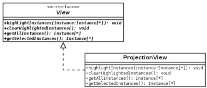
• ModelFacade: esta classe desempenha o papel da fachada do nosso modelo – engloba todas as outras classes do modelo e fornece um ponto único de acesso ao subsistema de coordenação;
• ModelFactory: esta classe tem a tarefa de criar objetos de coordenação com base no tipo de coordenação. Uma ins-tância desta classe deve ser fornecida à classe ModelFa-cade, de modo a fazer o modelo funcionar corretamente; • View: esta interface representa as visões que serão coor-denadas por meio do modelo. As classes das visões do sistema devem implementar esta interface, de modo que o nosso modelo possa se comunicar com o sistema; • Coordinator: esta é a classe principal do modelo. Ela
gerencia as coordenações associadas com cada visão de destino e transmite mensagens de coordenação para as visões associadas;
• Instance: esta interface deve ser implementada pela classe dos itens das visões sendo coordenadas pelo modelo. Ela é necessária para criar o correto mapeamento e para permitir a comunicação entre o modelo e o sistema; • Mapping: esta classe armazena os itens mapeados entre
visões. Para cada item na visão de origem, esta classe tem instâncias mapeadas na visão de destino;
• CoordinationList: esta classe armazena as coordenações relacionadas a uma visão de destino bem como a co-ordenação ativa para a visão de destino. Cada visão de destino para alguma coordenação tem sua própria lista de coordenações;
• Coordination: esta classe abstrata realiza e armazena os mapeamentos entre itens de duas visões. Ela contém a visão de origem e destino da coordenação e os mapea-mentos configurados pela técnica de coordenação; • StaticMappingCoordination: esta classe abstrata
repre-senta o grupo de técnicas de coordenação cujo mape-amento dos itens é criado no momento de criação da coordenação e permanece inalterado durante o tempo de vida da coordenação;
Figura 1. Diagrama UML para o modelo
o usuário e pode mudar durante o tempo de vida da coordenação;
• CoordinationParameter: esta classe armazena parâmetros necessários por algumas técnicas de coordenação. Por exemplo, se uma técnica de coordenação precisa saber quantos itens serão associados na visão de destino, é necessário armazenar esta informação em um objeto desta classe;
• ParameterView: esta interface é maneira através da qual algumas técnicas de coordenação podem fornecer parâ-metros ao sistema. O desenvolvedor deve implementar esta interface para cada técnica de coordenação que necessita de parâmetros;
• CoordinationType: esta classe é responsável por arma-zenar a técnica de coordenação para cada coordenação durante a execução bem como armazenar todas as téc-nicas de coordenação disponíveis para o sistema usando nosso modelo.
Nós adotamos duas perspectivas para descrever o modelo: uma do desenvolvedor interessado em usar nosso modelo para realizar a coordenação em um sistema de múltiplas visões e outra do desenvolvedor de técnicas de coordenação, interessado em criar (ou implementar) uma técnica de coor-denação usando nosso modelo. A próxima seção apresenta a instanciação do modelo sob essas duas perspectivas, tomando como base a ferramentaProjection Explorer (PEx) [11].
III. APLICAÇÃO
Esta seção apresenta aplicações do modelo proposto para implementar duas técnicas de coordenação da literatura e como elas foram incluídas na PEx. Por falta de espaço, a coorde-nação baseada em identificadores (IDs) não será apresentada. Os conjuntos de dados usados nas aplicações são coleções de documentos que contém resumos, nome de autores, título do
trabalho, palavras-chave e data de publicação.
A. Coordenação baseada em tópico
A técnica de coordenação baseada em tópico realiza o mapeamento baseado no tópico extraído das instâncias se-lecionadas [12]. Sempre que há uma seleção de itens na visão de origem, um tópico é gerado e os itens na visão de destino que são cobertos por este tópico são selecionados. A implementação atual desta técnica naPExconsidera o tópico no qual os termos têm maior valores de covariância.
A primeira tarefa aqui é definir qual informação é necessá-ria para realizar a coordenação. Uma vez que coordenação baseada em tópico precisa do conteúdo textual do arquivo para extrair os termos, nós estendemos a interface Instance definindo um método chamado getTextContent que retorna o conteúdo textual bruto do documento como uma string. É necessário computar o modelo de espaço vetorial e valores de covariância. Também, esta coordenação requer o nome do texto para identificar cada documento; portanto, outro método chamadogetTextName(que também retorna umastring) é adi-cionado. A classe resultante (que estende a interfaceInstance) é mostrada na Figura 2.
A próxima etapa é definir a classe da coordenação. Esta téc-nica de coordenação cria o tópico para cada seleção do usuário na visão de origem e determina quais itens serão destacados na visão de destino baseado neste tópico. Portanto, a classe da coordenação tem que estenderDynamicMappingCoordination, porque o mapeamento é dinâmico, uma vez que muda a cada interação/seleção do usuário.
A coordenação baseada em tópico realiza um pré-processamento no conjunto de dados, visto que ela tem que extrair o conteúdo textual bruto dos itens, eliminarstopwords, computar o modelo de espaço vetorial e, finalmente, o tópico. De fato, a maior parte do trabalho é realizada nesta etapa. Por este motivo, nós sobrescrevemos o métodopreprocessData da classe abstrataCoordination. Também é necessário definir um método auxiliar chamadocreateQueryScalar, para auxiliar na tarefa de identificar quais instâncias da visão destino são cobertas pelo tópico.
Finalmente, nós implementamos os métodos abstratos defi-nidos na classe Coordination: createMapping e relayMappe-dInstances. A classe resultante juntamente com sua hierarquia é mostrada na Figura 3.
Figura 3. ClasseTopicCoordinatione sua hierarquia
Esta técnica não precisa de parâmetros, então não é neces-sário criar uma classe para implementar a interface Parame-terView.
B. Coordenação baseada em distância
A coordenação baseada em distância realiza a associação doskvizinhos mais próximos na visão de destino baseada na computação similaridade (ou distância) [12]. Nesta técnica, o númeroké um parâmetro para a coordenação. Neste contexto, quanto mais próximo um item está de outro no espaço de características original, mais similar ele é àquele item.
Como a coordenação baseada em tópico, esta técnica de coordenação é bastante complexa, de modo que nós daremos uma visão superficial do processo, comentando detalhes so-mente quando relacionados ao modelo.
Seguindo nosso modelo, a primeira etapa é definir qual informação dos itens é necessária para realizar a coordenação. Como a coordenação baseada em tópico, esta técnica precisa do conteúdo textual bruto de cada item; por esta razão nós definimos um método para obter tal informação, chamado getTextContent, que retorna uma string Java com o texto representado por aquele item. Este método é empregado para fornecer uma informação textual para computar o modelo de espaço vetorial da coleção de documentos envolvidos no processo exploratório. Para isso nós definimos um método
chamado getTextName, que retorna o nome do texto sendo representado pelo item. A interfaceDistanceInstancepode ser vista na Figura 4. Alternativamente, em trabalhos futuros, nós poderíamos construir uma coordenação baseada em distância mais geral para obter um vetor de características dos itens ao invés do conteúdo textual. Assim, poderíamos utilizar esta técnica para coordenar qualquer tipo de conjunto de dados descrito por um espaço de características (e.g. coleções de imagens).
Figura 4. InterfaceDistanceInstanceestendendo a interfaceInstance
A próxima etapa é definir a classe de coordenação. Este tipo de coordenação realiza um mapeamento estático entre itens porque a associação entre cada item da visão de origem e os itens que são mais similares na visão de destino é definida no momento de criação da coordenação. Não importa quantos ou quais itens são selecionados na visão de destino, as instâncias mapeadas já estão definidas. Por esta razão, a classe DistanceCoordinationestende a classe abstrata Static-MappingCoordination.
Um pré-processamento é necessário por esta técnica de co-ordenação, então ela sobrescreve o métodopreprocessDatada classeCoordination. Este método realiza o pré-processamento dos modelos de espaço vetorial computados, de modo que eles tenham os mesmos atributos (termos). O resultado da etapa de pré-processamento é um novo espaço contendo os atributos comuns de ambas as visões. É necessário facilitar a computação da similaridade entre itens de visões distintas (modelos de espaço vetorial).
Além de fornecer implementar para os métodos create-Mapping e relayMappedInstances da classe Coordination, nós definimos alguns métodos auxiliares e atributos para a classeDistanceCoordination. A classe tem dois atributos para armazenar o novo espaço de atributos das visões de origem e destino (newSourcePoints e newTargetPoints, respectiva-mente). Os métodos definidos sãoaddDistance, que adiciona uma distância/similaridade computada para um novo par de elementos; transformMatrix, que realizar a transformação no modelo de espaço vetorial de acordo com o tipo selecionado de transformação; efindCommonNgrams, que encontra os termos comuns entre os dois conjuntos de documentos.
Figura 5. ClasseDistanceCoordinatione sua hierarquia
usada para reduzir o número de palavras sendo analisado baseado no stem ou radical das palavras), os cortes inferior e superior de frequência de termos e o tipo de transformação na matriz termo×documento. Os parâmetros requeridos uma vez são: a medida de similaridade entre itens (e.g. Euclideana, City Block ou distância do cosseno) e o número de itens a serem destacados na visão de destino (i.e. oskvizinhos mais próximos).
Seguindo as recomendações do nosso modelo para criar uma janela para obter os parâmetros dos usuários, nós definimos a classeDistanceParameterView. Esta classe estende a conhe-cida classe JDialoge implementa a interfaceParameterView. A superclasse JDialog já possui seu próprio método show; por isso, nós somente temos que implementar os métodos closeegetParametersdefinidos na interfaceParameterView. A Figura 6 apresenta o diagrama UML para a classe resultante – devido a restrições de espaço, a maioria dos atributos da classeDistanceParameterView foram suprimidos.
Figura 6. Diagrama UML para a classe DistanceParameterView, que implementa a interfaceParameterView
C. Integração com a Projection Explorer
Somente algumas mudanças foram necessárias para integrar o modelo e as duas técnicas de coordenação descritas nas subseções anteriores à ferramenta PEx. Como a ferramenta tem uma estrutura bem organizada e cada uma de suas classes tem um papel bem definido no sistema, a integração foi uma questão de encontrar quais classes desempenhavam o papel requerido pelo modelo.
Primeiramente, é necessário fazer com que a classe que representa as visualizações no sistema implemente a interface Viewdefinida pelo modelo. Na PExessa classe é Projection-View. A Figura 7 mostra a realização da interfaceView(devido a restrições de espaço, os outros métodos e atributos da classe ProjectionView foram omitidos).
Figura 7. Realização da interfaceViewpela classeProjectionView
Então, o modelo requer que, para cada técnica de coordena-ção, sua interface (a qual estende a interfaceInstance) deve ser implementada pela classe que armazena os itens da visualiza-ção. A classe que representa os itens de uma visualização na PExé a classeVertex. Uma vez que as técnicas de coordenação baseada em tópico e distância requerem a mesma interface, somente uma única implementação é necessária. A Figura 8 mostra a realização das duas interfaces pela classe Vertex (novamente, devido a restrições de espaço, nós omitiremos os atributos e outros métodos da classeVertex).
Figura 8. Realização das interfaces para as técnicas de coordenação por distância e tópico pela classeVertex
Agora, nós definimos a classe “fábrica” para o modelo (classe que estende a classe abstrata ModelFactory), imple-mentando os métodos abstratos definidos. No método create-Coordination a subclasse adequada deCoordination é criada baseada no parâmetrotype, o qual contém o nome da técnica de coordenação. O método createParameterView retorna as interfaces anteriormente descritas para obter parâmetros de coordenação do usuário (para a coordenação baseada em tópico, que não requer parâmetros, uma referência Java null é retornada). O método needParameters retorna um valor booleano verdadeiro para a técnica de coordenação baseada em distância e falso caso contrário. Finalmente, o método hasStaticMapping retorna o valor booleano verdadeiro para a técnica de coordenação baseada em distância e falso caso contrário.
Figura 9. ClassePExFactory, estendendo a classe abstrataModelFactory
A ação final foi passar uma instância daPExFactoryà classe ModelFacade(através do métodosetFactory) antes de começar a utilizar o modelo.
A Figura 10 apresenta um exemplo da técnica de coordena-ção baseada em distância. Nesse exemplo o usuário selecionou um grupo de documentos na visão origem e os cinco vizinhos mais próximos de cada documento foram destacados na visão destino. Os documentos selecionados e os destacados são aqueles cujo círculo está em negrito. A visão origem representa um conjunto de documentos da conferência IEEE InfoVis e a visão destino representa um conjunto de documentos da conferência Information Visualization. Por falta de espaço, não apresentaremos um exemplo de aplicação da técnica de coordenação baseada em tópico.
Figura 10. Coordenação baseada em distância naPEx
IV. CONCLUSÃO
Para um sistema de múltiplas visões coordenadas, o nosso modelo se mostra uma solução simples para realizar a coor-denação. A interface mínima estabelecida pelo modelo requer poucas mudanças no sistema (somente a implementação de algumas interfaces), uma vez que somente a informação ne-cessária para realizar a coordenação precisa ser fornecida.
O modelo proposto tem como objetivos o reuso e facilidade de uso. As técnicas de coordenação criadas usando o modelo podem ser utilizadas em qualquer sistema que também utiliza o modelo, sem qualquer modificação, levando ao reuso. O esforço e o tempo para o desenvolvimento de uma técnica de coordenação usando o modelo também são reduzidos. Somente
poucos requisitos são necessários para criar uma coordenação usando o modelo, uma vez que este consiste de um pequeno conjunto de classes das quais poucas precisam ser estendidas para alcançar o objetivo.
Uma técnica de coordenação definida por meio do modelo está encapsulada e é independente do sistema no qual é empregada. Além disso, o modelo permite criar diferentes coordenações usando diferentes configurações de parâmetros, proporcionando uma melhor exploração visual do conjunto de dados.
A implementação de técnicas de coordenação para a ferra-mentaProjection Explorermostrou que o modelo apresentado atende aos requisitos propostos. Em trabalhos futuros preten-demos validar nosso modelo com a integração com diferentes sistemas de visualização para assegurar que o modelo está completo, independente e coerente.
AGRADECIMENTOS
Os autores agradecem o apoio financeiro da Fundação de Amparo à Pesquisa do Estado de São Paulo (FAPESP) – Processo 12/22264-7.
REFERÊNCIAS
[1] D. A. Keim, “Information visualization and visual data mining,”IEEE Transactions on Visualization and Computer Graphics, vol. 8, no. 1, pp. 1–8, Jan. 2002.
[2] H. Chen, “Towards design patterns for dynamic analytical data visuali-zation,” inProceedings Of SPIE Visualization and Data Analysis, 2004, pp. 75–86.
[3] C. North and B. Shneiderman, “Snap-together visualization: Coordina-ting multiple views to explore information,” University of Maryland Computer Science, Tech. Rep., 1999.
[4] N. Boukhelifa, J. C. Roberts, P. J. Roberts, and P. J. Rodgers, “A coordi-nation model for exploratory multi-view visualization,” inProceedings of the conference on Coordinated and Multiple Views In Exploratory Visualization, ser. CMV ’03. Washington, DC, USA: IEEE Computer Society, 2003, pp. 76–.
[5] C. Weaver, “Building highly-coordinated visualizations in improvise,” in Proceedings of the IEEE Symposium on Information Visualization, ser. INFOVIS ’04. Washington, DC, USA: IEEE Computer Society, 2004, pp. 159–166.
[6] D. M. Eler, “Mltiplas vises coordenadas para explora de mapas de similaridade,” Ph.D. dissertation, Instituto de Ciias Matemcas e de Computa, Universidade de Saulo, Abril 2011.
[7] M. Sanver and L. Yang, “A linking mechanism to integrate components of a visualization framework,” in 13th International Conference on Information Visualisation, IV 2009, 15-17 July 2009, Barcelona, Spain. IEEE Computer Society, 2009, pp. 92–97.
[8] A. Heijs, “Requirements for coordinated multiple view visualization sys-tems for industrial applications,” inProceedings of the 11th International Conference Information Visualisation (IV ’07). Washington, DC, USA: IEEE Computer Society, 2007, pp. 76–79.
[9] E. Gamma, R. Helm, R. Johnson, and J. Vlissides, Design Patterns: Elements of Reusable Object-oriented Software. Boston, MA, USA: Addison-Wesley Longman Publishing Co., Inc., 1995.
[10] ISO/IEC, ISO/IEC 9126. Software engineering – Product quality. ISO/IEC, 2001.
[11] F. V. Paulovich, M. C. F. Oliveira, and R. Minghim, “The projection explorer: A flexible tool for projection-based multidimensional visua-lization,” inProceedings of the XX Brazilian Symposium on Computer Graphics and Image Processing, ser. SIBGRAPI ’07. Washington, DC, USA: IEEE Computer Society, 2007, pp. 27–36.
Detection and Tracking of Planar Objects for
Markerless Augmented Reality using BRISK
Vin´ıcius Machado, Rodrigo de Bem Computational Sciences Center - C3 Federal University of Rio Grande - FURG
Rio Grande, Brazil
{viniciusmachado, rodrigobem}@furg.br
Abstract—In the last years the research and development of Markerless Augmented Reality (MAR) approaches has being highly investigated by the scientific community. Despite many achieved advances, it is still an open research problem. The detection and tracking of natural reference objects in the scenes are the greatest challenges that must be overcame to accomplish reliable MAR methodologies. Because the significant advances concerning local features extraction algorithms, such methods have been extensively explored in the MAR field. In this context, this work proposes a detection and tracking approach based on the recently proposed BRISK algorithm, a robust binary local features extractor that presents high computational performance. Such approach was designed to perform the detection and track-ing of planar reference objects into video sequences captured by a monocular camera. It calculates the homography and the camera pose for each frame where the reference objects are found. An open dataset was employed to evaluate the method and the obtained results confirm that the proposed approach is adequate to the MAR problem.
Keywords-detection and tracking; planar objects; BRISK; markerless augmented reality;
I. INTRODUCTION
Augmented Reality (AR) has been intensively studied for more than a decade until now [1]. Important advances were achieved during this period, allowing the AR technology to be applied in real-world problems in many industry segments [2]. Several of these successful AR approaches are based in the use of a fiducial markers systems, such as ARToolKit [3] and RUNE-Tag [4]. Although the high computational performance and reliability, the use of fiducial markers is an intrusive technique, once these markers must be artificially inserted into the environment. Such requirement is often inappropriate or, in some applications, infeasible.
More recently, the research and development of Markerless Augmented Reality (MAR) approaches started to be highly investigated by the scientific community [5], [6]. This method-ology is based in the use of natural characteristics of the scenes, such as local features (keypoints) and edges, to find the reference objects and, after that, to perform the reality augmentation. Doing so, the markers (reference objects) still must be defined a priori, but they might be natural parts of the sensored environment [7], [8].
The detection and tracking of the natural reference objects in the scenes must be overcame to accomplish reliable MAR methodologies. In the last years, the remarkable advances
concerning local features extraction algorithms made such methods to be extensively explored aiming the solution of these problems. The well-known SIFT [9] and SURF [10] are examples of such local features extractors.
In this context, this work proposes a detection and tracking approach based on the recently proposed BRISK [11] algo-rithm, a robust binary local features extractor that presents high computational performance. Such approach was designed to perform the detection and tracking of planar reference objects into video sequences captured by a monocular camera. It calculates the homography and the camera pose for each frame where the reference objects are found. The UCSB open dataset [12] was employed to evaluate the method and the obtained results confirm that the proposed approach is adequate to the MAR problem.
II. RELATEDWORK
Considering MAR, natural markers are exclusively used in order to position virtual objects into scenes. Any part of the real environment, either a 2D or a 3D object, may be used as a marker that must be detected and tracked along the time [6]. Markerless object detection is commonly based on natural image local features (keypoints) or on natural edges, while object tracking is usually divided into feature-based and model-based approaches [13]. The methodologies based on local features has been widely employed because their robustness concerning images properties variations, such as illumination, scale, rotation, among others.
ORB [16] algorithm was proposed, showing good robustness and performance.
One of the most prominent binary local features extractors, BRISK, was proposed by Leutenegger et al. [11]. It is a new approach that joins the fast and efficient AGAST [17] detector to a binary descriptor inspired by BRIEF. This algorithm, that uses a sampling pattern resembling the one used in DAISY dense descriptor [18], is invariant to many transformations, such as scale and rotation. BRISK allies high-quality descrip-tor to low computational requirements, what makes it proper to real-time applications [19].
There are many works in the literature that treat the detec-tion and tracking of planar (2D) objects in monocular images, using local features and in the context of MAR. Simon et al. [7] propose one approach based on Harris corner detector [20]. Gauglitz et al. [12] and Lieberknecht et al. [21] present the evaluation of several local features extractors (detectors and descriptors) for tracking, considering the MAR application. Such works also provide open datasets allowing the execution of experiments and comparisons among other algorithms.
Uchiyama and Marchand [22] propose an approach for detecting and tracking various types of planar objects com-bining traditional keypoint detectors with LLAH [23] for geometrical feature based keypoint matching. A MAR real-time system is presented by Jin et al. [24]. This approach employ the SURF algorithm aiming to overcome its high time consumption through a multi-thread strategy. Also concerning real-time performance, however in the context of mobile devices, Wagner et al. [25] present SIFT- and Ferns-based [26] approaches.
As far as the authors known, there is no detection and tracking approach in the literature, in the context of MAR, based on BRISK binary local features extractor. So, the present work propose such novel methodology, as well as its evaluation, in the detection and tracking of planar reference objects into video sequences captured by a monocular camera.
III. METHODOLOGY
The detection and pose tracking of the natural reference objects in the captured images are the main tasks that must be efficiently performed in MAR applications. In such systems, when a reference object, previously defined, is captured, it is detected and tracked to overlay a corresponding virtual object on it [13].
The MAR methodologies can be classified according to the dimension of the reference objects (2D or 3D), to the way they are modeled and to which kind of information is extracted from the images to detect and to track them [6]. In the present approach, a monocular camera is employed to capture images from the scenes. Into this images, natural planar reference objects are constantly searched until they are detected and, after that, tracked. In this section the proposed approach is detailed. It is a interest point based method, where the reference objects are represented by a set of local image keypoints, extracted and described by the BRISK algorithm [11]. Such points, when detected into images are tracked
with the Lucas-Kanade (LK) optical flow tracker [27]. The geometrical correspondence between the reference object and the object detected into the input images is described with a homography matrix, estimated through the RANSAC method [28]. Finally, after the homography calculation, some restric-tions are applied over the detected object pose, aiming to avoid inconsistent configurations.
A. Binary Robust Invariant Scalable Keypoints (BRISK): De-tection
BRISK [11] is a method for keypoints detection, description and matching. This algorithm shows high computational performance, efficiency and robustness even when compared with well-known algorithms like SURF, SIFT and BRIEF. Detection: the BRISK detector estimates the true scale of each keypoint in the continuous scale-space. It uses AGAST [29] score as a measure for saliency and look for the best score in a scale-space pyramid layers which consists of octaves and intra-octaves. Description: to maximize the speed, BRISK use a binary string with 512 bits to describe each keypoint according the smoothed intensity of it neighborhood. The used sample pattern is based in the DAISY dense descriptor [18]. Matching: the comparison between different descriptors is realized through the calculations of their Hamming distance. The number of different bits in two descriptors is the measure of their dissimilarity.
B. Lucas-Kanade (LK): Tracking
Lucas-Kanade method [27] consider that the optical flow is constant in a local neighborhood of the pixel under considera-tion and use the least squares criterion to solve basics optical flow equations. An alternative to this method is the Kanade-Lucas-Tomasi (KLT) [30], that is an implementation of LK with better accuracy and consistency. However, it is more time consuming and it needs to be computed in a graphics processing unit (GPU) to be speed up.
C. RANdom SAmple Consensus (RANSAC): Homography Es-timation
The homography matrix contain information about scale, rotation and translation that establish 2D-2D point correspon-dences. Rotation and translation components of a camera pose can be extracted from the matrix for augmentation in 3D. The homography is calculated based on the matches between the keypoints of the reference object and the keypoints found in the input image. RANSAC [28] is the iterative employed to refine the incorrect matches between the images and estimate the homography matrix.
D. Object Pose Restrictions
imperfect bounding boxes (different of squares) and get a better hit rate without compromise the accuracy.
E. MAR Framework
Uchiyama and Marchand [13] consider two main frame-works for AR applications, concerning detection and tracking: Tracking by Detection and Detection and Tracking. Such consideration can be extended to MAR applications. In the present work, the two frameworks were evaluated and a slightly different variation of the latter one, named Switching, was proposed. The results produced with each one of them were compared. In this section each framework is detailed.
1) Tracking by Detection: In this approach keypoints are detected into every frame and matched with the keypoints on the reference image. If the number of matches is above a predefined threshold, it is considered that the reference object was detected and the homography matrix can be calculated. Though this approach is really simple and easy to implement, it presents some problems mainly in the presence of fast movements. This occurs because BRISK detect corners as image features and when there are fast movements in the scene such corners became blur and non detected by the algorithm. Other point is the trade-off between the number of detected keypoints and the computational cost. If too much keypoints are detected in some images, it can compromise the performance of the system. On the other hand, if there are not enough keypoints, it can be impossible to perform the matching. In the Figure 1 theTracking by Detectionapproach is detailed. The following steps are shown:
• Reference Image Initialization: keypoints of the refer-ence image are extracted and described by BRISK for lately comparison with the captured input frames.
• Capture: get the next input frame in the monocular video sequence.
• Detector/Extractor: apply the BRISK detector and de-scriptor over the captured input frame.
• Matching: perform the matching between the keypoints in a reference image and the keypoints in the input frame. • There is good matches: just the matches presenting the Hamming distances between their descriptors bellow a predefined matching threshold are kept.
• Homography: if the minimal number of good matches is achieved, the homography matrix is calculated with RANSAC method.
• Estimate Rotation and Translate: rotation and transla-tion of the camera are extracted from the homography matrix.
• Test Consistency Pass?: the object pose restrictions are applied over the detected object.
• Visualization: renderization of 3D objects in the scene according with camera pose extracted from homography matrix.
2) Detection and Tracking: Is this approach, BRISK algo-rithm is just used to detect the natural markers in the scene. When the object is detected BRISK is no longer executed, and the detected keypoints are tracked using the LK method. If the
Fig. 1. Flowchart of Tracking by Detection - BRISK applied over each input video frame.
tracked reference object is lost, the detection is reinitialized with BRISK. Differently of Tracking by Detection, this ap-proach is not so simple once it involves different algorithms to detect and track. Nevertheless, it is less computational costly, reaching good results with hit rate even under bad homography accuracy. In Figure 2, the Detection and Tracking flowchart is shown. In this approach the mainly differences comparing withTracking by Detectionare:
• Capture: in this phase it is constantly evaluated if the reference object keypoints were already found. If the keypoints are in the input image, they are tracked with KL method, otherwise BRISK is executed aiming to detect them.
• Save points: the positions of detect keypoints are saved to be used in the tracking step.
• Tracking points: the previously detected keypoints are tracked with KL. Such keypoints are updated after each iteration.
Fig. 2. Flowchart of Detection and Tracking - BRISK and KL algorithms employed in detection and tracking, respectively.
TABLE I
KEYPOINTSDETECTED INREFERENCEIMAGES
Image Resolution Number of Keypoints
bricks 361x266 830
building 400x295 390
mission 400x295 279
paris 512x378 576
sunset 400x295 36
wood 376x277 1
lost, as in the case of occlusion, for example. In its present Switching variation, every time an inconsistent object pose is reached the detection with BRISK is restarted. It avoids the LK error accumulation mainly in the presence of fast image rotations and translations. In Figure 3, theSwitchingflowchart is shown. In this approach the mainly differences comparing withTracking by Detection are:
• Delete Saved Points: this additional step is fundamental to get better accuracy in system. All the tracked keypoints are removed if the object pose is inconsistent.
Fig. 3. Flowchart of Switching - when the object pose is inconsistent detection with BRISK is restarted.
IV. EXPERIMENTS ANDRESULTS
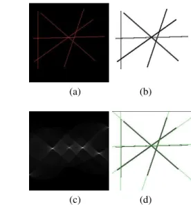
In order to validate the present proposal, the UCSB dataset [12] was employed. This dataset is composed by six reference images, shown in Figure 4, and 96 videos, with a total of 6889 frames. The videos are divided into groups according to the presented images transformations. In this work only the ”unconstrained” sequence was used, because it presents several kinds of images transformations, such as scale, rotation and changes in lighting.
The first experiment realized was the execution of the BRISK algorithm over the reference images. It was useful to conclude that, among the six images, two of them were not proper to be used as reference images with BRISK as the local features extractor. Namely, ”sunset” and ”wood”, do not present enough corners to be detected as keypoints by the extractor. The Table I presents the number of keypoints de-tected in each reference image. For the chosen video sequence
Fig. 4. Texture Images - (a) bricks (b) building (c) mission (d) paris (e) sunset (f) wood.
Fig. 5. Frames per second (FPS) average and standard deviation (in parenthesis), and hit rate, obtained for each video sequence concerning all three MAR frameworks.
all the MAR frameworks mentioned in the Section III were evaluated. As evaluation metrics were used the average frames per second (FPS) and the standard deviation, as well as, the hit rate, which is the percentage of frames where the reference objects were successfully detected. It can be observed that the Switching approach presents the better FPS averages for all sequences, as well as, the larger standard deviations. It can be explained by the greater number of times that there is a change between the detection and the tracking routines. Also considering the hit rate metric, theSwitchingframework presented more interesting results.
In Figure 6 some problems related with the pose of the de-tected object are shown. It happens before the pose restrictions imposition. Figure 7 shows the final result of a correct object pose (bounding box), limiting the internal angles. In this figure one can note the problem in the second picture, under the De-tection and Trackingapproach. It happened because keypoints positions became corrupted along the KL tracking process. The third image shows theSwitching approach where object is tracked correctly in a challenging pose. Finally, Figure 8 shows two sample frames with a 3D object augmentation over two different reference images.