Essays on economics of marriage

(1)

FUNDAÇÃO GETULIO VARGAS ESCOLA DE ECONOMIA DE SÃO PAULO

LORENA HAKAK MARÇAL

ESSAYS ON ECONOMICS OF MARRIAGE

(2)

FUNDAÇÃO GETULIO VARGAS ESCOLA DE ECONOMIA DE SÃO PAULO

ESSAYS ON ECONOMICS OF MARRIAGE

Tese apresentada ao Programa de Pós-Graduação da Escola de Economia de São Paulo da Fundação Getulio Vargas, como requisito à obtenção do título de Doutor em Economia de Empresas.

Orientador: Daniel Monte

(3)

Marçal, Lorena Hakak.

Essays on economics of marriage / Lorena Hakak Marçal. - 2016. 77 f.

Orientador: Daniel Monte

Tese (doutorado) - Escola de Economia de São Paulo.

1. Teoria dos casamentos. 2. Educação. 3. Renda - Distribuição. 4. Teoria dos jogos. I. Monte, Daniel. II. Tese (doutorado) - Escola de Economia de São Paulo. III. Título.

(4)

ESSAYS ON ECONOMICS OF MARRIAGE

Tese apresentada à Escola de Economia de São Paulo da Fundação Getulio Vargas, como requisito para obtenção do título de Doutor em Economia de Empresas. Data de aprovação: 20/06/2016.

Banca Examinadora:

Prof. Dr. Daniel Monte

(Escola de Economia de São Paulo)

Prof. Dr. Sergio Pinheiro Firpo (INSPER)

Prof. Dr. Luís Fernando Oliveira de Araújo (Escola de Economia de São Paulo)

Prof. Dr. David Daniel Turchick Rubin (FEA-USP)

(5)

(6)

AGRADECIMENTOS

(7)

ABSTRACT

Society has changed in the past decades raising questions to be asked by social scientists and their impacts on family units. In this thesis we aim to analyze how agents’ decisions on marriage and education can be interconnected assuming that men and women have preferences for intra-group marriage. In our framework we find that preferences for intra-group marriage can increase the proportion of men and women who decide to get married and study. We also show that empirically for Brazilian data there is a positive assortative mating between people with same traits, such as, education, religion or race. In addition, married couples that share the same religion tend to have the same level of schooling. We investigate how changes in marital sorting, educational composition and returns to education that occurred in Brazil in the last years can impact in household income inequality. We calculate counterfactual scenarios for Gini Coefficient keeping one of these three variables fixed in one year and comparing the counterfactual values with the actual one. If marriage were formed randomly, the Gini Coefficient would be lower than the actual one. Keeping the returns to education fixed in year 2014 we also show that the counterfactual Gini would be lower than the actual one.

Keywords: Matching, marriage market, assortative mating, education, family economics, cultural traits, household income inequality.

(8)

RESUMO

A sociedade mudou nas últimas décadas abrindo a possibilidade para cientistas sociais estudarem essas mudanças e analisar os seus impactos na unidade familiar. Nesta tese pretendemos analisar como as decisões dos agentes com relação a decisão de casar e estudar pode estar conectado considerando que homens e mulheres têm preferências pelo casamento intragrupo. No modelo estudado encontramos que as preferências para o casamento intragrupo podem aumentar a proporção de homens e mulheres que decidem se casar e estudar. Mostramos também que empiricamente há um positive assortative mating entre pessoas com as mesmas características, tais como, educação, religião ou raça. Além disso, a probabilidade de casais casados na mesma religião aumenta a probabilidade dos casais estarem casados dentro do mesmo nível de escolaridade. Considerando as mudanças em como os casais se formam, a composição educacional e os retornos da educação que aconteceram no Brasil nos últimos anos, investiga-se os impactos dessas mudanças na desigualdade de renda dos casais. Calculamos cenários contrafactuais para o Coeficiente de Gini mantendo uma dessas três variáveis fixas em um determinado ano, comparando o contrafactual estimado com o Gini real. Se o casamento for formado aleatoriamente com relação à educação, o Coeficiente de Gini seria menor do que o real. Mantendo os retornos da educação fixos no ano de 2014 encontramos um Gini contrafactual menor do que o real.

Palavras-chave: Matching, Mercado de casamento, assortative mating, educação, economia da família, características culturais, desigualdade de renda da família.

(9)

List of Figures

1.1 Regions for Marriage and Investment in Schooling . . . 9 2.1 Proportion of couples that both spouses have College Degree (PNAD) . . . 33 2.2 Proportion of uneducated men and women (PNAD) . . . 34 2.3 Proportion of men and women with College graduate (PNAD) . . . 34 2.4 Proportion of Educational Attainment of wives and husbands (PNAD) . . 35 2.5 Brazil and household income inequality: Changes in Marital Sorting . . . . 39 2.6 Brazil and household income inequality: Changes in Marital Sorting . . . . 40 2.7 Brazil and household income inequality: Changes in Educational

(12)

List of Tables

2.1 Couples formed with the same Level of Schooling, 1992 and 2014 (PNAD) 33

2.2 Summary Statistics, 1992 and 2014 (PNAD) . . . 35

2.3 Impacts of Levels of Education on Log-wages, 1992 and 2014 (PNAD) . . . 36

2.4 Marital Sorting Parameters, 1992 and 2014 (PNAD) . . . 37

2.5 Weighted average of Marital Sorting Parameters along the diagonal, 1992 and 2014 (PNAD) . . . 38

3.1 Couples formed with the same religion (Census 2000) . . . 47

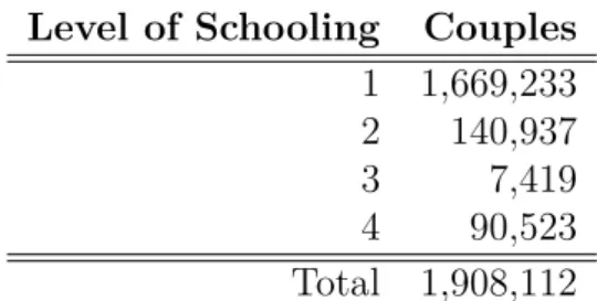
3.2 Couples formed with the same level of schooling (Census 2000) . . . 48

3.3 Couples formed within the same race (Census 2000) . . . 48

3.4 Total Men and Women in Religion Category (Census 2000) . . . 49

3.5 Percentage of Educated Men and Women (College Degree) in Religion Category (Census 2000) . . . 50

3.6 Marital Sorting Parameters in Levels of Schooling (Census 2000) . . . 50

3.7 Marital Sorting Parameters in Religion (Census 2000) . . . 51

3.8 Marital Sorting Parameters in Race (Census 2000) . . . 51

3.9 Double Marital Sorting Parameters in Race conditional to Education, 1992 and 2014 (PNAD) . . . 52

3.10 Weighted Average of Marital Sorting Parameters in Race conditional to Education, 1992 and 2014 (PNAD) . . . 52

3.11 IV Probit Results (2000) . . . 55

3.12 Double Marital Sorting Parameters in Religion conditional to Education -Level 1 (Census 2000) . . . 56

3.13 Double Marital Sorting Parameters in Religion conditional to Education -Level 4 (Census 2000) . . . 56

3.14 Double Marital Sorting Parameters in Education conditional to Religion -Catholics (Census 2000) . . . 57

3.15 Double Marital Sorting Parameters in Education conditional to Religion -Jewish (Census 2000) . . . 57

(13)

3.17 Double Marital Sorting Parameters in Education conditional to Religion -African Brazilian (Census 2000) . . . 57 3.18 Double Marital Sorting Parameters in Education conditional to Religion

-Buddhism (Census 2000) . . . 58 3.19 Double Marital Sorting Parameters in Education conditional to Race

-Black (Census 2000) . . . 58 3.20 Double Marital Sorting Parameters in Education conditional to Race

-White (Census 2000) . . . 58 3.21 Double Marital Sorting Parameters in Education conditional to Race

-Asian (Census 2000) . . . 58 3.22 Double Marital Sorting Parameters in Education conditional to Race

-Pardo (Census 2000) . . . 59 3.23 Marital Sorting Parameters in Education between Jewish and Catholics

(Census 2000) . . . 59 3.24 Marital Sorting Parameters in Levels of Schooling between Protestants and

Catholics (Census 2000) . . . 59 3.25 Marital Sorting Parameters in Education between Black and White (Census

2000) . . . 59 3.26 Marital Sorting Parameters in Levels of Schooling between Asian and White

(14)

Chapter 1 Investment in Education and the

Marriage Market with Intra-group

Preference

Abstract

This paper models how agents’ marriage decisions and investment in schooling are related to ethnic intra-group preferences. The incentives of men and women to acquire education and get married can change depending on the preferences to marry with their own type. It is shown that under symmetric preferences over education, we have a unique equilibrium where agents have only incentives to marry within their groups. The proportion of agents who marry and study is larger than in Chiappori et al. (2009)´s framework due to the preference for marriage within his (her) own type. In equilibrium, men know they will get married with somebody of their own type and, by symmetry, there is a woman who share the same preferences. As marriage becomes more interesting with the preference for marriage within the group, education brings an extra surplus. Therefore, their best decision is to acquire education because they increase their marital surplus.

JEL classification: I21, J12, Z1,D13.

KEYWORDS: matching, marriage market, education, family economics, cultural traits.

Acknowledgements

(15)

1.1 Introduction

The pattern of educational attainment has been changing in the last decades in many countries around the world. Women are acquiring more education than men on average. This reality contrasts with the pattern observed years ago. Men used to have a higher level of education than women. It used to be more common to observe marriages between educated and uneducated spouses. An anecdotal example is that male doctors used to marry more frequently with nurses whereas nowadays they marry more often with female doctors.1

The discussion along the role of men and women in households is connected with changes we observe in the last decades. As a consequence of these changes we can consider that the division of labor intrafamily and in the labor market is diﬀerent in most Western societies. Until decades ago, women have devoted most of her time in childbearing and household work whereas men devoted his time in labor market. Comparative advantages that men and women have in their roles lead them to specialization and the search of being eﬃcient in their duties.

Since women have achieved higher levels of education and they are inserted in the labor market, the division of labor intrafamily between husbands and wives has altered. Women are sharing childbearing and household work with men. Perfects substitutes migrated to complementarity, wives are becoming less specialized in household work whereas husbands are spending more time in household work and both are inserted in the job market. Those changes can have a consequence over homogamy marriage in education.2

The decrease in the gender educational gap raises the probability that an educated woman marries an educated man, even if the assortative pattern has not been changed. Considering the existence of complementarity between couples’ traits in the production of utility, which is illustrated by a higher marital surplus, the incidence of homogamous marriage tends to increase even more. This tendency probably aﬀects income distribution as well.3 _{Freeman (1955),Finkel et al. (2012),Bisin and Verdier (2000)}

The preference for homogamous marriage between spouses can be related not only to education but with other traits such as religion and ethnicity. There is a large literature that discusses the importance for a couple to transmit their traits to their children. One of the strongest mechanisms to achieve this goal is throughout marriage.4

In this paper, we intend to discuss how preferences for marriage with spouses of similar traits can aﬀect investment in education and marriage. Moreover, in some situations, those that prefer to homogamous marriage can decide to invest in education in order

1_{Article "Sex, brains and inequality" published in 02/08/2014 by The Economist.} 2_{Chiappori et al. (2009) and Becker (1991).}

3_{Homogamous marriage can be defined as a marriage between people who are similar in cultural traits,}

educational level, religion, ethnicity, socioeconomic status, among others.

(16)

to get married. This can happen because the greater the return to marriage between people of the same type, the greater are the incentives to study and marry. All in all, we are interested in analyzing the relationship between agents with diﬀerent traits and its implication for education and marriage.

Under symmetric preferences we are able to show that agents will marry within his (her) own type and assortative in Education. We show that there is a unique equilibrium with homogamous marriage. Our model is based on Chiappori et al. (2009)’s work.

Chiappori et al. (2009) developed a model where the investment in education generates two different types of returns. The first one is in the labor-market and the second is in the marriage market. Moreover, both men and women can have different incentives to acquire education because they can have different household roles, which leads to different market wage.

They showed that a unique equilibrium exists even though it could be a "symmetric" equilibrium or mixed one.5 _{It depends on whether there is gender equality in the labor}

market and it will be reﬂected in the share of utility that each spouse earns from the marriage.

Furthermore, there is a debate on how family values are transmitted throughout generations. Parents might not be indifferent to their children’s preferences to religious, ethnic and cultural traits. Marriage can be an important mechanism to transmit those traits through family socialization and homogamous marriage. According to Bisin and Verdier (2000), social scientists in the first half of the 20th century used to agree that American society would become more homogeneous, that is, a melting pot hypothesis. The assimilation of immigrants would transform the American society, from their differences in ethnic, into a common culture whereas the evidence nowadays does not support this view anymore.

New York is an emblematic city that reflects the failure of a melting pot theory. The city is divided into different ethnic groups, such as, Italian, African Americans, Jews, Chinese, Latin, etc. Glazer (2000), Glazer and Moynihan (1963) suggest that the assimilation between different ethnic groups in New York has grown a little but it is far from ensure it is becoming a melting pot. In addition, we can share other examples outside the United States. Jews and Muslims around the world have remained attached to their cultural traits through the centuries. The Basques and Catalans in Spain too. Borjas (1994) presents a work which suggests that the performance of workers can be related not only to parental skills but also the nature of an ethnic externality and how it might operate. The paper shows that in the United States there is a strong evidence of residential segregation and ethnic externalities.

Lehrer (2004) examined the role of religiosity as a determinant of educational 5_{The returns of education are symmetric between men and women. And there is a positive assortative}

(17)

attainment within speciﬁc genders and faiths. The empirical analysis showed that women raised as conservative Protestants who attended religious services more than once a week when they were teenagers achieved one more year of schooling. She compared a more religious group of Protestants women with a less religious one. According to Sander (2010), the family religious background (Islam and Judaism) can interfere on educational attainment in United States agents. And the decision of acquiring more years of schooling has an important impact on income and economic mobility.

If this intergenerational transmission is considered an important legacy probably there will be search for marriage within the group type. In addition, a minority group can have more incentives to search for a homogamous marriage than a majority group because in a heterogamous marriage the minority type will have more diﬃculties to transmit their traits. The role models and peers will prevail from the majority group.6 _Moreover,

Lehrer and Chiswick (1993), Waite and Lehrer (2003) and Becker (1991) showed that it is reasonable to assume that homogamous marriage tends to be more stable than mixed marriage, thus turning the homogamous marriage more attractive.

The marriage decision can inﬂuence the decision on education and the level of schooling can aﬀect earning capacity and job opportunities in the labor market. Our model aims to analyze the possible interaction in homogamous marriage between men and women of the same type and education. We show that under symmetric preferences agents will marry within their own type and with the same level of schooling. There will be no incentives to marry outside their own type. We show there is a unique equilibrium with homogamous marriage both in type and education.

This paper is organized as follows. In the next section, we examine the related literature. The third section we develop our model and in the fourth we present the equilibrium. In the ﬁfth section we present some limitations and possible extensions of our model. Finally, in Section 6 we present some ﬁnal remarks.

1.2 The Model

Shapley and Shubik (1971) have solved the assignment game as a linear programming problem. We present a two-sided matching model with transferable utility and complete information based on Chiappori et al. (2009), where agents intend to maximize the aggregate marital surplus over all possible assignments considering they share diﬀerent traits.

(18)

1.2.1 Definitions

In the ﬁrst part we will present an overview of Chiappori et al. (2009)’s framework. The model is based on the assumption that there are two equally large populations of men and women to be matched. Agents live for two periods. In the ﬁrst period the agent chooses to acquire education or not, and in the second, if he (she) will get married and with whom. Wages are assumed to be exogenous.

There are two ﬁnite and disjoint sets of men and women, each of them represented by letters P and Q. Each set containsp and q players, respectively. The letters i and j will indicate agents of each set and a partnership of (i, j) inP×Qwill generate a nonnegative marital surplus sij.7

The utility provided from marriage can be divided in two parts. The ﬁrst one is deﬁned as a material surplus and the second one is an emotional gain. Material surplus is generated by a material output (ξI(i)J(j)) formed by the union between husbandi and

wifej discounted by the output that each spouse produce when single, whereI(i)and J(j)

represents the level of education of each spouse. This material surplus depends on the level of education of both spouses which can be uneducated or educated, represented by 1 and 2 respectively.

Men and women choose whether they will study or not. If he (she) decides to study in the ﬁrst period, he (she) works only in the second one and he (she) earns ξ20. If he

(she) chooses not to study, he (she) works in both periods and he (she) earns 2ξ10. The

absolute return of education for men and women who never get married is represented by

RP ₌_ξ

20−2 ξ10 and RQ=ξ02−2 ξ01.

The material surplus is:

ZI(i)J(j)=ξI(i)J(j)−ξI(i)0−ξ0J(j) (1.1)

Emotional gains are idiosyncratic variables generated by preference for marriage represented by θi and θj. Investment in education is associated to idiosyncratic costs µi

orµj. Agents search for partners in order to maximize their share in wedding surplus. It

is assumed that the educational levels are complementary between agents in the marriage as in Becker (1973)’s deﬁnition of positive assortative mating, that is,

Z11+Z22 > Z12+Z21 (1.2)

The matching outputZ(I(i), J(j)) is supermodular inI(i) andJ(j) and it is considered that

Z12 =Z21 (1.3)

(19)

from typesγ ∈ {A, B}.The number of men and women within group is the same but can diﬀer between groups. We add an idiosyncratic parameter, the type gains, represented byλi and λj. These parameters are generated by intra-group marriage. We assume that

the idiosyncratic parameters θi , µi, and λi are independent from each other and across

all individuals. We denote G(µ) as the distribution of µ, and F(θ) as the distribution of θ, symmetric around its zero mean. We denote by H(λ) the distribution of λ which is continuous and deﬁned on a positive interval. The probability distribution function (p.d.f.) h(λ) will be zero outside this interval. The p.d.f. f(θ) is a distribution where the probability of the values decrease monotonically as they become more distance from the mean.

We consider in our model that men and women are completely symmetric in their preferences as deﬁned as follow. Consider a type proﬁle tγi = (λi, θi, µi). Men, reported

byi, have a type proﬁle tγi ∈Πγp which is the type space and women, reported by j, have

a type proﬁletγj ∈Πγq (type space). We assume that:

ΠA

p = Π

A

q (1.4)

ΠB

p = ΠBq (1.5)

The joint distribution of the three characteristics λ, θ, µ is described as a function Σ such that for all values of µ, θ, λ (Σ :R×R×R+ _→₍₀_,₁₎₎_,

The function is given by Σγ_p₍_q₎(λ, θ, µ) =H(λ).F(θ).G(µ) and we assume that:

ΣA

p(t) = ΣAq(t) (1.6)

ΣB

p(t) = Σ B

q(t) (1.7)

The marital surplus (Sij) depends on the educational levels of the partners and their

types (A orB).

sij =

 



ZI(i)J(j)+θi+θj if γi 6=γj

ZI(i)J(j)+θi+θj +λi+λj if γi =γj

(1.8) The surplussij will be distributed between the players and, under transferable utilities,

woman j receivesuj and man i receivesvi.

1.2.2 Stability and Equilibrium Conditions

(20)

uj ≥0, vi ≥0 (1.9)

and

uj +vi ≥sij∀(i, j) in P ×Q. (1.10)

Stability requires that the conditions (1.9) and (1.10) be satisfied. Otherwise the outcome followed from the maximization problem is not feasible. In condition (1.9) is defined that men and women can always remain single if they want, so their payoff would beuj = 0,vi = 0.The condition (1.10) presents the notion that if a maniand a woman j

decides to marry they will not have an incentive to deviate from this partnership. There will be no other partnership that formed with one of them that will lead to a higher payoﬀ and block the original partnership.

Agents maximize their marital surplus considering that their peers are doing the same. The problem of linear programming developed by Shapley and Shubik (1971) shows that any stable matching between men and women emerges from the problem of maximization of the aggregate surplus among all possible assignments.

vi = max

 



maxj

nh

ZI(i)J(j)+θi+θj−uj

i

,0o if γi 6=γj

maxj

nh

ZI(i)J(j)+θi +θj +λi+λj−uj

i

,0o if γi =γj

(1.11)

uj = max

 



maxi

nh

ZI(i)J(j)+θi+θj −vi

i

,0o if γi 6=γj

maxi

nh

ZI(i)J(j)+θi+θj+λi+λj−vi

i

,0o if γi =γj

(1.12)

The shares uj and vi are determined endogenously and we can write them as:

vi = max (VI+θi+λi,0) (1.13)

and

uj = max (UJ+θj +λj,0) (1.14)

whereVI and UJ represent the material surplus husbands and wives earn from marriage.

When agents search for their partners they already know VI and UJ.

VI = max

(21)

and

UJ = max

I [ZIJ −Vi] (1.16)

Education and Investment Decision

Men and women need to decide whether or not they will invest in education. Considering rational expectations, that is, in equilibrium husbands and wives know the shares they receive from material surplus. Their choice to invest in education depends on the shares provided from material surplus and the values of their idiosyncratic parameters

θ, λ and µ. After that, they will be sure if they will get married or remain single in the second period conditional to their choice of be educated or not. According to conditions (1.19) to (1.24), men will be divided among the areas in Figure 1. Some of them will not get married and not study, others will not get married but invest in education or get married but not invest in education and part of them will marry and invest.8

Mani of type A(B) will invest in education if:

ξ20−µi+ max (V2+θi+λi,0)>2ξ10+ max (V1+θi +λi,0), (1.17)

Womanj of type A(B) will choose to invest in education if:

ξ02−µj+ max (U2+θj+λj,0)>2ξ01+ max (U1+θj+λj,0), (1.18)

Conditions and thresholds are described below: Mani with

θi <−(V2+λi) (1.19)

will not marry. And he will invest in education if

µ < ξ20−2ξ10=RP (1.20)

Man i with

θi >−(V1+λi) (1.21)

will marry and will decide to invest in education or not if and only if

µ < RP +V2−V1 (1.22)

In this situation, man will always get married but he will decide to study if the return from education (RP_{) adding the returns to schooling in marriage, which depends on his}

decision to study or not (V2−V1), will be greater than his idiosyncratic cost of schooling

µ.

8_{See appendix C for a numerical example. We present the thresholds in a similar way as in Chiappori,}

(22)

Finally, if

−(V2+λi)< θi <−(V1 +λi) (1.23)

than man will marry only if he acquires education and the condition will be

µ < RP +V2+θi+λi (1.24)

The return from education adding the material share from marriage and the idiosyncratic emotional gain θ and the type gain λ must be greater than µ, otherwise man will not marry. These conditions hold for women too.

Figure 1.1: Regions for Marriage and Investment in Schooling

Which type men and women are going to marry with?

Agents need to decide whether or not they will get married within his (her) own type. Consider a market with men and women which satisﬁes the following two assumptions: 1. They have symmetric preferences (conditions (1.4) and (1.5)) and symmetry in

gender (condition (1.3)) and

RP =RQ (1.25)

2. The condition (1.2) holds.

Consider that, in equilibrium, men and women know their material surplus and it is characterized by equal sharing, that is, V2 = U2 = Z22/2 and U1 = V1 = Z11/2.

(See appendix A)

(23)

Proof. Suppose man 1 has his type preferences θ1, λ1 and µ1. According to conditions

((1.19) to (1.24)) he will decide to invest in schooling or not. Consider θ1 >−(V1+λ1)

and suppose man 1 has µ1 < RP +V2 −V1. In this case he will decide to study. By

symmetry, there is a woman 2 with the same characteristics of man 1 (θ1, λ1 and µ1),

but she decides not to study. In this case her µ1 should be greater than RQ+U2 −U1.

According to conditions (1.21), (1.22) and symmetry in gender, µ1 < RQ+U2 −U1 , a

contradiction.

Proposition 2. (Preferences for intra-group marriage) If a man (or woman) wishes to marry then he (she) will marry with someone from his (her) own type.

Proof. Consider a market with men and women who share the same preferences over education and marriage according to conditions ((1.4) , (1.5), (1.2) and λi > 0). We

will show that couples formed by agents of the same type will result in equilibrium (in order to achieve equilibrium, conditions (1.13), (1.14), (1.15) and (1.16) must be satisﬁed). Suppose man A (B) solves his maximization problem and is assigned to woman B (A) and they receive from marital surplusVI(1)+θ1 and UJ(2)+θ2 respectively. There is a woman

A (B) who, from symmetry conditions ((1.4) and (1.5)), shares the same preferences of man A (B). Then by lemma 1, they have the same decision about schooling. Suppose she solves her maximization problem and is assigned to man B (A) and they receive from marital surplus VI(2) +θ2 and UJ(1) +θ1 respectively. But if man A(B) marries woman

A(B), together they will be better oﬀ. They will receive from marital surplusVI(1)+θ1+λ1

and UJ(1)+θ1+λ1. The same holds for man and woman B. So, marriage between mA

and wA and mB and wB blocks marriage between mA and wB and mB and wA.

The proportion of men who decide to marry or remain single and decide to invest in schooling or remain uneducated.

According to proposition 2, there will not be mixed marriage between types (γǫ{A, B}). So, in order to draw Figure 1, we can compute the proportion of men who marry, get educated, remain single or not invest in schooling by each type separately. The same holds for women.

The proportion of men of type A (B) who marry is:

Λ =

ˆ +∞

0

ˆ −₍V1+λi)

−₍V2+λi)

G(RP+V2+θi+λi)f(θ)h(λ)dθdλ+

ˆ +∞

0

{1−F[−(V1+λi)]}h(λ)dλ

(1.26) where G(Rp ₊_V

2 +θi +λi) =

´Rp+V2+θi+λi

−∞ g(µ)dµ and {1−F[−(V1+λi)]} = 1−

´−₍V1+λi)

−∞ f(θ)dθ. The left side of the equation represents the proportion of men who have

(24)

represents the proportion of men that have their preferencesθi >−(V1+λi) for any µor

λ.

Proportion of men of type A (B) who invest in schooling is:

Ψ =

ˆ +∞

0

G(RP₎_F_[₋₍_V

2+λi)]h(λ)dλ+ (1.27)

ˆ +∞

0

ˆ −₍_V₁₊_λ_i₎

−₍V2+λi)

G(RP ₊_V

2+θi +λi)f(θ)h(λ)dθdλ+

ˆ +∞

0

{1−F[−(V1+λi)]}G(RP +V2−V1)h(λ)dλ

The ﬁrst part of the equation shows the proportion of men who invest in schooling because their isµ < Rp _{but their preferences for marriage}_θ

i <−(V2+λi).The next part

of the equation represents the proportion of men who have their preferences for marriage (θ) between −(V2+λi) and −(V1+λi) and they invest in schooling because their cost

of education µ < Rp₊_V

2 +θi +λi. And the right side represents the proportion of men

who invest in schooling because their cost of schooling is µ < Rp ₊_V

2 −V1 and their

θi >−(V1 +λi) for any λ.

The proportion of men of type A (B) who invest and marry is:

Ω =

ˆ +∞

0

ˆ −(V1+λi)

−₍V2+λi)

G(RP+V2+θi+λi)f(θ)h(λ)dθdλ+ ˆ +∞

0

{1−F[−(V1+λi)]}G(RP+V2−V1)h(λ)dλ

(1.28)

where the left side of equation represents the proportion of men who have their preferences for marriage (θ) between−(V2+λi) and−(V1+λi) and they invest in schooling because

their cost of educationµ < RP ₊_V

2+θi+λi and the right side represents the proportion

of men who invest in schooling because their cost of schooling is µ < RP ₊_V

2 −V1 and

their θi >−(V1+λi) for any λ.

It is possible to divide men between those who decide to marry or remain single, and invest in schooling or not. Figure 1 brings the limits of integration and the thresholds (conditions (1.19 to 1.24) where we can see the proportion of those men who invest or not in schooling, get married or remain single. It is a three dimensional graph but in order to make easier to visualize the eﬀects on the change in the areas caused byλand compare to a similar picture from Chiappori et al. (2009), we represent the graph in a two-dimensional way (θ, µ) keeping λ ﬁxed. As λ increases, the boundaries of the marriage area shifts to the left.

(25)

where a parameter c multiplies λ. As we can check, when c = 0, we are in Chiappori et al. (2009)‘s environment. It holds for functions (1.26) and (1.28) as well.

Ψ′

=

ˆ +∞

0

G(RP)F[−(V2+cλi)]h(λ)dλ

+

ˆ +∞

0

ˆ −(V1+cλi)

−₍V2+cλi)

G(RP +V2+θi+cλi)f(θ)h(λ)dθdλ

+

ˆ +∞

0

{1−F[−(V1+cλi)]}G(RP +V2−V1)h(λ)dλ (1.29)

Λ′

=

ˆ +∞

0

ˆ −₍V1+λi)

−(V2+λi)

G(RP +V2+θi+cλi)f(θ)h(λ)dθdλ+ ˆ +∞

0

{1−F[−(V1+cλi)]}h(λ)dλ

(1.30)

Ω′

=

ˆ +∞

0

ˆ −₍V1+λi)

−₍V2+λi)

G(RP +V₂+θi+λi)f(θ)h(λ)dθdλ

+

ˆ +∞

0

{1−F[−(V1+λi)]}G(RP +V2−V1)h(λ)dλ (1.31)

Proposition 3. (The role of intra-group type parameter λ in education and marriage) Using the equations (1.29), (1.30) and (1.31), it is possible to show that: The change in the proportion of men who wish to study or marry is a positive function of parameter c, ∂Λ′

∂c >0. The same holds for women.

In the new context, there are three effects in the proportion of men who marry and study. According to Proposition 3, in the pink area, men who before were willing to study but not get married will change their decision and marry. In the green area, more men will decide to marry but they will not invest in schooling. As a effect of λ in these two regions men will decide to marry but will not change their decision to study, whereas, in the yellow area, the increase inλwill change their decision about schooling. In this region their decision to study will change because of the idiosyncratic type parameterλ and the preferences to marry within their own type. They will study in order to get married. The proportion of men who study and marry increases. The same holds for women. We can check these effects considering Proposition 3.

(26)

∂Λ′

∂c =

ˆ +∞

0

f[−(V1+cλi)]

h

1−G(RP ₊_V

2−V1)

i

λih(λ)dλ+

ˆ +∞

0

ˆ −₍V1+cλi)

−₍V2+cλi)

g(RP ₊_V

2+θi+cλi)λif(θ)h(λ)dθdλ

+

ˆ +∞

0

G(RP₎_f₍₋_V

2−cλi)λih(λ)dλ >0 (1.32)

The derivative is positive then as cincreases, the proportion of men who get married rises.

We evaluate the derivative at point c= 0.

∂Λ′

∂c (c= 0) =

ˆ +∞

0

f(−V1)λih(λ)dλ

h

1−G(RP ₊_V

2−V1)

i

+

ˆ +∞

0

ˆ −₍V1)

−₍V2)

g(RP +V2+θi)λif(θ)h(λ)dθdλ

+

ˆ +∞

0

G(RP₎_f₍₋_V

2)λih(λ)dλ >0 (1.33)

A marginal increase inchas an impact on the proportion of men who decide to marry, comparing with Chiappori et al. (2009)‘s environment where c= 0.

Case 2: Consider the function (1.31). We want to study the impacts on schooling and marriage caused by changes inc.

∂Ω′

∂c =

ˆ +∞

0

f[−(V1+cλi)]λiG(RP +V2−V1)h(λ)dλ+ (1.34) ˆ +∞

0

ˆ −(V1+cλi)

−₍_V₂₊_cλ_i₎

g(RP ₊_V

2 +θi+cλi)λif(θ)h(λ)dθdλ−

ˆ +∞

0

G(RP +V2−V1)f(−V1 −cλi)λih(λ)dλ+

ˆ +∞

0

G(RP)f(−V2−cλi)λih(λ)dλ >0

We evaluate the derivative at point c= 0.

∂Ω′

∂c (c= 0) =

ˆ +∞

0

ˆ −V1

−_V₂

g(RP ₊_V

2+θi)λif(θ)h(λ)dθdλ+ (1.35)

ˆ +∞

0

G(RP₎_f₍₋_V

(27)

Case 3: Consider the function (1.27). We want to study the impacts in schooling caused by changes inc.

∂Ψ′

∂c = +

ˆ +∞

0

f[−(V1+cλi)]λiG(RP +V2 −V1)h(λ)dλ+ (1.36) ˆ +∞

0

G(RP)f(−V2−cλi)λih(λ)dλ+

ˆ +∞

0

ˆ −(V1+cλi)

−(V2+cλi)

g(RP +V2 +θi+cλi)λif(θ)h(λ)dθdλ+ −

ˆ +∞

0

G(RP +V2−V1)f(−V1−cλi)λih(λ)dλ−

ˆ +∞

0

G(RP)f(−V2−cλi)λih(λ)dλ

=

ˆ +∞

0

ˆ −(V1+cλi)

−₍_V₂₊_cλ_i₎

g(RP +V2 +θi+cλi)λif(θ)h(λ)dθdλ >0

We can evaluate the derivative at point c= 0.

∂Ψ′

∂c (c= 0) =

ˆ +∞

0

ˆ −V1

−V2

g(RP ₊_V

2+θi)λif(θ)h(λ)dθdλ >0 (1.37)

The derivative of the area with respect to c is positive (1.32). An increase in c leads to a raise in the proportion of men who marry comparing to Chiappori et al. (2009)’s framework. This can be related directly to agents’ preferences over marriage within their own type.

The same result is achieved by the proportion of men who marry and acquire education (condition (1.28)) and the proportion of men who study (function (1.27)) as shown in equations (1.34) and (1.36). 9

The derivatives evaluated inc= 0 (equations 1.33 to 1.37) shows a comparative statics of our model in relation to Chiappori et al. (2009). It suggests that the introduction of a new idiosyncratic variable conditional to be part of a intra-group marriage can aﬀect decisions of studying and getting married.

One interesting question that arises from our paper is how agents decisions about education and marriage are affected by changes inλ. As we can see from proposition (3), changes in cλ can affect their decisions of schooling and marriage. There are two kinds of men. Part of them who wants to marry anyway, that is, they want to marry within their group or not. Their preference for marriage is high but they will end up married with someone from their own group because of the parameterλ. And part of them share a low preference for marriage. But as an effect of preference for marriage with someone of his own trait, they can marry. In equilibrium, they know they will get married with somebody of their own type and, by symmetry, there are some women who share the same

(28)

preferences. So, they decide to marry. And in order to achieve marriage, they can decide to acquire education. This result suggests that people can acquire education in order to marry his own type because they can increase their material surplus through education. The same result holds for women.

1.3 Equilibrium

In equilibrium, the proportion of husbands and wives of type A (B) who get married need to be equal.10 _{From equation (1.26) and applying symmetry of}_F ₍_θ_{), we present the}

following condition

ˆ +∞

0

ˆ (V2+λi)

(V1+λi)

G(RP +V2−θi+λi)f(θ)h(λ)dθdλ

+

ˆ +∞

0

F (V1+λi)h(λ)dλ

=

ˆ +∞

0

ˆ (U2+λj)

(U1+λj)

G(RQ+U2−θj +λj)f(θ)h(λ)dθdλ

+

ˆ +∞

0

F (U1+λj)h(λ)dλ (1.38)

where the left-hand of (1.38) represents the proportion of husbands and the right-hand side denotes the wives’ side.

There will be only homogamous marriage, that is, educated men and women marry with each other and the same holds for uneducated men and women. From proposition 2, men of type A (type B) marry only women of type A (type B). Then, we can divide the group of men and women in four disjoint groups: men of type A (type B) and women of type A (type B). We split our problem in two subgroups: men and women of type A and men and women of type B. And we can show that in each market the equilibrium exists and is unique. In this situation, we have two markets composed by men and women of type A and men and women of type B.

Having positive assortative mating, we consider condition (1.26) so the proportion of educated (uneducated) men who marry must be the same of the proportion of educated (uneducated) women who marry. Using condition (1.28) and symmetry ofF (θ), we have the following condition:

H(0){F(V1+λi)[1−G(RP+V2−V1)]}=H(0){F(U1+λj)[1−G(RQ+U2−U1)]} (1.39)

(29)

where H(0) = ´+∞

0 h(λ)dλ. The left side of the equation represents the proportion

of uneducated men that get married. This area is represented in Figure 1.1 in the regions green and blue. The right side of the equation represents the proportion of uneducated women who get married.

In this condition we consider that we have an equal number of uneducated men and women who get married. The equilibrium, in this case, satisﬁes (1.39), (1.38),

U1+V1 =Z11

and

U2+V2 =Z22

. We show in Appendix B that there is a unique equilibrium with homogamous marriage in each group A and B.

1.4 Limitations and Possible Extensions

The present work analyzed marriage decision between people that belong to different groups and they have preference for intra-group marriage. In this framework, under symmetric preferences, we can show that there is a unique equilibrium with homogamous marriage. It will be very interesting to develop a model that could explain the mixed marriage between people from different types. What kind of asymmetry can induce mixed marriage? In addition, we can ask why there is an increasing trend in mixed marriage nowadays related with some minority groups than there was decades ago? Kalmijn (1998) One possible explanation can be related to a searching problem. Petrongolo and Pissarides (2001) In some countries, these minority groups no longer live in the same neighborhood or are isolated from the rest of society and that could explain why it is hard to find a match from the same type. 11

The mechanism to transmit ethnic traits through marriage is still strong within some groups. Nevertheless, women household role changed in some countries and both men and women in those societies are feeling more free to search for their partners. Moreover, as social norms have changed, women are investing more in schooling and spending less time working at home.12

The changes in segregated neighborhoods, social norms and women household role can make more difficult for men (women) to find a match within their own type. In such both cases, if men and women intend to marry within their own type, best strategy should be improve educational level in order to increase his payoff and become more attractive to a potential partner. This could be a reason why some minorities have higher educational 11_{Bisin et al. (2004)}

(30)

attainment than majority groups.13 _{And in the case they do not ﬁnd someone from}

own type, with a higher educational level, they can be more competitive in the market and marry with an educated person. In both situations, they will earn a higher marital surplus.

1.5 Conclusion

In this work we model how agents’ marriage and education decisions are related to ethnic intra-group preferences. Under symmetric preferences we are able to show that agents will marry within his (her) own type and assortative in Education. We show that there is a unique equilibrium with homogamous marriage.

Part of the agents wants to get married because their preference for marriage is high. So they want to get married anyway but they will end up married with someone from their own group because there is always a partner of his (her) own type (due to symmetry) that will accept to marry to gain the extra bonus from marrying someone of her (his) own type. So, they decide to marry. And, as they know they will get married, the channel to increase the return of marriage is to acquire education. This result suggests that people can acquire education in order to marry his own type. Men and women can increase their material surplus through education.

Comparing our model with Chiappori et al. (2009)’s framework we are able to show that agents will acquire education in order to improve their material surplus on the marriage. In this situation, he (she) wants to marry with someone of speciﬁc trait and he (she) knows, by symmetry, that there is a woman who will decide to study as well. So, the proportion of educated men and women are greater in our framework than in Chiappori et al. (2009).

We also show that there is no incentive to marry with mixed types. We left for future research to analyze the role of asymmetric returns in education over marriage market equilibrium in this framework.

1.A

Appendix A

In our framework the material sharesUJ and VI do not depend on type A or B.14And

it is possible to show this result.15

Consider men and women have symmetric preferences (1.4 and 1.5), symmetry in

13_{Sander (2010)}

(31)

gender (1.3 and 1.25) and condition (1.2) holds.16

The proportion of men who marry is:

2    ´+∞ 0

´−₍V1+λi) −₍V2+λi) G(R

P ₊_V

2+θi+λi)f(θ)h(λ)dθdλ

+´+∞

0 {1−F[−(V1+λi)]}h(λ)dλ

 



(1.42) The proportion of men who marry and study:

2    ´+∞ 0

´−₍_V₁₊_λ_i₎ −₍V2+λi) G(R

P ₊_V

2+θi+λi)f(θ)h(λ)dθdλ

+´+∞

0 {1−F[−(V1+λi)]}G(R

P ₊_V

2−V1)h(λ)dλ

 



(1.43) In the marriage market equilibrium, the proportion of men and women who marry have to be the same. Using equation (1.42) we can write the following condition:

ˆ +∞

0

ˆ −₍V1+λi)

−₍V2+λi)

G(RP₊_V

2+θi+λi)f(θ)h(λ)dθdλ+

ˆ +∞

0

{1−F[−(V1+λi)]}h(λ)dλ=

ˆ +∞

0

ˆ −₍U1+λi)

−(U2+λi)

G(RQ+U2+θi+λi)f(θ)h(λ)dθdλ+

ˆ +∞

0

{1−F[−(U1+λi)]}h(λ)dλ

(1.44) Considering strictly positive assortative mating, the proportion of men and women who are educated (uneducated) must be the same. In addition, we impose condition (1.44) and the number of men and women who marry and not study are the same. Using condition (1.43) and symmetry, we can derive this condition as

ˆ +∞

0

F[(V1+λi)]}

h

1−G(RP +V2−V1)

i

h(λ)dλ= (1.45)

ˆ +∞

0

F[(U1+λi)]}

h

1−G(RQ+U2−U1)

i

h(λ)dλ (1.46) Considering conditions

U1+V1 =Z11

and

U2+V2 =Z22

, (1.44) and (1.45), they provide a system with four equations and four unknowns.

16_{Consider also:}

ΠAp = ΠBp (1.40)

(32)

Consider the four conditions (1.44), (1.45),

U1+V1 =Z11

and

U2+V2 =Z22

. As the model is completely symmetric, it holds condition (1.3) and (1.25). We have from (1.3)U1+V2 =U2 +V1.Then,

U1−U2 =V1 −V2 (1.47)

Substituting (1.25) and (1.47) in (1.45), we have:

2 (

+

ˆ +∞

0

F[(V1+λi)]}

h

1−G(RP ₊_V

2−V1)

i

h(λ)dλ

)

= (1.48)

2 (

+

ˆ +∞

0

F[(U1+λi)]}

h

1−G(RQ₊_V

2−V1)

i

h(λ)dλ

)

To keep equality ⇒

V1 =U1 (1.49)

Substituting (1.49) in

V1 +U1 =Z11

we have the following result:

V1 =U1 =Z11/2 (1.50)

Substituting (1.49) in (1.47) we have

V2 =U2 (1.51)

So,

V22 =U22 =Z22/2 (1.52)

1.B

Appendix B

A) We intend to show existence and unicity of equilibrium:

(33)

Step 1:

Consider equation (1.28) and substitute for U2 = z22−V2 and U1 = z11−V1. Now

deﬁne a function Φ(V1, V2) as

Φ(V1, V2) =

ˆ +∞

0

ˆ (V2+λi)

(V1+λi)

G(RP ₊_V

2−θi+λi)f(θ)h(λ)dθdλ (1.53)

+

ˆ +∞

0

F(V1+λi)h(λ)dλ −

ˆ +∞

0

ˆ (U2+λj)

(U1+λj)

G(RQ₊_U

2−θj +λj)f(θ)h(λ)dθdλ −

ˆ +∞

0

F (U1+λj)h(λ)dλ

where H(0) =´+∞

0 h(λ)dλ

Φ(V1, V2) = H(0)

 



´(V2+λi)

(V1+λi) G(R P ₊_V

2−θi+λi)f(θ)dθ+F (V1+λi) −´(U2+λj)

(U1+λj) G(R Q₊_U

2−θj +λj)f(θ)dθ−F(U1+λj)

 



(1.54)

Φ(0,0) =H(0) (

F(λi)−

ˆ (U2+λj)

(U1+λj)

G(RQ+z22−θj +λj)f(θ)dθ−F(z11+λj)

)

<0 (1.55) and

Consideringz11>0 implies thatF (z11+λi)−F (λj)>0.By continuity, it is possible

to consider that there is a set of pairs (V1, V2) for which Φ(V1, V2) = 0.

Using the Implicit Function Theorem,

∂Φ(V1, V2)

∂V1

=H(b)  



f(V1+λi)−f(z11−V1+λj)−G(RP +V2−V1+λi)f(V1+λi) −G(RQ₊_z

22−V2−V1+λj)f(θ)dθ−F (z11−V1 +λj)

 

 = (1.56) H(b)nf(V₁+λi)

h

1−G(RP +V₂−V₁+λi)

i

−f(z₁₁−V₁+λj)

h

1−G(RQ+z₂₂−V₂+V₁+λj)

io >0

∂Φ(V1, V2) ∂V2

=H(0)

( ´(V₂+λi) (V1+λi) g(R

P₊_V

2−θi+λi)f(θ)dθ+G(RP)f(V1+λi)f(V2+λi)

+´(z22−V2+λj) (z11−V1+λj) g(R

Q₊_z

22−V2−θj+λj)f(θ)dθ(−1) +G(RQ)f(z22−V2+λi) )

>0

(1.57)

According to the Implicit Function Theorem, the derivative ∂V2

∂V1 is negative so the

function Φ(V1, V2) is a decreasing curve in the (V1, V2) plane.

(34)

Using (26), deﬁne Θ(V1, V2) as

Θ(V1, V2) =H(0)F(V1+λi)1−G(RP+V2−V1)−F(z11−V1+λj)1−G(RQ+z22−V2−z11+V1)

(1.58)

Note that Θ is continuously diﬀerentiable, the derivative of Θ(V1, V2) with respect of

V1 is increasing and decreasing with respect toV2. In addition:

limV1→∞Θ(V₁, V₂) = H(0){1−0} −H(0){0}=H(b)

limV2→∞Θ(V₁, V₂) = H(0){[F (V₁+λ_i) 0]−[F (z₁₁−V₁ +λ_j) (1−0)]} = −H(0)F (z11−V1+λj)<0

There is a locus that satisﬁes Θ(V1, V2) = 0, considering continuity. From the implicit

function theorem, it is possible to obtain an increasing curve in the (V1, V2) plane.

Moreover, Θ(V1, V2) =A(V1, V2−V1) whereV1 =V and V2−V1 =X, where

A(V, X) =H(0)

F(V +λi)

1−G(RP +X)

−F(z11−V +λj)

1−G(RQ+z22−X−z11)

Since ∂A(V, X)

∂V =H(0) n

f(V +λi)

h

1−G(RP +X)i+f(z₁₁−V +λj)

h

1−G(RQ+z₂₂−X−z₁₁)io>0,

∂A(V, X)

∂X =H(0) n

−F(V1+λi)g(RP +X)−F(z11−V +λj)g(RQ+z22−X−z11)

o <0,

from equation A(V, X) = 0 it is possible to deﬁneX as an increasing function φ of V. Therefore,

Θ(V1, V2) =A(V1, V2−V1) = 0

gives

V2−V1 =φV1

V2 =V1+φV1

(whereφ′₍

V)>0)

∂A(V, X)

∂V1

= ∂A(V, X)

∂V (1) +

∂A(V, X)

∂X (−1) ∂A(V, X)

∂V2

= ∂A(V, X)

∂X . ∂X ∂V2

= ∂A(V, X)

(35)

∂V2

∂V1

= −

_∂A₍_V,X₎

∂V −

∂A(V,X)

∂X

∂A(V,X)

∂X

=− 



∂A(V,X)

∂V ∂A(V,X)

∂X

−1 

>1 where ∂A∂V(V,X)

∂A(V,X)

∂X

is negative.

The slope of the function Θ(V1, V2) = 0 is positive and greater than one whereas the

function Φ(V1, V2) = 0 is decreasing. Both functions are intersect at the point (V1∗, V

∗

2)

and it is unique.17

1.C

Appendix C: A Numerical Example

We intend to motivate our model building up two illustrative examples. The ﬁrst one, based on Chiappori et al. (2009), shows the decisions of marriage and schooling (agents are educated or uneducated) in a symmetric environment. While in the second, we introduce another idiosyncratic source between agents besides the preference for marriage. In this case, agents have preferences for marriage within his (her) own type.

The idiosyncratic preference for marriage (θ) is unconditional. It does not depend on whom you are marring but if the agent gets married. Whereas the marriage type (λ) is conditional with the decision of marriage because it depends with whom the spouse is getting marriage.

There is a unique optimal assignment in both examples.

1.C.1

Example 1: Chiappori Framework

Suppose we have two men and two women. We present, in the example 1, a benchmark model where there is symmetry in preferences and opportunities between agents. And both men and women belong to the same group (λi =λj = 0) as in Chiappori et al. (2009).

The only diﬀerence between them is their decision about schooling and it depends on a cost of schooling µ. We consider that man A and woman A have an idiosyncratic cost of schooling equal to µA = 6 and man B and woman B have an idiosyncratic cost of

schooling equal toµB = 3. Moreover, each agent has his/her idiosyncratic preference over

marriage represented by the greek letterθ (man and woman A share the same θ and it is equal to θA = 1 and man and woman B share the same θ and it is equal to θB = −4.2.

The returns from education are: Rp ₌_Rq_{= 1.}

Investment decision for men i depends on the conditions (1.19 and 1.24). These conditions hold for women too.

The marriage generates a material surplus ZIJ which will be divided between the

partners and the ﬁrst step is to determine the share of each partner (conditions 1.15

(36)

and 1.16). The share of each spouse depends only if the agents are educated or not. For example, Z12 = 4 represents the material surplus of the marriage where the ﬁrst

subscription is related to men education (1 uneducated and 2 educated) and the second is related to women education.

The material gain is given below: Table 1: Material Gain

Z11 3

Z12 4

Z21 4

Z22 10

Table 2: The payoﬀ matrix ZIJ.

w1 w2

m1 3 4

m2 4 10

We can check that conditions 1.2 and 1.3 hold. There is symmetry becauseZ12 =Z21

and considerZ11+Z22 > Z12+Z21.

There are two possible partnerships that can be formed with these four players. The unique optimal assignment is the one which includes the pairs (m1, w1) and (m2, w2), that is, man and woman uneducated and man and woman educated.18 _{The total payoﬀ}

isZ11+Z22 = 13. Each agent shares part of this payoﬀ. Shares must respect conditions

1.9 and 1.10. In the case of marriage, condition 1.10 holds as equality.

In our example we can have more than one way to share the material gain between the spouses. One of the solutions can be spouses m1 and w1 share exactly half of their join payoﬀ 3 which will be divided between V1 = 1.5 (man share) and U1 = 1.5 (woman

share). So each of them keepsV1 =U1 = 1.5. And m2 and w2 shares exactly half of their

joint payoﬀZ22= 10, so V2 =U2 = 10/2. So, in equilibrium, agents knowVI and UJ, and

they can decide whether they will invest in schooling or not.

The second step is to verify if the conditions for acquiring schooling are satisﬁed. Man and woman A share the same θA = 1 and it is greater than −V1(−1.5). In this case,

they will marryand in order to get educatedµAshould be smaller thanµ= 4.519. But

µA is greater than µ which indicates they will decide not to invest in schooling.

Man and woman B share the sameθB =−4.2. In this case, they will get married only if

they decide to invest in schooling. So µB should be smaller than µ′ = 1.820, in their case

µB = 3 is greater than µ′ which indicates they will not invest in education and not

get married.21

18_{1 uneducated and 2 educated.} 19₍_µ₌_Rp₊_V

2−V1) 20₍_µ′₌_Rp₊_V

2+θi)

(37)

The third step is to calculate the share that each partner keeps from the marital surplus which includes the emotional gains from marriage (see condition 1.8). Consider that uneducated man and woman A haveθA= 1. So the payoﬀ matrixsij is presented in

table 3 and ﬁgure 1.1 brings the shareuj andvi of each agent. The equilibrium is unique.

Table 3: The payoﬀ matrix sij.

w1A w1B

m1A 5 0

m1B 0 0

Figure 1: Sharesuj and vi of each agent.

v1 =u1 = 1.5 + 1 = 2.5

v2 =u2 = 0

1.C.2

Example 2: Our Framework: An Extension of Chiappori.

Suppose we have two men and two women. But in this case we have another idiosyncratic source between agents besides preference for marriage. The agents have preferences to marry within the group γ ∈ {A, B} whereas in Chiappori et al. (2009), they did not. In this case if a woman of type A (B) marries man type A (B) they will earn λi and λj (whereλ >0), respectively.

In the example 2 we present a model where there is symmetry in preferences and opportunities between agents. (conditions (1.4), (1.5), (1.6), (1.7), (1.2) and (1.3)) The couple will share material gains from marriage adding the idiosyncratic components. The decision about schooling depends on the cost of educationµ. We consider that man A and woman A have an idiosyncratic cost of schoolingµA= 6 and man B and woman B have

an idiosyncratic cost of schoolingµB = 3. The returns from education are: Rp =Rq = 1.

Moreover, each agent has his/her idiosyncratic preference over marriage. Man and woman A share the same θA = 1 and man and woman B share the same θB =−4.2. In

addition, man and woman A (B) share the same idiosyncratic type marriageλi =λj = 1.5

if they decide to marry within the group.

The decision of schooling and marriage depends on whether the conditions (1.19 to 1.24) are satisﬁed. The same holds for women j of type γ.

Consider the material gain (table 1). As there is symmetry between agents and the returns from schooling are the same, in equilibrium, with assortative marriage, one of the solutions is characterized by equal sharing. The agents m2 and w2 divide the payoﬀ

Z22 = 10. between them, V2 =U2 = 5. The same for m1 and w1, they divide the payoﬀ

Z11= 3 between them, V1 =U1 = 1.5.22