UNIVERSIDADE FEDERAL DE MINAS GERAIS
PROGRAMA DE PÓS-GRADUAÇÃO EM
ENGENHARIA MECÂNICA
DISSERTAÇÃO DE MESTRADO nº 452
PROJETO E OTIMIZAÇÃO DE UMA CÂMARA DE COMBUSTÃO
DE MICROTURBINAS PARA OPERAÇÃO COM BIOGÁS
OSVANE ABREU FARIA
1
Osvane Abreu Faria
PROJETO E OTIMIZAÇÃO DE UMA CÂMARA DE COMBUSTÃO
DE MICROTURBINAS PARA OPERAÇÃO COM BIOGÁS
Dissertação apresentada ao Programa de Pós-Graduação em Engenharia
Mecânica da Universidade Federal de Minas Gerais, como requisito parcial
à obtenção do título de Mestre em Engenharia Mecânica.
Área de concentração: Calor e Fluidos
Orientador: Prof. Dr. José Eduardo Mautone Barros
Belo Horizonte
Escola de Engenharia da UFMG
2
Summary
Nomenclature
... 4
Figures List
... 9
Tables List
... 11
Equations List
... 12
Abstract
... 14
1.
Objective
... 15
2.
Introduction
... 16
Turbomachinery Engine Developments ... 16
Combustors Design Basics
... 17
Microturbine Combustor Requirements
... 18
Biogas Combustor Requirements
... 19
3.
Literature Review
... 20
Biogas research in gas turbines
... 20
4.
Combustor analytical design
... 26
Combustion Chamber and Liner Diameter
... 26
Primary and secondary flow
... 27
Dilution flow
... 28
5.
Numerical Models Theory
... 30
Non-premixed Combustion
... 30
Heat Generation and Transfer
... 36
Fluid flow
... 41
Turbulence Modeling
... 42
6.
Combustor Design
... 47
Microturbine Requirements
... 47
Analytical Turbomachinery Combustor Design
... 48
7.
Multiphisycal Simulation
... 50
8.
Results and Discussion
... 51
Analytically derived geometry simulation
... 51
Design revisions
... 51
Overall Pressure Drop
... 53
Flame Recirculation
... 55
3
Temperature Pattern Factor
... 57
Wall Film Cooling
... 58
Biogas Design Optimization
... 59
Methane chamber with lean biogas
... 59
Lean Biogas chamber redesign
... 63
Lean charcoal Syngas chamber tryout
... 65
9.
Conclusion
... 69
10.
Future Works Suggestions
... 70
4
Nomenclature
Aref cross sectional area of the combustor in absence of the liner
R gas constant, 286.9 N.m/kg.K
𝑚̇ air mass flow rate
T combustor inlet temperature
P combustor inlet pressure
Δ𝑃− pressure difference between combustor inlet and outlet r dynamic pressure reference value
kopt ratio between liner and chamber area
𝑚̇ ratio of primary airflow to total airflow
Λ diffuser pressure-loss coefficient
C𝐷 discharge coefficient Ah.geom hole area
P total ambient pressure
ρ density at combustor inlet
p static pressure at jet stream
K hole pressure drop coefficient
Α hole bleed ratio ṁℎ⁄𝑚̇𝑎
Ymax maximum radial penetration of a multijet circular hole inside a tubular combustor
J momentum-flux ratio
d jet diameter
𝑚̇ total gas mass flow rate
𝑚̇ jet air mass flow rate
5
Dj jet diameter of dilution holes
Δ𝑃𝐿 pressure drop available in the liner value of the mixture fraction
Zi elemental mass fraction for element i
Zi,ox elemental mass fraction for element i in the oxidizer stream
Zi,fuel elemental mass fraction for element i in the fuel stream
̅ density averaged mixture fraction
µt turbulent viscosity
µl laminar viscosity
ρ local density
̅ velocity amplitude
𝜎 viscosity weighting constant
Sm source term due to transfer of mass into the gas phase from liquid fuel droplets or reacting particles
r turbulent viscosity
𝜙 equivalence ratio
Probability Density Function
T time scale
𝜏 amount of time that spends in the Δ range
′
̅̅̅̅ density averaged mixture fraction variance
, Probability Density Function corrected by enthalpy levels
̅ mean enthalpy level
local enthalpy of mixture
scalar dissipation
𝑎 characteristic strain rate
6
𝑐− inverse complementary error function𝑘 effective conductivity, sum of laminar, turbulent and radiation conduction
̅ diffusion flux of species j
ℎ enthalpy of species j
𝑃 local total pressure
ℎ local sensible enthalpy
local temperature
𝜏⃗̅ viscous dissipation tensor
ℎ chemical reaction and/or other sources heat source
𝑘 turbulent conductivity
mass fraction averaged enthalpy sum for all species
𝑐𝑝 specific heat for constant pressure
𝑎𝜀, weighting factor
𝑘 absorption coefficient
sum of partial pressures for all species
radiation path length
𝑎 absorption coefficient
𝜀 emissivity
⃗ position vector
⃗ direction vector
⃗′ scattering direction vector
𝜎 scattering coefficient
n refractive index
7
radiation intensity
𝜙 phase function
Ω′ solid angle
radiation flux
𝐶 linear-anisotropic phase function coefficient
incident radiation
⃗ gravity vector
⃗ external body forces
𝜏⃗̅ stress tensor
mass source due to interphase state changes
⃗ velocity vector
unit tensor
𝜇 molecular viscosity
composite velocity of component i
̅ mean velocity of component i
′ fluctuating velocity of component i
𝑥 displacement in i direction
x displacement in j direction
x displacement in l direction
mean velocity of j component
mean velocity of l component
u′ fluctuating velocity of j component
stress component of i in relation to j
8
Gb turbulent kinetic energy generation term due to buoyancyY compressible turbulent dilatation term
𝑎𝜀 i verse effe tive Pra dtl u er for ε
𝑎 inverse effective Prandtl number for k
R𝜀 strained flow correction term
S𝜀 source term for kinetic energy dissipation
S source term for kinetic energy
turbulent kinetic energy
ϵ turbulent kinetic energy dissipation rate
μ swirl corrected local viscosity
μ swirl uncorrected local viscosity
𝑎 swirl weight correction factor
Ω pre-calculated swirl number
E total energy
K effective thermal conductivity
Sℎ source term for heat insertion
(τ ) deviatoric stress tensor
EGR Exhaust Gas Recirculation
PDF Probability Density Function
9
Figures List
Figure 1 – JUMO 004 combustor cross section view (Lefevbre, et al., 2010). ... 16
Figure 2 – Illustration of basic structures in the design of a turbomachinery combustor. (Poinsot, 2012) ... 18
Figure 3 – Initial CAD model for microturbine assembly. ... 19
Figure 4 – Radio controlled model turbine ... 22
Figure 5 – Wireframe model of tuboannular combustor (adapted from (Chen, 210)) ... 22
Figure 6 – Liner temperature for methane (a) 100%, (b) 90%, (c) 80%, (d) 70% (adapted from (Chen, 210))... 23
Figure 7- Section view of the combustor chamber (adapted from (Maria Cristina Cameretti, 2013)) ... 24
Figure 8 – Section plot of mole fraction concentration of methane in biogas redesigned injection systems (adapted from (Maria Cristina Cameretti, 2013))... 25
Figure 9 – Variation of discharge coefficient wit hole pressure drop coefficient ... 28
Figure 10 – Graphical demonstration of averaging technique used in PDF ... 32
Figure 11 – Representation of the Probability Density Function for a scalar parameter in relation to Mixture Fraction, its variance and the multi-level enthalpy correction. ... 34
Figure 12 – Schematic representation of flamelet model theory. ... 35
Figure 13 – Absorptivity spectrum of CO2, showing the narrow strips of absorption (Sciences, 2014) ... 37
Figure 14 – Turbo-Generator-Compressor block ... 47
Figure 15 – CAD of initial combustor model ... 49
Figure 16 – Meridian section plot of pressure level inside the combustor ... 51
Figure 17 – Streamline plot of fluid velocity inside de combustor ... 52
Figure 18 – Pressure fluctuation along the liner length ... 53
Figure 19 – Velocity fluctuation along the liner length ... 54
Figure 20 – Large scale recirculation shown by velocity streamline colored by temperature in two meridian sections of the burner’s primary zone ... 55
Figure 21 – 3D cloud plot of CO mass fraction inside the combustor ... 56
Figure 22 – Meridian section plot of OH, showing the flame position ... 56
Figure 23 – Temperature distribution surface plot in the combustor outlet, for various design versions ... 57
10
Figure 25 – Temperature plot in meridional sections for biogas injection in methane chamber ... 60
Figure 26 – Tridimensional volume rendering of OH presence, identifying the flame ... 60
Figure 27 – Temperature pattern in outlet boundary (biogas injection in methane chamber) ... 61
Figure 28 – Meridional section pressure plot (biogas injection in methane chamber) ... 62
Figure 29 – Tridimensional cloud plot of mass fraction variance coloured by temperature ... 63
Figure 30 – OH mixture fraction tridimensional rendering coloured by temperature ... 64
Figure 31 - Temperature plot in meridional sections for biogas redesigned chamber ... 64
Figure 32 - Temperature pattern in outlet boundary (biogas redesigned chamber) ... 65
Figure 33 – Thermal power output of a typical charcoal furnace by contents (Data collected by author in 2011) ... 66
Figure 34 – Tridimensional cloud point combined with outlet boundary plots, coloured by temperature. ... 67
11
Tables List
12
Equations List
Eq. 1: Combustor reference area
... 26
Eq. 2: Combustor area ratio
... 26
Eq. 3: Hole mass flow
... 27
Eq. 4: Hole discharge coefficient
... 27
Eq. 5: Hole radial penetration
... 28
Eq. 6: Cranfield design equation
... 28
Eq. 7: Mixture fraction definition
... 31
Eq. 8: Conservation equation rewrited for
... 31
Eq. 9: Retation of mixture
... 31
Eq. 10: PDF general definition
... 32
Eq. 11: PDF formulation for
f
and
f'2
... 33
Eq. 12: Alpha mixture fraction subfunction
... 33
Eq. 13: Beta mixture fraction subfunction
... 33
Eq. 14: Enthalpy corrected PDF definition
... 33
Eq. 15: Flametlet scalar dissipation
... 35
Eq. 16: Energy conservation formulation
... 36
Eq. 17: Total energy simplified equation
... 36
Eq. 18: Non adiabatic energy conservation
... 37
Eq. 19: Emissivity WSGGM formulation
... 38
Eq. 20: Absorpitivity WSGGM formulation
... 38
Eq. 21: Radiation transfer equation
... 38
Eq. 22: Radiation flux
... 39
Eq. 23: Rosseland black body radiation
... 39
13
Eq. 25: Mass conservation equation
... 41
Eq. 26: Momentum conservation equation
... 41
Eq. 27: Viscous stress tensor
... 41
Eq. 28: RANS velocity simplified formulation
... 42
Eq. 29: RANS continuity equation
... 42
Eq. 30: RANS momentum equation
... 42
Eq. 31:Boussinesq equation
... 43
Eq. 32: RNG k-
ε
mass conservation
... 44
Eq. 33: RNG k-
ε
momentum conservation
... 44
Eq. 34: Turbulent viscosity differential equation
... 44
Eq. 35: Swirl modified turbulent viscosity formulation
... 45
Eq. 36: RANS energy equation
... 45
Eq. 37: Deviatoric stress tensor
... 45
14
Abstract
Design of a small scale gas turbine reverse flow combustor is done by analytical methods and reviewed by
numerical tools. With the objective of studying the applicability of the literature developed for conventional
through flow large scale gas turbine combustor, a low cost and simple geometry burner is designed and used
as start point for several numeric simulations and design reviews. The geometry is solved and analyzed
regarding liner pressure loss, flame anchoring, outlet temperature gradient and combustion completion. Then
the combustor is simulated with different biogas contents and again redesigned to achieve optimal
performance with the renewable fuels. Although the initial analytically derived geometry served as a good
starting point, the numeric simulation made large improvements possible. Accounting for phenomena and
characteristics that only coupled Fluid-Thermochemical physics could describe, an extensive study of the
flame-flow interdependence was done for the resultant combustor geometry, making combustion control
possible by further refining flow patterns and distribution.
Keywords:
15
1.
Objective
This work was guided by the following objectives:
-Evaluate the analytical literature knowledge of gas combustor design in specifics microturbine geometry and operational requirements, through numerical simulation;
-Utilization of numerical tools to improve combustion performance of non-conventional combustor design;
16
2.
Introduction
Energy has become one of the principal resources of modern society. Been in the form of electricity or fuel, it is a resource craved by most countries. This is mostly because one can not make energy without profound technical knowledge, different than other resources like food and shelter. Focusing on electricity, one of the solutions appointed by most references for reducing shortage is the smart grid concept, where instead of producing large amounts of energy in one place and transporting to several others, the electricity is produced in a small scale and consumed locally.
In order to produce electricity one needs a potential of energy, for example, the stored water height in a reservoir or the heat in a combustible substance. In the last two decades, bio-combustible generation has had growth, being as a treatment of urban and agriculture waste or as a source for Biogas. Despite that, there is no accessible way to convert this available renewable energy source into electricity, mostly due to combustion related problems.
This work is an engineering exercise of applying a well-known and proofed smart grid solution, known as microturbine, to the energy conversion of biogases from different sources. By redesigning the combustor of a novel micro generation system, having in mind that the machine has to work optimally with these gases, the author intends to conceive a combustor that can make viable the biogas smart grid electrical generation.
Turbomachinery Engine Developments
Since the first turbojet engines in the beginning of the Second World War, up to today’s Combined Cold Heat and Power (CCHP) industrial turbines, the machine itself has changed considerably. New materials and manufacturing technologies were created, as the turbomachines requirements got more demanding with time. This process resulted in several changes, as compressor pressure outlet from 5 to 60 [kgf/cm²] and turbine inlet temperatures from 800ºC to 1500 [ºC], conditions that require intense ingenuity to meet all the new requirements for emissions and noise generation.
From all the turbomachinery subsystems, the combustor is perhaps the system that has had most of the changes along the development of nowadays gas turbines. Several different strategies for cooling, fuel injection, fuel preparation, air injection, and even manufacturing were developed, implemented, become obsolete and discarded over the years. For example, in the first war era designs, that most of combustion calculations were based in residence time, upstream fuel
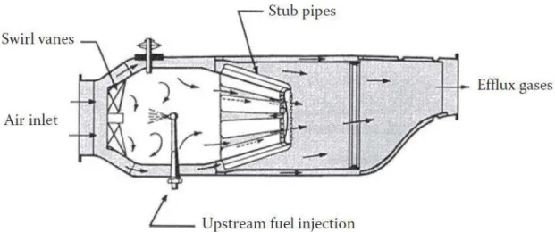
injection was unanimity. But the machines, like the German JUMO 004 (
Figure 1
) or the British Metrovik, had problemwith soot impregnating the fuel atomizer and overcooking of the fuel feed arm. In less than five years a better understanding of non-premixed combustion was achieved and by augmenting the diffusion of the air/fuel mixture with the application of a swirller, there was no more need of long residence time. It is interesting to notice how the turbomachinery, and moreover the combustor, advances together with the engineering knowledge.
17
Another interesting point is how, in the last 20 years, the combustion modes has been migrated from high power diffusive to lean premixed, most because of emissions and turbine inlet temperature control. This shows that, regardless of 70 years of evolution, there is still space for optimization inside turbomachinery combustors.Combustors Design Basics
As stated by (Lefevbre, et al.), “When good aerodynamic design is allied to a matching fuel-injection system, a
trouble-free combustor requiring only nominal development is virtually assured”. Being more direct, a good design of combustor is granted by the coupling of its principal physics, but the design optimizations is only achieved by experimental testing. There is no analytical model or commercially available software, no matter how advanced, which can estimate the performance of a combustion chamber with acceptable precision. It does not mean though, that one cannot use these tools to locally refine its virtual design, reducing the need for latter experimentation.
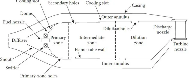
Independent of how innovative a combustor chamber can be, some components will be always present in order to transfer and accelerate the flow between compressor and turbine. These “parts” of the design and its function are listed below:
Diffuser: In order to reduce the pressure loss due to heat transfer to the flowing gas, the compressor outlet velocity must be reduced to a magnitude of 30m/s in general. This is obtained by smoothly enlarging the discharge area by the means of a diffuser
Flame tube: To contain the flame and allow discrete areas of air injection into the flame area, an internal surface is used. The flame tube is directed coupled with the diffuser in one end, and to the turbine nozzle in the other end. The flame tube has to be well cooled to withstand the hot gases from the combustion
Combustion Zones: As the temperature rise is limited by the material resistance in the turbine blades, the air/fuel ratio inside the combustor is very low, in fact, lower than the flammability limits of most fuels. So the combustion chamber has to be segmented in relation to air/fuel mixtures, creating a flame zone, a dilution zone and an intermediary zone.
Flame stabilizer: Aerodynamics devices have to be inserted in the design in order to anchor the flame in the so
called primary zone or flame zone, where almost all the combustion must take place. This is achieved by creating a recirculation area through different types of air injection. The most common solution is a Swirler, but the same recirculation effect can be developed only by arranging the air injection holes in the flame tube. Fuel injection and ignition: The fuel must be injected in the combustor in a well-atomized form, to obtain a
constant and fast burning process. This is normally achieved by flow through a small orifice under high pressure, but a variety of other devices and strategies can be used.
18
Figure 2 – Illustration of basic structures in the design of a turbomachinery combustor. (Poinsot, 2012)
The performance requirements of a modern combustor can be resumed as:
High combustion efficiency, as well as low direct emissions;
Reliable and smooth ignition, especially in case of flameout;
Flame stability over a wide pressure and load range;
Do not present pressure pulsations or others transient effects of combustion instability;
Durability with maintainability;
Multi-fuel capability.
Microturbine Combustor Requirements
As previously stated, the goal of this work is to design a biogas optimized microturbine gas combustor. This fact itself imposes a series of restrictions and pre-requisites in the chamber dimensions and attributes. For instance, the compressor and turbine for the systems have radial flow been diffused by volutes, which already acts as diffusers for the flow. More than that, the inlet and outlet geometry of the combustor are already defined by the turbo system.
In order to ease the manufacturing process, reducing the costs of the microturbine assembly, a silo tubular chamber was the only practical choice. Any kind of Can, Tuboannular or Annular topology would implicate in an aggregate cost that would make the whole system economically unfeasible. The manufacturing will consist in the rolling of stainless steel sheets, followed by knitting by welding. All the injection and wall cooling geometry will be assessed only by flame tube drilling. The author comprehend that this simplistic solution may not give the performance initially intended, but there is no engineering solution decoupled from economical limitations, and so is defined the design challenge of this work. An
19
Figure 3 – Initial CAD model for microturbine assembly.
Biogas Combustor Requirements
One of the central parameters to combustion design is the equivalence ratio from the fuel injection to the gas dilution zone. All combustor have a lean blowout limit that must be respected throughout the load range of the turbomachinery. This is the main factor that makes the alternative engines and water boilers conversion to biogas prone to failure.
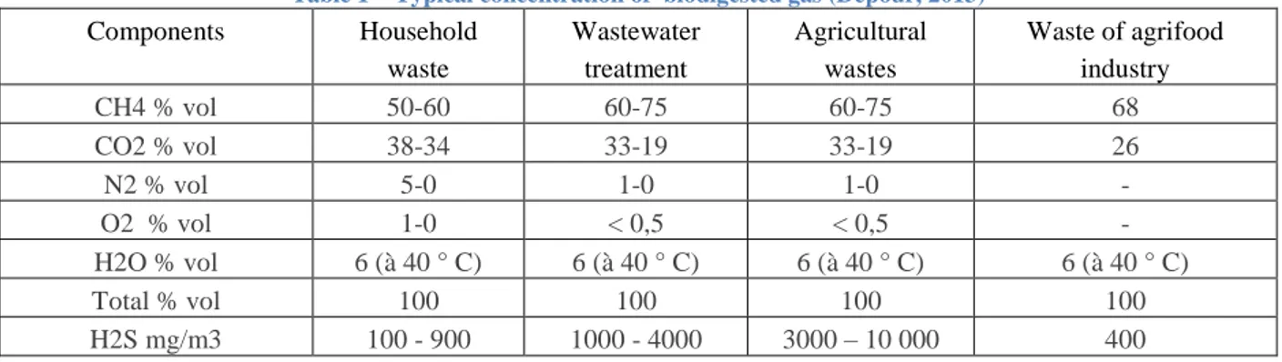
Essentially, biogas is a mixture of stable gases with combustible gases, as it can be seen in
Table 1
. What this means is that one can design a combustor for a type of biogas by changing the lean blowout limit according to the gas composition, as long as this composition is not inferior to the limit itself. That is the methodology used in this work and presented in the results section. There were other challenges in biogas burning, as industrial filtering of sulfides, but they were already solved.Table 1 – Typical concentration of biodigested gas (Depour, 2013)
Components Household
waste
Wastewater treatment
Agricultural wastes
Waste of agrifood industry
CH4 % vol 50-60 60-75 60-75 68
CO2 % vol 38-34 33-19 33-19 26
N2 % vol 5-0 1-0 1-0 -
O2 % vol 1-0 < 0,5 < 0,5 -
H2O % vol 6 (à 40 ° C) 6 (à 40 ° C) 6 (à 40 ° C) 6 (à 40 ° C)
Total % vol 100 100 100 100
20
3.
Literature Review
To characterize the methodological steps of this work, the literature is revised in the same order followed by the author in order to achieve the results presented here. This means that first analyses of the state of the art in biogas combustion in gas turbines is presented, than the analytical design theory is discussed, followed by a review of the computational models used in the multi-physical optimization of the design.
Biogas research in gas turbines
As biofuels gain space in the industrial community for its advantages regarding environmental and emissions performance, the research studies from experimental and numerical point of view began to achieve recognition and importance.
An extensive review of possibly all kinds of bio-fuels applications and researches in gas turbines was made by (Gupta, et al., 2010). The review includes liquid fuels as biodiesels, biomethanol and bioethanol but focus will be given in the biogas applications. The author concluded that:
(Ganesh A, 2001) states about the high availability of biomass in the form of cellulose derived in agricultural based economies, which could be biodigested or gasified in order to obtain biogas. An estimative of 10000MW of thermal power is presented for India, as an example.
(Rodrigues M, 2007) shows the advantages of gasification, which produce syngas with contents of 22-32% of Hydrogen. Despite this process consumes more heat in comparison with biochemical digestion, hydrogen has a very high burning speed that can attenuate the flame instabilities that comes with the burning of a leaner gas.
(Visser WPJ, 2008) presents simulations of power compromising in biogas usage that comes from its low heating value. Solutions like using two separate set of compressor, one for air and other for the biogas, or injection at compressor inlet are studied. The power loss can be from 15 to 40% according to the fuel chemical content.
Circulating fluidized bed gasifiers are presented by (Chen G, 2004) as a solution for producing higher heating value biogas in larger rates with relative compacted system. This system is relatively flexible in relation to biomass origin and form factor, minimizing preprocessing costs.
An inverted cyclone gasifier was studied by (Syred C, 2004) to produce large rates of biogas optimizing ash and particulate separation. Other advantages would be the robustness and simplicity of the system that does not require and inert material maintenance.
(Adouane B, 2002) presents design steps concerning NOx emission, modeling and experimental validation of a low heat value combustor of high power output. The combustor has good efficiency working with 2.5 to 4.0 MJ/m³ gases and pressures from 3 to 8 Bar.
A discussion of the challenges imposed by biogas content variation due to biomass feedstock composition is presented by (Richards GA, 2001). The content variation can cause instabilities in the flame that lead to greater emissions. Premix injection can be used to counter that but effects as flashback, auto ignition and lean blowout can occur.
The integration of a gasifier feeded by heat from the exhaust of an externally fired gas turbine is studied by (Kautz M, 2007). Achievement of high efficiencies due to energy recuperation and the flexibility of the externally fired combustor can justify the extra cost of the heat exchanger.
21
If the air for the gasifier is bleed from the compressor, generally it means that a higher compression load must be used in comparison with the design point. This fact diminishes the power output and of the system. The injection of steam to allow lower temperatures and grater flow energy, thus maintaining roughly the same power for biogas operation as for Natural Gas operation was demonstrated by (A, 1995).(Jager BD, 2007) has evaluated the other effects of steam injection, mostly the advantages in NOx emissions. The research showed experimentally that the emissions are reduced by two principal factors: lowering of flame temperatures and decreasing in flame speeds.
The gas characteristics compiled in the review made by (Gupta, et al., 2010). are displayed in Table 2. Although his text is from 2010, it shows that mostly of the studies are theoretical and feasibility analyses of the biogas usage. The experimental ones focus on modifications of existing designs and its subsystems in order to convert the biogas. Only one attempts to redesign the entire combustor for Biogas. This situation perpetuates today with exception of the following works.
Table 2 – Combustion properties of Syngas in relation to other conventional fuels (adapted from (Gupta, et al., 2010))
22
Figure 4 – Radio controlled model turbine
Figure 5 – Wireframe model of tuboannular combustor (adapted from (Chen, 210))
23
Another problem clearly showed by the calculation is the increase in flame temperature by prompting substituting a liquid fuel for the Low Heat Value (LVH) gas. Figure 6 is a plot of the liner temperatures for different concentrations of methane. The hotter flame can change the flow field of the combustor, resulting in flame concentration near the liner, which can be a destructive characteristic.Figure 6 – Liner temperature for methane (a) 100%, (b) 90%, (c) 80%, (d) 70% (adapted from (Chen, 210))
(Maria Cristina Cameretti, 2013) performed a more extensive study focusing in primary and pilot fuel inlet modifications and exhaust gas recirculation (EGR) configurations to enable operation of a 110kW microturbine system with biofuels. The work was done in a comparative manner, using a 65% methane to 35% carbon dioxide biogas in comparison with pure methane and using Ethanol in comparison to kerosene. First a thermokinectic model is applied to evaluate power output, thermal efficiency and NOx emission with different external EGR ratios. This configuration allows the achievement of near flameless combustion, with lower flame temperature and smothers flame gradients, near achieving a zero NOx emission state. As a setback, it comes with the cost of thermal efficiency and power output, mostly because of the higher temperature and flow in the compressor and less heat exchange in the recuperator.
24
Figure 7- Section view of the combustor chamber (adapted from (Maria Cristina Cameretti, 2013))Focusing in the gaseous part of the study, the authors try to maintain the same power output, which ended in a 235% increase in mass flow rate of Biogas in comparison with Methane. Despite that, other flow and operation parameters of the microturbine were the same. Figure 8shows the methane distribution on the injection region of the two cases solved. As expected the concentration field is roughly the same. The main changes are in flame maximum temperature and carbon monoxide emissions, due to the greater concentration of carbon dioxide in the mixture.
The literature connotes to the following points:
Biogas application in gas turbines is financial feasible if can be easily transported or generated onsite;
Most of the industrial large scale gas turbines can accept blending of biogas with natural gas or liquid fuels, if the biogas was filtered and dried;
For direct replacement of liquid fuel for biogas the entire combustion chamber must be redesigned;
For directed replacement of natural gas for biogas the injection system must be changed and the turbo-system
25
Figure 8 – Section plot of mole fraction concentration of methane in biogas redesigned injection systems (adapted from (Maria
26
4.
Combustor analytical design
When referring to analytical design of the combustor, this work covers the steps that can be used without need to computational assistance, to obtain physical and dimensional parameters of the combustor. Most of the formulas and equations have been extensively studied and tested through means of mathematical manipulation and experimentation.
As mentioned, the geometry and physical scale of all combustors are well restricted to compressor outlet and turbine inlet. This is not different for the microturbine used here as design base. The revision presented here will cover only the design steps that can be used to define geometries that are not already restricted by turbocompressor compliances. All the equations were adapted from (Lefevbre, et al., 2010).
Combustion Chamber and Liner Diameter
As a first design point to the entire chamber, one must define its diameter. This is achieved by a compromise between aerodynamic and combustion performance. To increase the reaction in the flame, turbulence and velocity are always a
good solution. To generate this conditions the air injection holes in the flame tube must work with a relative large ΔPL,
which augments the overall pressure loss from compressor outlet to turbine inlet, bringing the assembly efficiency down.
For practical application, the pressure loss must not be greater than 5%, so the chamber diameter is defined by the overall pressure loss, as can be seen in the
Eq.
below:
Eq. 1: Combustor reference area
Where:
Aref = Cross sectional area of the combustor in absence of the liner
R = gas constant, 286.9 N ∗ m kg ∗ K⁄ 𝑚̇ = air mass flow rate
T = combustor inlet temperature P = combustor inlet pressure
Δ𝑃− = pressure difference between combustor inlet and outlet
r = dynamic pressure reference value
In order to achieve an optimized ΔPL in reference to the flow in the combustion zone, and to obtain an optimized
diameter to the liner, the ratio of the liner per chamber area can be derived by
Eq. 2
:Eq. 2: Combustor area ratio
Where:
27
𝑚̇ = ratio of primary airflow to total airflowλ = diffuser pressure-loss coefficient
Δ𝑃− = pressure difference between combustor inlet and outlet
r = dynamic pressure reference value
Primary and secondary flow
The flow entering the liner will govern the primary and secondary combustion zones, as well as the dilution process. Hole area and pressure drop are the most important parameters that define the injection through the hole, but another aerodynamics can change significantly the flow direction and behavior, like the presence of swirl and local pressure disturbances. The mass flow can be expressed as shown in
Eq. 3
:Eq. 3: Hole mass flow
Where:
C𝐷 = discharge coefficient
Ah.geom = hole area
P = total ambient pressure ρ = density at combustor inlet p = static pressure at jet stream
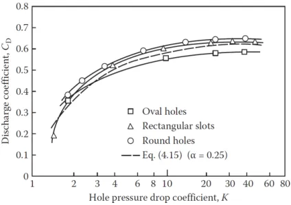
The discharge coefficient was extensively studied by (Kaddah, 1964), being best described by
Eq. 5
, which is in good accordance with experimental data, as shown inFigure 9
:Eq. 4: Hole discharge coefficient
Where:
C𝐷 = discharge coefficient
K = hole pressure drop coefficient
28
Figure 9 – Variation of discharge coefficient wit hole pressure drop coefficient
In a typical tubular chamber, multiple radially distributed holes are used to fully accomplish the air injection and mixing. Jet penetration is altered by multijet presence, because one stream can be blocking the others. The penetration of multiple jets was studied by (Sridhara, 1967) and (Norster, 1964), suggesting the following equation (
Eq. 5
) for the radial reach of the streams:Eq. 5: Hole radial penetration
Where:
Ymax = Maximum radial penetration of a multijet circular hole inside a tubular combustor
J = momentum-flux ratio d = jet diameter
𝑚̇ = total gas mass flow rate 𝑚̇ = jet air mass flow rate
As a rule of thumb, a circular jet in a tubular combustor must reach between 60% and 70% of the radial length of the liner. With these equations and the mass flow chemical requirements for the primary and secondary reaction zones, one can chose optimally the geometry and dimensions of the first two combustion zones.
Dilution flow
For the dilution zone, mixing parameters must be studied together with the aerodynamic ones, because of the influence in the temperature traverse quality of the turbine inlet. The main preoccupation here is to impede the formation of hot clusters of gas. Further refining can be done experimentally to achieve the desired radial distribution of temperature, matching it to the blade refrigeration capabilities.
To minimize the temperature gradient of the combustor outlet, the dilution process must be designed to maximize jet penetration and distribution. This is made by coupling
Eq. 5
to the Cranfield (Eq. 6
) equation below:Eq. 6: Cranfield design equation
29
n = number of dilution holesdj = jet diameter of dilution holes
𝑚̇ = jet air mass flow rate for dilution holes T = combustor inlet temperature
P = combustor inlet pressure
Δ𝑃𝐿 = pressure drop available in the liner
By setting Ymax to 0.33DL, the jet optimum diameter can be found and used to get related number of holes. The physical
30
5.
Numerical Models Theory
In this section, the physics knowledge inside the computational models used in this work is reviewed. The discussion is focused in the numerical modeling of the Thermal, Fluid, Chemical and Combustion characteristics, beyond of its basic principles. The author believes that the potential reader for this work already has an advanced understanding of the physics itself.
In general, all the rules and models explanation found in this section can be further investigated at (Ansys,Inc, November 2013). In an attempt to ease the understanding of the multiphysics solution process, the knowledge will be revised in the following order:
-Non-premixed Combustion;
-Heat Generation and Transfer;
-Fluid Flow;
Non-premixed Combustion
Whenever the oxidizer and fuel enter the reaction zone in separated streams, a non-premixed burning situation is develop. Contrary to premixed systems, in which reactants are mixed at the molecular level before combustion, the time scale of the non-premixed system is defined by the species diffusion processes, instead of the burning velocity.
Most of the initial developments in turbomachinery combustor uses this kind of mechanism. Only recently premixed swirller and burner are being used in industrial generators because of the lower peak temperatures achieved, that contributes to lower NOx emissions. Examples of non-premixed industrial combustion equipment’s include diesel internal-combustion engines, solid powder pulverized furnaces and wood fires.
Mathematically, observing some limit conditions, the thermochemistry of non-premixed combustion can be described by a parameter called mixture fraction ( ). It represents the mass fraction of fuel after its injection in the chamber. Its importance comes from making possible a high traceability of burnt and unburnt mass fractions of the species involved in the combustion. Using the mass fraction to balance the equations is interesting because of the conservation of elements in the combustion reaction. This makes a scalar amount that is preserved, and its coupled transport equation has no source term, easing the solution.
31
Mixture Fraction Definition
The non-premixed modeling is centered in a group of assumptions that simplify the solution, being the most important that the local and actual state of the gases is related to the mixture fraction, defined by:
Eq. 7: Mixture fraction definition
Where:
= value of the mixture fraction
Zi = elemental mass fraction for element i
Zi,ox = elemental mass fraction for element i in the oxidizer stream
Zi,fuel = elemental mass fraction for element i in the fuel stream
For one fuel stream, if all species have equal diffusion coefficients, is the same for all the species, and it becomes the elemental mass fraction of fuel injected by this stream. Independent of how many streams of fuel and oxidizer, the sum of its relative mixture fraction always equals to 1.
This characteristic is the first requisition for the non-premixed model. In order for the diffusion coefficients be the same for all species, the flow must be turbulent, which is a normal condition inside turbomachinery burners where Reynolds numbers of 105 are achieved. If the flow is in near laminar conditions, the turbulent convection can be overwhelmed by the molecular diffusion, and this approach becomes invalid.
If the equal diffusivity can be applied, the species equation can be substituted by a single mixture fraction equation, and the reaction source term becomes null because of the conservation of elements in chemical reactions. Therefore, the density averaged Frave mixture equation is:
Eq. 8: Conservation equation rearranged for density averaged mixture fraction
Where:
̅= density averaged mixture fraction µt = turbulent viscosity
µl = laminar viscosity ρ = local density
̅ = velocity vector
𝜎 = viscosity weighting constant
Sm = source term due to transfer of mass into the gas phase from liquid fuel droplets or reacting particles
The mixture fraction can be related to the equivalence ratio ( ) by the equation below. This relation can be used to plot fields, informing where the mixture is rich and where it becomes lean.
= +
Eq. 9: Relation of mixture fraction and equivalence ratio
32
= mixture fractionr = turbulent viscosity = equivalence ratio
Another advantage of mixture fraction modeling is the close relationship between its value and the density, temperature and species mass fraction. For a non-adiabatic system, where heat is transferred through radiation, walls, etc., the instantaneous value of these parameters depends solely on the mixture fraction and enthalpy (effects of heat gain or loss) values, reducing the mathematical complexity of the calculation.
Probability Density Function for Turbulence Chemistry interaction
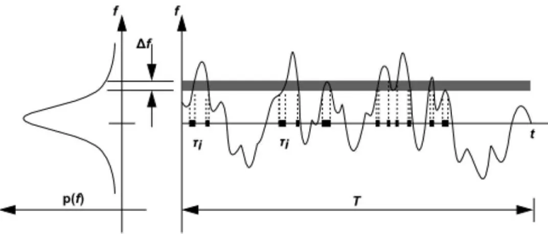
In order to translate the instantaneous values of the mixture fraction model scalars into averaged values that can be interpreted and used for convergence of steady-state situations, a model to account for the fluid-chemistry iteration must be used. In this work, a self-check routine based on the assumed-shape Probability Density Function is used to regulate
the time-scale in the average composition. Denoted by , the function is written as:
Eq. 10: PDF general definition
Where:
= Probability Density Function T = time scale
𝜏 = amount of time that spends in the Δ range
The PDF can be interpreted by the amount of time a scalar stays in a defined range of value, as can be seen in Figure 10. In the right side we have a plot during a time and in the left side a distribution of along the range of . The hard
fact here is that the is unknown in the beginning of the solving process, being modeled as a mathematical function
that approximates to experimental PDF shapes measured in the bibliography, thus the assumed shape term.
Figure 10 – Graphical demonstration of averaging technique used in PDF
33
Eq. 11: PDF formulation for 𝒇 and 𝒇′𝟐
Eq. 12: Alpha mixture fraction subfunction
Eq. 13: Beta mixture fraction subfunction
Where:
= Probability Density Function ̅= density averaged mixture fraction
′
̅̅̅̅= density averaged mixture fraction variance 𝜏 = amount of time that spends in the Δ range
With these correlations, only by calculating the mixture fraction and its variance throughout the mesh, according to the boundary and start, conditions the solver can compute the local instantaneous values of temperature, density and species mass fractions, assembly the PDF, and return the mean values of temperature, density and mass fractions.
Enthalpy variations due to heat transfer can impact the equilibrium equations, affecting temperature and species formation, consequently changing the scalars calculation from mixture fraction. Basically, the parameters will be no longer related only to , but to too. Solving this joint PDF is not practical in engineering applications, so a simplification is made. If the heat losses do not impact the turbulent enthalpy fluctuations, the PDF can be described as:
Eq. 14: Enthalpy corrected PDF definition
Where:
, = Probability Density Function corrected by enthalpy levels
= standard Probability Density Function ̅= mean enthalpy level
= local enthalpy of mixture
34
Figure 11 – Representation of the Probability Density Function for a scalar parameter in relation to Mixture Fraction, its
variance and the multi-level enthalpy correction.
For the simulation proposed in this work, and practically all the turbomachinery combustors, thermal loss is under 5%. The gases usually take less 0.1s to go from inlet to outlet. Although elevated temperatures are achieved, the timescale is very short and there is no relevant heat transferred to the casing or ambient medium. This grants the fulfillment of the requisition. Mathematically, the only change is that the modeled transport equation has to be solved in order to get the instantaneous values of temperature, density and species mass fraction. The resultant PDF and enthalpy levels can be preprocessed and organized in a look-up table, saving a great amount in computational time during the actual solving.
Flamelet Models Theory
35
Figure 12 – Schematic representation of flamelet model theory.
The scalars are mapped in relation to the mixture fraction along the one-dimensional axle, henceforth being described by itself and the flow strain rate, which is obviously computationally favorable. The strain rate in a laminar counter flow flame is given by the ratio between the relative speed of the streams by the double of the jet nozzles distance. In order to get a better coupling of the equations, the strain rate is used indirectly as an input of the scalar dissipation, that depends itself of the mixture fraction, changing along the flamelet axle, as can be seen in the equation
Eq. 15
:Eq. 15: Flamelet scalar dissipation
Where:
= scalar dissipation 𝑎 = characteristic strain rate
= stoichmetric mixture fraction
𝑐− = inverse complementary error function
is used to measure the stoichmetric imbalance and can be interpreted as the inverse of the diffusion time. Flame
quenching is achieved when reaches a superior limit. If tends to zero, the flame is extinguished due to36
Heat Generation and Transfer
Thermal energy is present at every substance in the form of temperature. Whenever two different volumes with different temperatures interact, there will be heat transfer. Moreover, in this application, heat is inserted in the system by the combustion reaction, generating heat by the reaction of substances. In this chapter the modeling of these physical phenomena will be explained.
Energy Equation
To solve the energy flux in each volume cell, the energy equation is implemented as:
Eq. 16: Energy conservation formula
and
Eq. 17: Total energy simplified equation
Where:
𝑘 = effective conductivity, sum of laminar, turbulent and radiation conduction ̅ = diffusion flux of species j
ℎ = enthalpy of species j 𝜌 = local density
= local total pressure = velocity amplitude ℎ = local sensible enthalpy
= local temperature
𝜏⃗̅ = viscous dissipation tensor
ℎ= chemical reaction and/or other sources heat source
In the left side of the equation, the first term represents the time variation of the total energy of the cell. The second term describes the changes in energy due to translational or rotational movement.
Each term inside the parenthesis in the right side of the equation is coupled with a different kind of heat mechanism. The first one gives the effective conduction of heat, a sum of turbulent and conventional conduction factors. The middle term is related with heat transferred by the diffusion of species with different enthalpy. The last one describes the viscous dissipation due to shear in the fluid.
The term ℎ is a universal source term that would depend on the physics being solved and boundary conditions. For example, as radiation depends in cell to cell calculations, it is solved in a parallel model and included in the equation by this source term. The same goes for the heat generation by combustion reaction or for heat transfer from walls.
37
Eq. 18: Non-adiabatic energy conservationWhere:
𝑘 = turbulent conductivity
= mass fraction averaged enthalpy sum for all species 𝜌 = local density
𝑐𝑝 = specific heat for constant pressure
ℎ= chemical reaction and/or other sources heat source
As turbulence is a prerequisite of the model and the Lewis number is near unity, the conduction and diffusion terms are combined in the first right hand term. The total enthalpy is a sum of each individual enthalpy of the species being calculated, balanced by its mass fraction.
For the combustion problem, the flame temperature can achieve 2500K, where radiation stands out as an important part of the heat exchange. Being a complex physical problem with a variety of models available to solve the same situation, it will be discussed separately.
Radiation Modeling
Radiation can be interpreted as electromagnetic waves interaction between atoms. It is a mechanism of heat transfer that depends to the fourth order of temperature level. As in combustion high levels of temperature flames are achieved, radiation is very present. For instance, the liner wall temperature rise is almost entirely due to this effect, as long as the film cooling mechanism of the wall is working as designed.
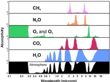
Different from solids or fluids, the emission and absorption of radiation in gases does not occur in the entire wavelength spectrum. Only in narrow frequency strips a gas has wave interaction, although there are a large number of this strips, as it can be seen in the
Figure 13
.Figure 13 – Absorptivity spectrum of gases, showing the narrow strips of absorption (Sciences, 2014)
38
The Weighted-Sum-of-Gray-Gases Model
Therefore called WSGGM, this model is a time saving compromise between assuming fixed coefficients and implementing all the coefficients for all bands for all species in the simulation. Very similar to other lookup tables used in the non-premixed model, it uses experimental information about each species and arrives at the total coefficients by a sum weighted by the gas partial pressure in the mixture. Wherever waveband the coefficients are zero, the partial term of the sum assumes a null value, so the resultant coefficient value is a single beam composed by the partial values of all the narrow beams. The emissivity and absorptivity are corrected by pressure and temperature too, again using interpolation of experimental data. Mathematically, the WSGGM can be described as:
Eq. 19: Emissivity WSGGM formulation
Where, for each ith simulated gas:
𝑎𝜀, = weighting factor
𝑘 = absorption coefficient
= sum of partial pressures for all species = radiation path length
= temperature
The same goes for the absorptivity, but again for computational saving purposes, e=a, which is valid whenever the medium is optically thick. For the absorption coefficient, in our case where the path length is big enough, the calculation is done using the emissivity from the WSGGM, according to the expression:
Eq. 20: Absorptivity WSGGM formulation
Where:
𝑎 = absorption coefficient 𝜀 = emissivity
= radiation path length
Radiation Model Selection
Once the transmission coefficients calculation is done, the transfer equation for the radiative exchange can be composed and solved. Regardless of the medium, radiation can be absorbed, emitted or scattered by it. Generally speaking, the process can be mathematically described by the equation:
Eq. 21: Radiation transfer equation
Where:
39
⃗ = direction vector⃗′ = scattering direction vector 𝑎 = absorption coefficient 𝜎 = scattering coefficient = radiation path length n = refractive index
𝜎 = Stefan-Boltzmann constant
= radiation intensity = local temperature 𝜙 = phase function Ω′= solid angle
Each of the available models will approach the solution of this equation with different simplifications or discretization, requiring more computational time as the solution comes to solving of the complete equation. The radiation models in ANSYS platforms have been extensively tested and its performance was scaled in relevance to physical attributes of different case simulations, like optical thickness, path length, expected pressure and temperature, and so on. Considering the distance from the flame surface to the wall as being ¼ of the diameter of the liner tube, and the cylindrical geometry
of the liner tube itself, the situation simulated constitutes an optical and physical thick problem, achieving αL and s of 10² magnitudes. This information, together with the possible temperatures achieved by the flame, is enough to select the Rosseland model as first option.
Rosseland Model (RM)
As the majority of radiation models, RM describes the intensity of the phenomena by expanding it in an orthogonal series of harmonics in spherical form. Using the four first terms of the series, the radiation thermal flux is determined by equation:
Eq. 22: Radiation flux
Where:
= radiation flux 𝑎 = absorption coefficient 𝜎 = scattering coefficient
𝐶 = linear-anisotropic phase function coefficient = incident radiation
Because of RM assumptions, G can be simplified as the black body intensity at gas temperature. Thus, the thermal flux becomes:
Eq. 23: Rosseland black body radiation
and
Eq. 24: Rosseland coefficient
40
= radiation flux𝑎 = absorption coefficient 𝜎 = scattering coefficient n = refractive index
𝜎 = Stefan-Boltzmann constant
𝐶 = linear-anisotropic phase function coefficient = temperature
This is very interesting by the computational point of view, because the equation is composed in the same form as the Fourier conduction law, and can therefore be embedded in the energy equation as radioactive conductivity, simplifying the solution, as:
41
Fluid flow
To complete the multiphysical simulation process of the combustion chamber, after discussing the energy and the mixture fraction conservation equations, only the mathematics involving mass and momentum transfer needs to be added to the solution. By solving this set of equations, the gas is modeled as fluid and the results characterize its final flow, by outputting pressure and velocity fields. The general form of mass and momentum conservation equations, respectively, are:
Eq. 25: Mass conservation equation
and
Eq. 26: Momentum conservation equation
Where:
𝜌 = local density = local total pressure ⃗ = velocity vector ⃗ = gravity vector ⃗ = external body forces 𝜏⃗̅ = stress tensor
= mass source due to interphase state changes
In
Eq. 25
, Sm can be used to simulate mass transfer between continuous and discrete phase, as well as any other masssources. In
Eq. 26
, F is any external force, and is used too to describe other momentum sources, like porous media and so on. 𝜏⃗̅ is the viscous stress tensor, here defined by:Eq. 27: Viscous stress tensor
Where:
⃗ = velocity vector = unit tensor
𝜇 = molecular viscosity
42
Turbulence Modeling
As mentioned before, non-premixed burning in turbomachinery combustors is a highly turbulent phenomenon. A robust model to describe the turbulence interference in the mass and momentum equation is a pre-requisite to simulate combustion in such equipment. Moreover, whenever rotation or swirling is present, most of the less expensive models have convergence problems. Like in the radiation simulation area, turbulence models have been extensively studied, constituting a research area that is ever-changing. This work will limit itself by not describing in detail all that available models. Instead, a pre-selection of the model configuration was made according to (Ansys,Inc, November 2013), and only the chosen model will be fully studied.
The platform used to the solution has more than 300 configurations of models, sub-models and sub-routines to fully cover every aspect of turbulence. Besides this fact, all the approaches consist in separating mathematically the mean value of the scalar parameters from their fluctuation, which is caused by the flow turbulence. Because of the limited computational infrastructure, a Reynolds Averaged Navier-Stokes model, based in the renormalization of the k-ε formulation, with subroutine to account for intense swirls and local Prandlt number variations. The authors recognizes that a Reynolds Stress Transport model or Large Eddy Simulation would be more suitable for the application, but previous tests with this model and several solver were not successful in both convergence and computing time.
Reynolds Averaged Navier-Stokes Models
Therefore called RANS, this formulation applies a decomposition of scalars parameters in a time-averaged value plus a fluctuating one, as can be exemplified in the velocity equation:
= ̅ + ′
Eq. 28: RANS velocity simplified formulation
Where:
= composite velocity of component i ̅ = mean velocity of component i
′ = fluctuating velocity of component i
The same principle is applied for pressure, energy or mass fraction of species. Rearranging the continuity and momentum equations into Cartesian tensor form, one can arrive at the RANS equations:
Eq. 29: RANS continuity equation
and
Eq. 30: RANS momentum equation
Where:
43
= mean velocity of i component= mean velocity of j component
= mean velocity of l component u′ = fluctuating velocity of i component u′ = fluctuating velocity of j component μ = molecular viscosity
= stress component of i in relation to j
These equations are very similar to the Navier-Stokes form, having in addition only the Reynolds stress term, in the end of
Eq. 30
and the fact that all the scalars are time averaged. All the RANS models differ only on the approach to calculate the Reynolds stress in various regions and flow situations. The selected model uses the Boussinesq approach to relate the Reynolds stresses to the mean velocity gradient, as shown inEq. 31
:Eq. 31:Boussinesq equation
Where:
𝜌 = local density
𝑥 = displacement in i direction x = displacement in j direction x = displacement in l direction
= mean velocity of i component = mean velocity of j component
= mean velocity of l component u′ = fluctuating velocity of i component u′ = fluctuating velocity of j component μ = turbulent viscosity
k = turbulent kinetic energy
= stress component of i in relation to j
The Renormalization Group k-
ε Model
Proposed by (Spalding, 1974), k-ε approach uses the transport equations for turbulence Kinect energy (k) and its dissipation rate (ε), to obtain the turbulent viscosity (µt). It is a hybrid formulation, being that k is analytically derived and
ε is experimentally composed. One of its limitations is the requirement that all the flow is fully turbulent, which in this application is granted by the minimal Reynolds of 104 magnitude. Being one of the most industrially used turbulence
model, its weakness were well documented along the years, resulting in several improvements. The RNG k-ε is a result
of these attempts, were the following capabilities were added to the standard k-ε:
Addition of a time sensitive term in the ε formulation, improving accuracy for rapidly accelerated flow; Inclusion of an analytical formula for Prandlt numbers under high-Reynolds flow, instead of the user
defined one in the standard model;
Alteration of the equation for effective viscosity for a derived differential formula that withstands low-Reynolds regimes;
Inclusion of torsion in streamlines, enhancing accuracy of swirling flows;
Better coupling with wall treatment models;
44
Eq. 32: RNG k-ε mass conservation
and
Eq. 33: RNG k-ε momentum conservation
Where:
𝜌 = local density
𝑥 = displacement in i direction x = displacement in j direction
= mean velocity of i component = mean velocity of j component
G = turbulent kinetic energy generation term due to velocity gradients Gb = turbulent kinetic energy generation term due to buoyancy
Y = compressible turbulent dilatation term 𝑎𝜀 = inverse effective Prandtl number for ε
𝑎 = inverse effective Prandtl number for k k = turbulent kinetic energy
= turbulent kinetic energy dissipation rate
μ = turbulent viscosity locally corrected by k, ε and ρ
C 𝜀, , = model constants
R𝜀 = Strained flow correction term
S𝜀 = source term for kinetic energy dissipation
S = source term for kinetic energy
As mentioned,
Eq. 31
is used to calculate de effective viscosity, than reinserted in the RANS equations. The RNG procedure arrives at the following formula:Eq. 34: Turbulent viscosity differential equation
Where:
𝜌 = local density
k = turbulent kinetic energy
= turbulent kinetic energy dissipation rate μ = local viscosity
C𝑣 = model constants
̂ = dynamic viscosity
45
Swirling modification is achieved by state function that corrects the actual value of effective viscosity, as can be seen inEq. 35
:Eq. 35: Swirl modified turbulent viscosity formulation
Where:
μ = swirl corrected local viscosity μ = swirl uncorrected local viscosity k = turbulent kinetic energy
= turbulent kinetic energy dissipation rate 𝑎 = swirl weight correction factor
Ω = pre-calculated swirl number
The RANS analogy is implemented in the energy equation as well, to account for the turbulence effect in heat transfer. The altered energy equation takes the form of:
Eq. 36: RANS energy equation
Where:
𝜌 = local density = total pressure
𝑥 = displacement in i direction x = displacement in j direction
= mean velocity of i component = mean velocity of j component T = local temperature
E = total energy
k = effective thermal conductivity Sℎ = source term for heat insertion
k = turbulent kinetic energy
(τ ) = deviatoric stress tensor
The sensible difference is the appearance of the deviatoric stress tensor and the alteration of effective thermal conductivity by the turbulence parameters, defined respectively as:
Eq. 37: Deviatoric stress tensor
and
Eq. 38: Turbulence biased thermal conductivity
46
(τ ) = deviatoric stress tensor
μ = effective viscosity 𝑥 = displacement in i direction x = displacement in j direction x = displacement in l direction
= mean velocity of l component = mean velocity of i component = mean velocity of j component 𝑎 = inverse Prandlt number
𝑐𝑝 = specific heat for constant pressure
k = effective thermal conductivity = stress component of i in relation to j
47
6.
Combustor Design
Microturbine Requirements
As previously stated, all combustors are geometrically limited by their turbomachinery annexes. Furthermore, it must achieve performance and financial goals in order to make the entire system economically viable.
Figure 14
shows the turbo-generator developed by FAHREN Inc, in which the presented design is to be installed.Figure 14 – Turbo-Generator-Compressor block
The geometry of compressor outlet and turbine inlet are well defined, so the combustor must be designed best suit this geometries. From the system operational points we can get the parameters presented in
Table 3
:Table 3 – Microturbine operational parameters
Parameter Value Unit
Compressor outlet pressure 3,00 Bar
Turbine inlet pressure 2,95 Bar
Compressor mass flow 0,350 kg/s
Fuel mass flow (methane) 0,003 kg/s
Turbine inlet maximum temperature 800 ºC
Compressor outlet temperature 250 ºC
Primary zone mass flow 0,060 kg/s
Another factor that can be discussed is the reverse flow of the combustor chamber. This design choice comes from the financial target of the entire microturbine system. The reverse flow makes possible several design strategies that minimizes the combustor cost like:
Elimination of diffuser geometry manufacturing, as the flow is decelerated by a toroid damper, before entering
the annulus;