Azimuthal decorrelations and multiple parton interactions in
þ
2
jet
and
þ
3
jet events in
p
p
collisions at
p
ffiffiffi
s
¼
1
:
96 TeV
V. M. Abazov,35B. Abbott,72B. S. Acharya,29M. Adams,48T. Adams,46G. D. Alexeev,35G. Alkhazov,39A. Alton,60,* G. Alverson,59G. A. Alves,2L. S. Ancu,34V. B. Anikeev,38M. Aoki,47M. Arov,57A. Askew,46B. A˚ sman,40 O. Atramentov,64C. Avila,8J. BackusMayes,79F. Badaud,13L. Bagby,47B. Baldin,47D. V. Bandurin,46S. Banerjee,29 E. Barberis,59P. Baringer,55J. Barreto,3J. F. Bartlett,47U. Bassler,18V. Bazterra,48S. Beale,6A. Bean,55M. Begalli,3
M. Begel,70C. Belanger-Champagne,40L. Bellantoni,47S. B. Beri,27G. Bernardi,17R. Bernhard,22I. Bertram,41 M. Besanc¸on,18R. Beuselinck,42V. A. Bezzubov,38P. C. Bhat,47V. Bhatnagar,27G. Blazey,49S. Blessing,46K. Bloom,63 A. Boehnlein,47D. Boline,69T. A. Bolton,56E. E. Boos,37G. Borissov,41T. Bose,58A. Brandt,75O. Brandt,23R. Brock,61
G. Brooijmans,67A. Bross,47D. Brown,17J. Brown,17X. B. Bu,47M. Buehler,78V. Buescher,24V. Bunichev,37 S. Burdin,41,†T. H. Burnett,79C. P. Buszello,40B. Calpas,15E. Camacho-Pe´rez,32M. A. Carrasco-Lizarraga,55 B. C. K. Casey,47H. Castilla-Valdez,32S. Chakrabarti,69D. Chakraborty,49K. M. Chan,53A. Chandra,77G. Chen,55 S. Chevalier-The´ry,18D. K. Cho,74S. W. Cho,31S. Choi,31B. Choudhary,28T. Christoudias,42S. Cihangir,47D. Claes,63 J. Clutter,55M. Cooke,47W. E. Cooper,47M. Corcoran,77F. Couderc,18M.-C. Cousinou,15A. Croc,18D. Cutts,74A. Das,44 G. Davies,42K. De,75S. J. de Jong,34E. De La Cruz-Burelo,32F. De´liot,18M. Demarteau,47R. Demina,68D. Denisov,47 S. P. Denisov,38S. Desai,47K. DeVaughan,63H. T. Diehl,47M. Diesburg,47A. Dominguez,63T. Dorland,79A. Dubey,28
L. V. Dudko,37D. Duggan,64A. Duperrin,15S. Dutt,27A. Dyshkant,49M. Eads,63D. Edmunds,61J. Ellison,45 V. D. Elvira,47Y. Enari,17H. Evans,51A. Evdokimov,70V. N. Evdokimov,38G. Facini,59T. Ferbel,68F. Fiedler,24 F. Filthaut,34W. Fisher,61H. E. Fisk,47M. Fortner,49H. Fox,41S. Fuess,47T. Gadfort,70A. Garcia-Bellido,68V. Gavrilov,36
P. Gay,13W. Geist,19W. Geng,15,61D. Gerbaudo,65C. E. Gerber,48Y. Gershtein,64G. Ginther,47,68G. Golovanov,35 A. Goussiou,79P. D. Grannis,69S. Greder,19H. Greenlee,47Z. D. Greenwood,57E. M. Gregores,4G. Grenier,20Ph. Gris,13 J.-F. Grivaz,16A. Grohsjean,18S. Gru¨nendahl,47M. W. Gru¨newald,30F. Guo,69G. Gutierrez,47P. Gutierrez,72A. Haas,67,‡ S. Hagopian,46J. Haley,59L. Han,7K. Harder,43A. Harel,68J. M. Hauptman,54J. Hays,42T. Head,43T. Hebbeker,21 D. Hedin,49H. Hegab,73A. P. Heinson,45U. Heintz,74C. Hensel,23I. Heredia-De La Cruz,32K. Herner,60M. D. Hildreth,53
R. Hirosky,78T. Hoang,46J. D. Hobbs,69B. Hoeneisen,12M. Hohlfeld,24S. Hossain,72Z. Hubacek,10,18N. Huske,17 V. Hynek,10I. Iashvili,66R. Illingworth,47A. S. Ito,47S. Jabeen,74M. Jaffre´,16S. Jain,66D. Jamin,15R. Jesik,42K. Johns,44
M. Johnson,47D. Johnston,63A. Jonckheere,47P. Jonsson,42J. Joshi,27A. Juste,47,xK. Kaadze,56E. Kajfasz,15 D. Karmanov,37P. A. Kasper,47I. Katsanos,63R. Kehoe,76S. Kermiche,15N. Khalatyan,47A. Khanov,73A. Kharchilava,66
Y. N. Kharzheev,35D. Khatidze,74M. H. Kirby,50J. M. Kohli,27A. V. Kozelov,38J. Kraus,61A. Kumar,66A. Kupco,11 T. Kurcˇa,20V. A. Kuzmin,37J. Kvita,9S. Lammers,51G. Landsberg,74P. Lebrun,20H. S. Lee,31S. W. Lee,54W. M. Lee,47
J. Lellouch,17L. Li,45Q. Z. Li,47S. M. Lietti,5J. K. Lim,31D. Lincoln,47J. Linnemann,61V. V. Lipaev,38R. Lipton,47 Y. Liu,7Z. Liu,6A. Lobodenko,39M. Lokajicek,11P. Love,41H. J. Lubatti,79R. Luna-Garcia,32,kA. L. Lyon,47 A. K. A. Maciel,2D. Mackin,77R. Madar,18R. Magan˜a-Villalba,32S. Malik,63V. L. Malyshev,35Y. Maravin,56
J. Martı´nez-Ortega,32R. McCarthy,69C. L. McGivern,55M. M. Meijer,34A. Melnitchouk,62D. Menezes,49 P. G. Mercadante,4M. Merkin,37A. Meyer,21J. Meyer,23F. Miconi,19N. K. Mondal,29G. S. Muanza,15M. Mulhearn,78
E. Nagy,15M. Naimuddin,28M. Narain,74R. Nayyar,28H. A. Neal,60J. P. Negret,8P. Neustroev,39S. F. Novaes,5 T. Nunnemann,25G. Obrant,39J. Orduna,32N. Osman,42J. Osta,53G. J. Otero y Garzo´n,1M. Owen,43M. Padilla,45
M. Pangilinan,74N. Parashar,52V. Parihar,74S. K. Park,31J. Parsons,67R. Partridge,74,‡N. Parua,51A. Patwa,70 B. Penning,47M. Perfilov,37K. Peters,43Y. Peters,43G. Petrillo,68P. Pe´troff,16R. Piegaia,1J. Piper,61M.-A. Pleier,70
P. L. M. Podesta-Lerma,32,{V. M. Podstavkov,47M.-E. Pol,2P. Polozov,36A. V. Popov,38M. Prewitt,77D. Price,51 S. Protopopescu,70J. Qian,60A. Quadt,23B. Quinn,62M. S. Rangel,2K. Ranjan,28P. N. Ratoff,41I. Razumov,38 P. Renkel,76M. Rijssenbeek,69I. Ripp-Baudot,19F. Rizatdinova,73M. Rominsky,47C. Royon,18P. Rubinov,47R. Ruchti,53 G. Safronov,36G. Sajot,14A. Sa´nchez-Herna´ndez,32M. P. Sanders,25B. Sanghi,47A. S. Santos,5G. Savage,47L. Sawyer,57
T. Scanlon,42R. D. Schamberger,69Y. Scheglov,39H. Schellman,50T. Schliephake,26S. Schlobohm,79 C. Schwanenberger,43R. Schwienhorst,61J. Sekaric,55H. Severini,72E. Shabalina,23V. Shary,18A. A. Shchukin,38 R. K. Shivpuri,28V. Simak,10V. Sirotenko,47N. B. Skachkov,35P. Skubic,72P. Slattery,68D. Smirnov,53K. J. Smith,66
G. R. Snow,63J. Snow,71S. Snyder,70S. So¨ldner-Rembold,43L. Sonnenschein,21A. Sopczak,41M. Sosebee,75 K. Soustruznik,9B. Spurlock,75J. Stark,14V. Stolin,36D. A. Stoyanova,38M. Strauss,72D. Strom,48L. Stutte,47L. Suter,43
N. Varelas,48E. W. Varnes,44I. A. Vasilyev,38P. Verdier,20A. Verkheev,35L. S. Vertogradov,35M. Verzocchi,47 M. Vesterinen,43D. Vilanova,18P. Vint,42P. Vokac,10H. D. Wahl,46M. H. L. S. Wang,68J. Warchol,53G. Watts,79
M. Wayne,53M. Weber,47,**L. Welty-Rieger,50A. White,75D. Wicke,26M. R. J. Williams,41G. W. Wilson,55 S. J. Wimpenny,45M. Wobisch,57D. R. Wood,59T. R. Wyatt,43Y. Xie,47C. Xu,60S. Yacoob,50R. Yamada,47W.-C. Yang,43
T. Yasuda,47Y. A. Yatsunenko,35Z. Ye,47H. Yin,47K. Yip,70S. W. Youn,47J. Yu,75S. Zelitch,78T. Zhao,79B. Zhou,60 J. Zhu,60M. Zielinski,68D. Zieminska,51and L. Zivkovic74
(D0 Collaboration)
1
Universidad de Buenos Aires, Buenos Aires, Argentina
2LAFEX, Centro Brasileiro de Pesquisas Fı´sicas, Rio de Janeiro, Brazil 3
Universidade do Estado do Rio de Janeiro, Rio de Janeiro, Brazil
4Universidade Federal do ABC, Santo Andre´, Brazil 5
Instituto de Fı´sica Teo´rica, Universidade Estadual Paulista, Sa˜o Paulo, Brazil
6Simon Fraser University, Vancouver, British Columbia, and York University, Toronto, Ontario, Canada 7University of Science and Technology of China, Hefei, People’s Republic of China
8Universidad de los Andes, Bogota´, Colombia
9Charles University, Faculty of Mathematics and Physics, Center for Particle Physics, Prague, Czech Republic 10
Czech Technical University in Prague, Prague, Czech Republic
11Center for Particle Physics, Institute of Physics, Academy of Sciences of the Czech Republic, Prague, Czech Republic 12
Universidad San Francisco de Quito, Quito, Ecuador
13LPC, Universite´ Blaise Pascal, and CNRS/IN2P3, Clermont, France 14
LPSC, Universite´ Joseph Fourier Grenoble 1, CNRS/IN2P3, and Institut National Polytechnique de Grenoble, Grenoble, France
15CPPM, Aix-Marseille Universite´, and CNRS/IN2P3, Marseille, France 16LAL, Universite´ Paris-Sud, and CNRS/IN2P3, Orsay, France 17LPNHE, Universite´s Paris VI and VII, and CNRS/IN2P3, Paris, France
18CEA, Irfu, SPP, Saclay, France 19
IPHC, Universite´ de Strasbourg, and CNRS/IN2P3, Strasbourg, France
20IPNL, Universite´ Lyon 1, CNRS/IN2P3, Villeurbanne, France and Universite´ de Lyon, Lyon, France 21
III. Physikalisches Institut A, RWTH Aachen University, Aachen, Germany
22Physikalisches Institut, Universita¨t Freiburg, Freiburg, Germany
23II. Physikalisches Institut, Georg-August-Universita¨t Go¨ttingen, Go¨ttingen, Germany 24Institut fu¨r Physik, Universita¨t Mainz, Mainz, Germany
25Ludwig-Maximilians-Universita¨t Mu¨nchen, Mu¨nchen, Germany 26
Fachbereich Physik, Bergische Universita¨t Wuppertal, Wuppertal, Germany
27Panjab University, Chandigarh, India 28
Delhi University, Delhi, India
29Tata Institute of Fundamental Research, Mumbai, India 30
University College Dublin, Dublin, Ireland
31Korea Detector Laboratory, Korea University, Seoul, Korea 32CINVESTAV, Mexico City, Mexico
33FOM-Institute NIKHEF and University of Amsterdam/NIKHEF, Amsterdam, The Netherlands 34Radboud University Nijmegen/NIKHEF, Nijmegen, The Netherlands
35
Joint Institute for Nuclear Research, Dubna, Russia
36Institute for Theoretical and Experimental Physics, Moscow, Russia 37
Moscow State University, Moscow, Russia
38Institute for High Energy Physics, Protvino, Russia 39Petersburg Nuclear Physics Institute, St. Petersburg, Russia 40Stockholm University, Stockholm and Uppsala University, Uppsala, Sweden
41Lancaster University, Lancaster LA1 4YB, United Kingdom 42
Imperial College London, London SW7 2AZ, United Kingdom
43The University of Manchester, Manchester M13 9PL, United Kingdom 44
University of Arizona, Tucson, Arizona 85721, USA
45University of California–Riverside, Riverside, California 92521, USA 46
Florida State University, Tallahassee, Florida 32306, USA
47Fermi National Accelerator Laboratory, Batavia, Illinois 60510, USA 48University of Illinois at Chicago, Chicago, Illinois 60607, USA
49Northern Illinois University, DeKalb, Illinois 60115, USA 50Northwestern University, Evanston, Illinois 60208, USA
51Indiana University, Bloomington, Indiana 47405, USA 52Purdue University Calumet, Hammond, Indiana 46323, USA 53University of Notre Dame, Notre Dame, Indiana 46556, USA
54Iowa State University, Ames, Iowa 50011, USA 55
University of Kansas, Lawrence, Kansas 66045, USA
56Kansas State University, Manhattan, Kansas 66506, USA 57
Louisiana Tech University, Ruston, Louisiana 71272, USA
58Boston University, Boston, Massachusetts 02215, USA 59
Northeastern University, Boston, Massachusetts 02115, USA
60University of Michigan, Ann Arbor, Michigan 48109, USA 61Michigan State University, East Lansing, Michigan 48824, USA
62
University of Mississippi, University, Mississippi 38677, USA
63University of Nebraska, Lincoln, Nebraska 68588, USA 64
Rutgers University, Piscataway, New Jersey 08855, USA
65Princeton University, Princeton, New Jersey 08544, USA 66
State University of New York, Buffalo, New York 14260, USA
67Columbia University, New York, New York 10027, USA 68University of Rochester, Rochester, New York 14627, USA 69State University of New York, Stony Brook, New York 11794, USA
70Brookhaven National Laboratory, Upton, New York 11973, USA 71
Langston University, Langston, Oklahoma 73050, USA
72University of Oklahoma, Norman, Oklahoma 73019, USA 73
Oklahoma State University, Stillwater, Oklahoma 74078, USA
74Brown University, Providence, Rhode Island 02912, USA 75
University of Texas, Arlington, Texas 76019, USA
76Southern Methodist University, Dallas, Texas 75275, USA 77Rice University, Houston, Texas 77005, USA 78
University of Virginia, Charlottesville, Virginia 22901, USA
79University of Washington, Seattle, Washington 98195, USA (Received 10 January 2011; published 23 March 2011)
Samples of inclusiveþ2jet andþ3jet events collected by the D0 experiment with an integrated luminosity of about1 fb 1inpp collisions atpffiffiffis
¼1:96 TeV are used to measure cross sections as a function of the angle in the plane transverse to the beam direction between the transverse momentum (pT) of theþleading jet system ( jets are ordered inpT) andpTof the other jet forþ2jet, orpTsum of the two other jets forþ3jet events. The results are compared to different models of multiple parton interactions (MPI) in the PYTHIA and SHERPA Monte Carlo (MC) generators. The data indicate a contribution from events with double parton (DP) interactions and are well-described by predictions provided by thePYTHIAMPI models withpT-ordered showers and bySHERPAwith the default MPI model. Theþ2jet data are also used to determine the fraction of events with DP interactions as a function of the azimuthal angle and as a function of the second jetpT.
DOI:10.1103/PhysRevD.83.052008 PACS numbers: 13.85.Qk, 12.38.Qk
I. INTRODUCTION
The high-energy scattering of two nucleons can be considered, in a simplified model, as a single collision of one parton (quark or gluon) from one nucleon with one parton from the other nucleon. In this approach, the
remaining ‘‘spectator’’ partons, which do not take part in the hard2!2parton collision, participate in the so-called ‘‘underlying event.’’ However, there are also models that allow for the possibility that two or more parton pairs undergo a hard interaction when two hadrons collide. These MPI events have been examined in many theoretical papers [1–17]. A comprehensive review of MPI models in hadron collisions is given in [9]. A significant amount of experimental data, from the CERN ISR ppcollider [18], the CERN SPSppcollider [19], the Fermilab Tevatronpp
collider [20–24], and the DESY HERAepcollider [25,26], shows clear evidence for MPI events.
In addition to parton distribution functions (PDF) and parton cross sections, the rates of double and triple parton scattering also depend on how the partons are spatially *Visitor from Augustana College, Sioux Falls, SD, USA.
†Visitor from the University of Liverpool, Liverpool, United Kingdom.
‡Visitor from SLAC, Menlo Park, CA, USA. xVisitor from ICREA/IFAE, Barcelona, Spain.
kVisitor from Centro de Investigacion en Computacion—IPN, Mexico City, Mexico.
{Visitor from ECFM, Universidad Autonoma de Sinaloa, Culiaca´n, Mexico.
distributed within the hadron. The spatial parton distribu-tions are implemented in various phenomenological mod-els that have been proposed over the last 25 years. They have evolved from the first ‘‘simple’’ model suggested in [7], to more sophisticated models [10,11] that consider MPI with correlations in parton momentum and color, as well as effects balancing MPI and initial and final state radiation (ISR and FSR) effects, which are implemented in the recent (‘‘pT-ordered’’) models [12].
Beyond the motivation of better understanding non-perturbative quantum chromodynamics (QCD), a more realistic modeling of the underlying event and an estimate of the contributions from DP interactions are important for studying background events for many rare processes, including searches for the Higgs boson [27–31]. Uncertainties in the choice of the underlying event model and related corrections also cause uncertainty in measure-ments of the top quark mass. This uncertainty can be as large as 1.0 GeV [32], a value obtained from a com-parison of MPI models with virtuality-ordered [9] (‘‘old’’ models) and pT-ordered [12] (‘‘new’’ models) parton showers.
In a previous paper [24], we have studied theþ3jet final state and extracted the fractions of DP events from a comparison of angular distributions in data with templates obtained from a data-driven DP model. That paper also presented the effective cross section (eff), which charac-terizes the size of the effective parton-parton interaction region and can be used to calculate the DP cross sections for various pairs of parton scattering processes.
In this paper, we extend our previous study by measuring differential cross sections for the angle in the plane trans-verse to the beam direction between thepTvector obtained
by pairing the photon and the leading (ordered inpT) jet and thepTvector of the other (two) jet(s) inþ2ð3Þjetþ
X events (referred to below as ‘‘þ2ð3Þ jet’’ events). These cross sections are sensitive to the contributions from jets originating from additional parton hard interac-tions (beyond the dominant one) and can be used to im-prove existing MPI models, as well as to estimate the fractions of such events [21,24,33]. The cross section measurements are performed at the particle level, which means that the jets’ four-momenta represent the real en-ergy and direction of the jet of stable particles resulting from the hadronization process following the pp interac-tion [34]. The larger statistics inþ2jet events allow us to subdivide the cross section measurement in bins of the second jet pT (pjet2T ). This extension increases the sensi-tivity to various MPI models.
In contrast with angular, pT, and multiplicity distribu-tions of low pT tracks traditionally used to test MPI
models [9,10], we analyze events with high pT jets (pT>15 GeV). Our approach complements the previous one since the MPI models have not been well tested in high
pTregimes, yet this kinematic region is the most important
for searches for rare processes for which DP events are a potential background [27–31].
This paper is organized as follows. In Sec. II, we de-scribe the variables used in the analysis and motivate our choice of selection criteria. In Sec.III, we describe the D0 detector and the identification criteria for photons and jets. In Sec. IV, we describe the theoretical models used for comparison with data. In Sec.V, we discuss the corrections applied to the data in the cross section measurements and the related uncertainties. The measured cross sections and comparisons with some model predictions are presented in Sec.VI. In Sec.VII, we extract the fraction of DP events in theþ2jet final state as a function ofpjet2T . In Sec.VIII, we estimate the fractions of þ3 jet events occurring due to triple parton scattering, in bins of pjet2T . SectionIX presents our conclusions.
II. VARIABLES
In this paper, we follow the notation used in our previous analysis [24] to distinguish between two classes of events. In events of the first class, the photon and all jets originate from the same single parton-parton (SP) interaction with hard gluon bremsstrahlung in the initial or final state. In the second class, at least one of the jets originates from an additional parton interaction and thus we have at least two parton-parton interactions.
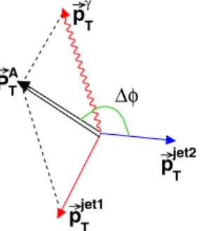
To identify events with two independent parton-parton scatterings that produce aþ3jet final state, we use an angular distribution sensitive to the kinematics of the DP events [24]. We define an azimuthal angle between thepT
vector of theþleading jet system and thepT sum of the two other jets:
SðP~AT; ~PBTÞ; (1)
whereP~AT ¼p~Tþp~jet1T andP~BT ¼p~jet2T þp~jet3T .
Figure 1 shows the sum pT vectors of the þ
leading jet and jet2þjet3 systems in þ3 jet events. In SP events, topologies with two radiated jets emitted close to the leading jet (recoiling against the photon direc-tion in) are preferred and resulting in a peak atS¼. However, this peak is smeared by the effects of additional
γ
T
p
jet1
T
p
jet2
T
p
jet3
T
p
A T
P
B T
P S
∆
FIG. 1 (color online). Diagram showing thepT vectors of the
þleading jet and jet2þjet3systems inþ3jet events.
gluon radiation and detector resolution. For a simple model of DP events, with both the second and third jets originat-ing from the second parton interaction, we have exact pairwise balance inpTin both theþjet and dijet system, and thus theSangle can have any value, i.e., we expect a uniformSdistribution [35].
In this paper, we extend the study of DP interaction to theþ2jet events. In the presence of a DP interaction the second jet in the event originates from a dijet system in the additional parton interaction and the third jet is either not reconstructed or below the pT threshold applied in the
event selection.
In the case ofþ2jet events, we introduce a different angular variable, analogous to (1), to retain sensitivity to DP events. This variable is the azimuthal angle between the
pT vector obtained by pairing the photon and the leading jetpT vectors and the second jetpT vector:
ðP~AT; ~pjet2T Þ: (2)
Figure 2 shows a diagram defining the pT of the two systems inþ2 jet events and the individualpT of the objects. The distribution in þ2 jet events has been used to estimate the DP fraction by the CDF Collaboration [33].
The pT spectrum for jets from dijet events falls faster than that for jets, resulting from ISR and FSR in þjet events, and thus the DP fractions should depend on the jet pT [1,3–6,9,24]. For this reason, the -dependent cross sections and the DP fractions in the þ2 jet events are measured in three pjet2T bins: 15–20, 20–25, and 25–30 GeV. The S-dependent cross section is measured inþ3jet events (a subsample of the inclusive
þ2 jet sample) in a single pjet2T interval, 15–30 GeV. Such a measurement provides good sensitivity to the DP contribution, and discriminating power between different MPI models because the DP fraction inþ3jet events is expected to be higher than that inþ2jet events. This is expected since the second parton interaction will usually produce a dijet final state, while the production of an additional jet in SP events via gluon bremsstrahlung is suppressed by the strong coupling constants.
III. D0 DETECTOR AND DATA SAMPLES
The D0 detector is a general-purpose detector described elsewhere in detail [36]. Here we briefly describe the detector systems most relevant for this analysis. Photon candidates are identified as isolated clusters of energy deposits in the uranium and liquid-argon sampling calo-rimeter. The calorimeter consists of a central section with coverage in pseudorapidityjdetj<1:1[37] and two end calorimeters covering up to jdetj 4:2. The electromag-netic (EM) section of the calorimeter is segmented longi-tudinally into four layers, with transverse segmentation into cells of size detdet ¼0:10:1, except for the third layer, where it is 0:050:05. The hadronic portion of the calorimeter is located behind the EM section. The calorimeter surrounds a tracking system consisting of silicon microstrip and scintillating fiber trackers, both located within a solenoidal magnetic field of approxi-mately 2 T.
The events used in this analysis are required to pass triggers based on the identification of high ET clusters in the EM calorimeter with a shower shape consistent with that expected for photons. These triggers are 100% efficient for photons with transverse momentum pT> 35 GeV. To select photon candidates for our data sample, we use the following criteria [24,38]. EM objects are reconstructed using a simple cone algorithm with a cone size R¼0:2 around a seed tower in space [38].
Regions with poor photon identification capability and limited pT resolution (found at the boundaries between calorimeter modules and between the central and end calorimeters) are excluded from the analysis. Each photon candidate is required to deposit more than 96% of its detected energy in the EM section of the calorimeter and to be isolated in the annular region between
R¼0:2 and R¼0:4 around the center of the cluster:
ðEiso
Tot EisoCoreÞ=EisoCore<0:07, where EisoTot is the total (EMþhadronic) energy in the cone of radius R¼0:4
andEiso
Coreis the EM tower energy within a radiusR¼0:2. The probability for candidate EM clusters to be spatially matched to a reconstructed track is required to be<0:1%, where this probability is calculated using the spatial reso-lutions measured in data. We also require the energy-weighted EM cluster width in the finely-segmented third EM layer to be consistent with that expected for an elec-tromagnetic shower. In addition to calorimeter isolation, we apply track isolation, requiring that the scalar sum of the transverse momenta of tracks in an annulus of0:05
R0:4, calculated around the EM cluster direction, is
less than 1.5 GeV.
Jets are reconstructed by clustering energy deposited in the calorimeter towers using the iterative midpoint cone algorithm [39] with a cone size of 0.7. Jets must satisfy quality criteria that suppress background from lep-tons, pholep-tons, and detector noise effects. To reject back-ground from cosmic rays andW !edecays, the missing
γ T p
jet1
T p
jet2
T p A
T P
φ ∆
transverse momentum, calculated as a vector sum of the transverse energies of all calorimeter cells, is required to be less than 0:7pT. All pairs of objects ði; jÞ in the event (for example, photon and jet or jet and jet) are required to be separated byR¼ ffiffiffiffiffiffiffiffiffiffiffiffiffiffiffiffiffiffiffiffiffiffiffiffiffiffiffiffiffiffiffiffiffiffiffiffiffiffiðijÞ2
þ ðijÞ2 q
>0:9. Each event must contain at least one photon in the pseudorapidity region jdetj<1:0 or 1:5<jdetj<2:5 and at least two (or three) jets with jdetj<3:5. Events are selected with photon transverse momentum50< pT < 90 GeV, leading jet pT>30 GeV, while the next-to-leading (second) jet must have pT >15 GeV. If there is
a third jet with pT >15 GeV that passes the selection
criteria, the event is also considered for the þ3 jet analysis. The higher pT scale (i.e., the scale of the first parton interaction), compared to the lower pT threshold required of the second (and eventual third) jet, results in a good separation between the first and second parton inter-actions of a DP event in momentum space. The recon-structed energy of each jet formed from calorimeter energy depositions does not correspond to the actual energy of the jet particles which enter the calorimeter. It is therefore corrected for the energy response of the calorimeter, en-ergy showering in and out the jet cone, and additional energy from event pileup and multiplepp interactions.
The sample of DP candidates is selected from events with a single reconstructedpp collision vertex. The colli-sion vertex is required to have at least three associated tracks and to be within 60 cm of the center of the detector in the coordinate along the beam (z) axis. The probability for any two pp collisions occurring in the same bunch crossing for which a single vertex is reconstructed was estimated in [24] and found to be<10 3.
IV. SINGLE AND MULTIPLE INTERACTION MODELS
Monte Carlo (MC) samples are used for two purposes in this analysis. First, we use them to calculate reconstruction efficiencies and to unfold the data spectra to the particle level. Secondly, differential cross sections of þjet events simulated using different MPI models as imple-mented in the PYTHIA and SHERPA [40] event generators are compared with the measured cross sections.
There are two main categories of MPI models based on different sets of data used in the determination of the models parameters (it is customary to refer to different models and to their settings as ‘‘tunes’’). The two catego-ries, ‘‘old’’ and ‘‘new,’’ correspond to different approaches in the treatment of MPI, ISR, and FSR, and other effects [10,12]. The main difference between the new [11] and the old models is the implementation of the interplay between MPI and ISR, i.e., considering these two effects in parallel, in a common sequence of decreasing pT values. In the old models, ISR and FSR were included only for the hardest interaction, and this was done before any additional
interactions were considered. In the new models, all parton interactions include ISR and FSR separately for each in-teraction. The new models, especially those corresponding to the Perugia family of tunes [10], also allow for a much wider set of physics processes to occur in the additional interactions. A detailed description of the differentPYTHIA MPI models can be found elsewhere [10,11]. Here we provide a brief description of the models considered in our analysis. They include Perugia-0 (P0, the default model in the Perugia family [10]); P-hard and P-soft, which explore the dependence on the strength of ISR/FSR effects, while maintaining a roughly-consistent MPI model as implemented in the P0 tune; P-nocr, which excludes any color reconnections in the final state; and P-X and P-6, which are P0 modifications based on the MRST LO* and CTEQ6L1 PDF sets, respectively (P0 uses CTEQ5L as a default). We also compare data with predictions deter-mined using tunes A and DW as representative of the old MPI models.
The measured cross sections are also compared with predictions obtained from the SHERPA event generator, which also contains a simulation of MPI. Its initial mod-elling was similar to tune A from PYTHIA [7], but it has evolved and now is characterized, in particular, by (a) showering effects in the second interaction and (b) a combination of the Catani-Krauss-Kuhn-Webber (CKKW) merging approach with the MPI modeling [40,41]. Another distinctive feature ofSHERPAis the modeling of the parton-to-photon fragmentation contributions through the incor-poration of QED effects into the parton shower [42].
The data are also compared with models without MPI, in which the photon and all the jets are produced exclusively in SP scattering. Such events are simulated in bothPYTHIA and SHERPA. In PYTHIA, only 2!2 diagrams are simu-lated, resulting in the production of a photon and a leading jet. With the MPI event generation switched off, all the additional (to the leading) jets are produced in the parton shower development in the initial and final states. We refer to such SP events as ‘‘PYTHIASP’’ events. InSHERPA, up to two extra partons (and thus jets) are allowed at the matrix element level in the 2! f2;3;4g scattering, but jets can also be produced in parton showers. To provide a matching between the matrix-element partons and parton shower jets, we follow the recommendation provided in [42] and choose the following ‘‘matching’’ parameters: the energy scale Q0 ¼30 GeV and the spatial scaleD¼0:4, where
D is taken to be of the size of the photon isolation cone [43]. This is the default scheme for the production ofþ
SHERPASP events in which all of the extra jets are produced (as in PYTHIA) in the parton shower with only a 2!2
matrix element, and call this set ‘‘SHERPA-4SP.’’
V. DATA ANALYSIS AND CORRECTIONS
A. Background studies
The main background to isolated photons comes from jets in which a large fraction of the transverse momentum is carried by photons from 0, , or K0
s decays. The
photon-enhancing criteria described in Sec.IIIare devel-oped to suppress this background. The normalizedSand
distributions are not very sensitive to the exact amount of background from events with misidentified photons. To estimate the photon fractions in thebins, we use the output of two neural networks (NN) [38]. These NNs are constructed using theJETNETpackage [44] and are trained to discriminate between photon and EM-jets in the central and end calorimeter regions using calorimeter shower shape and track isolation variables [38]. The distribution of the photon NN output for the simulated photon signal and for the dijet background samples are fitted to data in eachbin using a maximum likelihood fit [45] to obtain the fractions of signal events in the data. To obtain a more statistically significant estimate of the photon purity in the
bins, we use a singlepjet2T bin:15< pjet2T <30 GeV. The fit results show that theþjet signal fractions in all
bins agree well with a constant value,0:690:03in the central and0:710:02in the end calorimeter regions. The sensitivity of theSand distributions to this background from jets is also examined by considering two data samples in addition to the sample with the default photon selections: one with relaxed and another with tighter track and calorimeter isolation requirements. According to MC estimates, in those two samples the fraction of background events should either increase or decrease by (30–35)% with respect to the default sample. We study the variation of theSandnormalized cross sections in data by comparing the relaxed and tighter data sets with the default set. We find that the cross section variations are within 5%.
B. Efficiency and unfolding corrections
To selectþ2jet andþ3jet events, we apply the selection criteria described in Sec.III. The selected events are then corrected for selection efficiency, acceptance, and event migration effects in bins of S and . These corrections are calculated using MC events generated us-ing PYTHIA with tune P0, as discussed in Sec. IV. The generated MC events are processed through aGEANT-based [46] simulation of the D0 detector response. These MC events are then processed using the same reconstruction code as used for the data. We also apply additional smearing to the reconstructed photon and jet pT so that
the resolutions in MC match those observed in data.
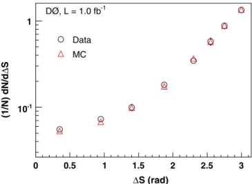
The reconstructed Sand distributions in the simu-lated events using the P0 tune are found to describe the data. In addition to the simulation with the default tune P0, we have also considered P0 MC events that have been reweighted to reproduce the pT distributions in data. After such reweighting, the reconstructed S and
distributions give an excellent description of the data. Figs. 3 and 4 show the normalized distributions as a function ofSforþ3jet andforþ2jet events (for thepjet2T bin 15–20 GeV, chosen as an example) in data and in the reweighted MC.
Three sets of corrections are applied in data to obtain the differential cross sections which we then compare with the various MPI models. We apply them to correct for detector and reconstruction inefficiencies and for bin migration effects. The first correction deals with the possibility that, due to the detector and reconstruction effects, our selected event sample may contain events which would fail the selection criteria at the particle level. The data distributions are corrected, on a bin-by-bin basis, for the fraction of events of this type. We also apply a correction for events which fail the selection requirement at the reconstruction level. Systematic uncertainties are assigned on these two correction factors to account for uncertainties on the pho-ton and jet identification, the jet energy scale (JES) and resolution, and vary in theS() bins up to 12% (18%) in total. They are dominated by the JES uncertainties. The overall corrections obtained with the default P0 and with the reweighted MC samples agree within about 5% for most Sand bins and differ by at most 25%. Since we are measuring normalized cross sections, the absolute values of the corrections are not important, and we need only their relative dependence onSand.
The third correction accounts for the migration of events between different bins of the S and distributions,
S (rad) ∆
0 0.5 1 1.5 2 2.5 3
S
∆
(1/N) dN/d
-1
10 1
Data
MC
-1
DØ, L = 1.0 fb
which is caused by the finite photon and jet angular reso-lutions and by energy resolution effects, and can change thepT ordering of jets between the reconstruction and the
particle level. To obtain theSanddistributions at the particle level, we follow the unfolding procedure described in the Appendix, based on the Tikhonov regularization method [47–50]. The bin sizes for theSand distri-butions are chosen to have sensitivity to different MPI models (which is largest for small S and angles) while keeping good statistics and the bin-to-bin migration small. The statistical uncertainties (stat) are in the range (10–18)%. They are due to the procedure of regularized unfolding and take into account the correlations between the bins. The correlation factor for adjacent bins in the unfolded distributions is about (30–45)%, and it is reduced to10%for other (next-to-adjacent) bins. To validate the unfolding procedure, a MC closure test is performed. We compare the unfolded MC distribution to the true MC distribution and find that they agree within statistical uncertainties.
VI. DIFFERENTIAL CROSS SECTIONS AND COMPARISON WITH MODELS
In this section, we present the four measurements of normalized differential cross sections, ð1=3jÞd3j= dSin a singlepjet2T bin (15–30 GeV) forþ3jet events andð1=2jÞd2j=din threepjet2T bins (15–20, 20–25,
and 25–30 GeV) for þ2 jet events. The results are presented numerically in Tables I, II, III, and IV as a function of S and , with the bin centers estimated using the theoretical predictions obtained using the P0 tune. The column ‘‘Ndata’’ shows the number of selected data events in eachS() bin at the reconstruction level. The differential distributions decrease by about 2 orders
of magnitude when moving from the S () bin
2.85–3.14 radians to the bin 0.0–0.7 radians and have a total uncertainty (tot) between 7% and 30%. Here tot is defined as a sum in quadrature of statistical (stat) and systematical (syst) uncertainties. It is dominated by sys-tematic uncertainties. The sources of syssys-tematic uncertain-ties are the JES (2–17%), largest at the small angles, unfolding (5–18%), jet energy resolution simulation in MC events (1–7%), and background contribution (up to 5%).
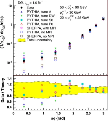
The results are compared in Figs. 4–7 to predictions from different MPI models implemented in PYTHIA and SHERPA, as discussed in Sec.IV. We also show predictions of SP models inPYTHIAandSHERPA(SHERPA-1model). In the QCD NLO predictions, only final states with aþ2
jet topology are considered, and thus for the direct photon production diagrams, we should have ¼. The
angle may differ fromdue to photon production through a parton-to-photon fragmentation mechanism. Even if we take into account this production mechanism, which is included in the JETPHOX [51] NLO QCD calculations, only the two highest bins receive significant contributions.
Figures 4–7 show the sensitivity of the two angular variables S and to the various MPI models, with predictions varying significantly and differing from each (rad)
φ ∆
0 0.5 1 1.5 2 2.5 3
φ
∆
(1/N) dN/d
-1 10
1
Data MC
-1
DØ, L = 1.0 fb
FIG. 4 (color online). Normalizeddistribution for data and for the reweighted MC sample in the range 15< pjet2T < 20 GeV.
TABLE I. Measured normalized differential cross sections ð1=3jÞd3j=dS for 15<
pjet2T <30 GeV.
Sbin (rad) hSi(rad) Ndata Normalized cross section Uncertainties (%)
stat syst tot
0.00–0.70 0.36 495 2:9710 2 11.3 14.7 18.6
0.70–1.20 0.97 505 4:7410 2 12.3 15.6 19.9
1.20–1.60 1.42 498 5:8010 2 13.4 15.8 20.7
1.60–2.15 1.90 1315 1:1110 1 7.5 15.3 17.0
2.15–2.45 2.32 1651 2:3810 1 6.0 12.0 13.4
2.45–2.65 2.56 1890 4:0410 1 5.6 13.6 14.7
2.65–2.85 2.76 3995 8:5910 1 3.2 5.6 6.4
other by up to a factor 2.5 at small S and , in the region where the relative DP contribution is expected to be the highest. The sensitivity is reduced by the choice of SP model, for which we derive an upper value of 25% com-paring the ratios of predictions from various models (PYTHIA,SHERPA-2,-3, -4). This upper value is considerably smaller than the difference between the various MPI models.
Tables Vand VI are complementary to Figs. 4–7 and show the2=ndfvalues of the agreement between theory
and data for each model. Herendfstands for the number of degrees of freedom (taken as the number of bins, Nbins
minus 1), and2 is calculated as
2
¼ X
Nbins
i¼1
ðDi TiÞ2
2
i;unc
; (3)
whereDiandTirepresent the cross section values in theith
bin of data and a theoretical model, respectively, while
2
i;unc is the total uncorrelated uncertainty in this bin. The
TABLE II. Measured normalized differential cross sections ð1=2jÞd2j=d for 15<
pjet2T <20 GeV.
bin (rad) hi(rad) Ndata Normalized cross section Uncertainties (%)
stat syst tot
0.00–0.70 0.36 1028 2:4910 2 9.4 19.1 21.3
0.70–1.20 0.96 822 3:0610 2 11.8 20.3 23.4
1.20–1.60 1.42 1149 5:6810 2 9.6 15.5 18.2
1.60–2.15 1.92 3402 1:2910 1 4.9 11.5 12.5
2.15–2.45 2.32 4187 3:0610 1 4.5 9.5 10.5
2.45–2.65 2.56 5239 5:8810 1 4.0 6.3 7.4
2.65–2.85 2.76 8246 9:4310 1 3.0 6.8 7.5
2.85–3.14 3.01 20 337 1:63100 1.1 12.3 12.3
TABLE III. Measured normalized differential cross section ð1=2jÞd2j=d for 20<
pjet2T <25 GeV.
bin (rad) hi(rad) Ndata Normalized cross section Uncertainties (%)
stat syst tot
0.00–0.70 0.35 388 1:1710 2 12.5 23.2 26.4
0.70–1.20 0.96 358 1:7510 2 17.7 22.2 28.5
1.20–1.60 1.42 489 3:2910 2 15.6 17.0 23.1
1.60–2.15 1.92 1848 9:8410 2 6.2 13.8 15.1
2.15–2.45 2.33 2682 2:8010 1 4.6 8.2 9.4
2.45–2.65 2.56 3208 5:2110 1 4.5 7.1 8.4
2.65–2.85 2.77 5404 9:0110 1 3.2 7.3 8.0
2.85–3.14 3.02 15 901 1:88100 1.0 10.8 10.8
TABLE IV. Measured normalized differential cross section ð1=2jÞd2j=d for 25<
pjet2T <30 GeV.
bin (rad) hi(rad) Ndata Normalized cross section Uncertainties (%)
stat syst tot
0.00–0.70 0.32 158 6:8210 3 16.1 19.8 25.5
0.70–1.20 0.94 155 1:1110 2 20.9 16.4 26.6
1.20–1.60 1.45 190 1:8710 2 24.0 17.9 30.0
1.60–2.15 1.92 910 7:0010 2 7.0 15.9 17.4
2.15–2.45 2.32 1683 2:5010 1 5.0 8.6 9.9
2.45–2.65 2.57 2155 4:9310 1 4.5 8.9 10.0
2.65–2.85 2.77 3894 9:0910 1 3.1 7.5 8.1
latter is composed of the uncertainties for the corrections in the unfolding procedure (Sec. V B), the statistical uncer-tainties of the datastatand the theoretical model, respec-tively. The uncorrelated uncertainty2
i;uncis always larger than all remaining correlated systematic uncertainties.
Since small angles (SðÞ&2) are the most sensitive to DP contributions, we calculate the 2=ndfseparately for these bins. From Figs. 4–7and Tables Vand VI, we conclude the following: (a) the predictions derived from SP models do not describe the measurements; (b) the data
TABLE VI. The results of a2test of the agreement between data points and theory predictions for theS(þ3jet) and the
(þ2jet) distributions forSðÞ 2:15 rad. Values are2=ndf.
Variable pjet2T (GeV) SP model MPI model
PYTHIA SHERPA A DW S0 P0 P-nocr P-soft P-hard P-6 P-X SHERPA
S 15–30 10.9 11.3 31.0 42.9 3.4 0.4 0.5 4.9 0.9 0.5 0.4 2.6
15–20 30.2 26.0 40.7 61.1 2.2 0.9 1.6 1.5 1.2 1.2 1.0 2.4
20–25 15.4 12.1 6.8 18.0 1.0 1.8 2.7 1.7 1.5 2.5 2.4 0.6
25–30 7.1 5.3 1.3 5.6 1.6 1.1 1.0 2.1 0.3 1.4 1.6 0.5
TABLE V. The results of a2test of the agreement between data points and theory predictions for theS(þ3jet) and(þ2
jet) distributions for0:0SðÞ rad. Values are2=ndf.
Variable pjet2T (GeV) SP model MPI model
PYTHIA SHERPA A DW S0 P0 P-nocr P-soft P-hard P-6 P-X SHERPA
S 15–30 7.7 6.0 15.6 21.4 2.2 0.4 0.5 2.9 0.5 0.4 0.5 1.9
15–20 16.6 11.7 19.6 27.7 1.6 0.5 0.9 1.6 0.9 0.6 0.8 1.2
20–25 10.2 5.9 4.0 7.9 1.1 0.9 1.4 2.1 1.1 1.3 1.5 0.4
25–30 7.2 3.5 2.8 3.0 2.4 1.1 1.1 3.7 0.2 1.3 1.9 0.7
S
∆
/d
3j
γ
σ
) d
3j
γ
σ
(1/
-1 10
1
-1 = 1.0 fb int DØ, L
Data
PYTHIA, tune A PYTHIA, tune DW PYTHIA, tune S0 PYTHIA, tune P0 SHERPA, with MPI PYTHIA, no MPI SHERPA, no MPI Total uncertainty
< 90 GeV
γ
T 50 < p
> 30 GeV jet1
T p
< 30 GeV jet2
T 15 < p
> 15 GeV jet3
T p
S (rad) ∆
0 0.5 1 1.5 2 2.5 3
Data / Theory
0.4 0.6 0.8 1 1.2 1.4
S (rad) ∆
0 0.5 1 1.5 2 2.5 3
Data / Theory
0.4 0.6 0.8 1 1.2 1.4
FIG. 5 (color online). Normalized differential cross section in þ3jet events,ð1=3jÞd3j=dS, in data compared to MC models and the ratio of data over theory, only for models including MPI, in the range15< pjet2T <30 GeV.
φ
∆
/d
2j
γ
σ
) d
2j
γ
σ
(1/
-2 10
-1 10
1 10
-1
= 1.0 fb
int
DØ, L
Data
PYTHIA, tune A PYTHIA, tune DW PYTHIA, tune S0 PYTHIA, tune P0 SHERPA, with MPI PYTHIA, no MPI SHERPA, no MPI Total uncertainty
< 90 GeV
γ
T 50 < p
> 30 GeV jet1
T p
< 20 GeV jet2
T 15 < p
(rad) φ ∆
0 0.5 1 1.5 2 2.5 3
Data / Theory
0.4 0.6 0.8 1 1.2 1.4
(rad) φ ∆
0 0.5 1 1.5 2 2.5 3
Data / Theory
0.4 0.6 0.8 1 1.2 1.4
FIG. 6 (color online). Normalized differential cross section in þ2jet events,ð1=2jÞd2j=d, in data compared to MC models and the ratio of data over theory, only for models including MPI, in the range15< pjet2T <30 GeV.
favor the predictions of the newPYTHIAMPI models (P0, P-hard, P-6, P-X, P-nocr) and to a lesser extent S0 and SHERPAwith MPI; and (c) the predictions from tune A and DW MPI models are disfavored.
VII. FRACTIONS OF DOUBLE PARTON EVENTS IN THEþ2JET FINAL STATE
The comparison of the measured cross section with models (Sec.VI) shows clear evidence for DP scattering. We use the measurement of the differential cross section with respect toand predictions for the SP contributions to this cross sections in different models to determine the fraction of þ2 jet events which originate from DP interactions as a function of the second parton interaction scale (pjet2T ) and of. Because of ISR and FSR effects the
pT balance vectors of each system may be nonzero and have an arbitrary orientation with respect to each other [35], which leads to a uniform distribution for DP events.
Using the uniform distribution as the DP model template and theSHERPA-1prediction as the SP model template, we can fit thedistributions measured in data and obtain the fraction of DP events from a maximum likelihood fit [45]. We repeat this procedure in three independent ranges of
pjet2T . The distributions in data, SP, and DP models, as well as a sum of the SP and DP distributions, weighted with
their respective fractions, are shown in Figs.8–10for the threepjet2T intervals. The sum of the SP and DP predictions reproduces the data well. The measured DP fractions (fdp2j) are presented in TableVII.
The uncertainties in the DP fractions are due to the fit, the total (statistical plus systematic) uncertainties on the data points, and the choice of SP model. The effect from the second source is estimated by varying all the data points simultaneously up and down by the total experimen-tal uncertainty (tot). The uncertainties due to the SP model are estimated by considering SP models (Sec.IV) that are different from the default choice of SHERPA-1: -2, -3, -4, as well asPYTHIASP predictions. The measured DP fractions with all sources of uncertainties in each pjet2T bin are summarized in Table VII. The DP fractions in þ2jet events, fdp2j, decrease as a function of pjet2T from ð11:61:0Þ% in the bin 15–20 GeV, to ð5:01:2Þ% in the bin 20–25 GeV, and ð2:20:8Þ% in the bin 25–30 GeV. The estimated DP fraction inþ2jet events selected with pT>16 GeV and pjetT >8 GeV from the CDF Collaboration [33] is14þ87%, which is in qualitative agreement with an extrapolation of our measured DP frac-tions to lower jetpT.
The DP fractions shown in TableVIIare integrated over the entire region0. However, from Figs.8–10,
φ ∆ /d 2j γ σ ) d 2j γ σ (1/ -2 10 -1 10 1 10 -1 = 1.0 fb int DØ, L
Data
PYTHIA, tune A PYTHIA, tune DW PYTHIA, tune S0 PYTHIA, tune P0 SHERPA, with MPI PYTHIA, no MPI SHERPA, no MPI Total uncertainty
< 90 GeV
γ
T 50 < p
> 30 GeV jet1
T p
< 25 GeV jet2
T 20 < p
(rad) φ ∆
0 0.5 1 1.5 2 2.5 3
Data / Theory
0.4 0.6 0.8 1 1.2 1.4 (rad) φ ∆
0 0.5 1 1.5 2 2.5 3
Data / Theory
0.4 0.6 0.8 1 1.2 1.4
FIG. 7 (color online). Normalized differential cross section in þ2jet events,ð1=2jÞd2j=d, in data compared to MC models and the ratio of data over theory, only for models including MPI, in the range20< pjet2T <25 GeV.
φ ∆ /d 2j γ σ ) d 2j γ σ (1/ -2 10 -1 10 1 10 -1 = 1.0 fb int DØ, L
Data
PYTHIA, tune A PYTHIA, tune DW PYTHIA, tune S0 PYTHIA, tune P0 SHERPA, with MPI PYTHIA, no MPI SHERPA, no MPI Total uncertainty
< 90 GeV
γ
T 50 < p
> 30 GeV jet1
T p
< 30 GeV jet2
T 25 < p
(rad) φ ∆
0 0.5 1 1.5 2 2.5 3
0.4 0.6 0.8 1 1.2 1.4 1.6 (rad) φ ∆
0 0.5 1 1.5 2 2.5 3
Data / Theory
0.4 0.6 0.8 1 1.2 1.4 1.6
the fraction of DP events is expected to be higher at smaller
. To determine the fractions as a function of, we perform a fit in the differentregions by excluding the bins at high ; specifically, by considering the
regions 0–2.85, 0–2.65, 0–2.45, 0–2.15, and 0–1.60. The DP fractions for theseregions are shown in TableVIII for the three pjet2T intervals. The DP fractions with total uncertainties as functions of the upper limit on
(max) for all the p jet2
T bins are also shown in Fig. 11.
As expected, they grow significantly towards the smaller angles and are higher for smallerpjet2T bins.
VIII. FRACTIONS OF TRIPLE PARTON EVENTS IN THEþ3JET FINAL STATE
In this section, we estimate the fraction of þ3 jet events from triple parton interactions (TP) in data as a function of pjet2T . In þ3 jet TP events, the three jets come from three different parton interactions, one þ
jet and two dijet final states. In each of the two dijet events, one of the jets is either not reconstructed or below the 15 GeVpT selection threshold.
In our previous study of DP þ3 jet events [24], we built a data-driven model of inclusive DP interactions (MixDP) by combining þjet and dijet events from data, and obtaining the þ3jetþX final state. However, since each component of the MixDP model may contain two (or more) jets, where one jet is due to an additional parton interaction, the model simulates the properties of ‘‘double plus triple’’ parton interactions. Therefore, the ‘‘DP’’ fractions found earlier in the þ3
jet data (shown in Table III of [24]) take into account a contribution from TP interactions as well. These fractions are also shown in the second column of TableIX. Thus, if we calculate the fractions of TP events in the MixDP sample, defined asftpdpþtp, we can calculate the TP fractions in theþ3jet data,ftp3j, as
(rad) φ ∆
0 0.5 1 1.5 2 2.5 3
φ
∆
/d
2j
γ
σ
) d
2j
γ
σ
(1/
-2
10
-1
10
1 Data
DP model SP model
)
2j
γ
dp
+ SP(1-f
2j
γ
dp
DP f
-1
DØ, L = 1.0 fb jet2 < 20 GeV
T
15 < p
1.0% ± = 11.6
2j
γ
dp
f
FIG. 9 (color online). distribution in data, SP, and DP models, and the sum of the SP and DP contributions weighted with their fractions for15< pjet2T <20 GeV.
(rad) φ ∆
0 0.5 1 1.5 2 2.5 3
φ
∆
/d
2j
γ
σ
) d
2j
γ
σ
(1/
-2
10
-1
10
1 Data
DP model
SP model )
2j
γ
dp
+ SP(1-f
2j
γ
dp
DP f
-1
DØ, L = 1.0 fb jet2 < 25 GeV
T
20 < p
1.2% ± = 5.0
2j
γ
dp
f
FIG. 10 (color online). Same as in Fig.9, but for25< pjet2T < 25 GeV.
TABLE VII. Fractions of DP events (%) with total uncertain-ties for0in the threepjet2T bins.
pjet2T (GeV) hpjet2T i(GeV) fdp2j(%) Uncertainties (in %)
Fit tot SP model
15–20 17.6 11:61:4 5.2 8.3 6.7 20–25 22.3 5:01:2 4.0 20.3 11.0 25–30 27.3 2:20:8 27.8 21.0 17.9
TABLE VIII. DP fractions (%) in data as a function of theinterval for threepjet2T bins.
pjet2T (GeV) interval (rad)
0– 0–2.85 0–2.65 0–2.45 0–2.15 0–1.6
15–20 11:61:4 18:22:4 25:02:9 33:73:8 45:05:5 47:411:4 20–25 5:01:2 9:41:2 13:42:1 19:63:1 28:14:3 63:717:2 25–30 2:20:8 3:81:3 5:01:5 6:22:2 9:84:5 27:811:5
ftp3j¼f dpþtp
tp f
3j
dpþtp; (4)
wherefdp3þjtpis the fraction ofDPþTPevents in theþ3
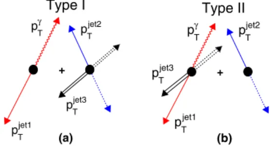
jet sample. Figure12shows two possible ways in which a DP event and an SP event can be combined to form aþ3
jet event which is a part of the MixDP sample, with details on the origin of the various parts of the event given in the caption. Contributions from other possible MixDP configu-rations are negligible (&1%). In [24], we calculated how often each component, Type I and II, is found in the model. TableIXshows that the events of Type II are dominant in all bins.
Thus, the fraction of TP configurations (Fig.12) in the MixDP model,fdptpþtp, can be calculated as
fdptpþtp¼FType IIf 2j
dp þFType Ifdpjj; (5)
where fdp2j and fjjdp are the fractions of events with DP scattering resulting inþ2jet and dijet final states. We separately analyze each of the event types of Fig.12. The fraction of events having a second parton interaction with a dijet final state with cross sectionjjcan be defined using
the effective cross sectioneff asfdpjj ¼jj=ð2effÞ. The cross section for a DP scattering producing two dijet final states can be presented then asjj;jjdp ¼jjfjj
dp [7,9]. The
fractionfdpjj is estimated using dijet events simulated with PYTHIA. We calculate the jet cross sectionsjjfor
produc-ing at least one jet in the three pT bins with jjet j<3:5. The effective cross sectioneffis taken as an average of the CDF [21] and D0 [24] measurements,averageeff ¼15:5 mb. The determined fractions are shown in the third column of Table X. We assume that the estimates, done at the particle level, are also approximately correct at the recon-struction level. We take an uncertainty on these numbers
fdpjj ¼fjjdp.
The fractions of theþ2jet events in which the second jet is due to an additional parton scattering are estimated in the previous section and are much higher than fdpjj. However, since we estimate the TP fraction in data at the reconstruction level, we repeat the same fitting procedure used for the extraction offdp2jfrom thedistributions in the reconstructed data and SP þ2 jet MC events. The results of the fit in the threepjet2T intervals are summarized in the second column of TableX. Here the total uncertain-tiestotare due to the statistical and systematic uncertain-ties shown in Tables II, III, and IV, but excluding the uncertainties from the unfolding.
(rad) φ ∆
0 0.5 1 1.5 2 2.5 3
φ
∆
/d
2j
γ
σ
) d
2j
γ
σ
(1/
-2
10
-1
10
1 Data
DP model SP model
)
2j
γ
dp
+ SP(1-f
2j
γ
dp
DP f
-1
DØ, L = 1.0 fb jet2 < 30 GeV
T
25 < p
0.8% ± = 2.2
2j
γ
dp
f
FIG. 11 (color online). Same as in Fig.9, but for25< pjet2T < 30 GeV.
(rad)
max
φ ∆
1.6 1.8 2 2.2 2.4 2.6 2.8 3
Fraction of DP events
0.1 0.2 0.3 0.4 0.5 0.6 0.7 0.8 0.9
< 20 GeV
jet2 T
15 < p
< 25 GeV
jet2 T
20 < p
< 30 GeV
jet2 T
25 < p
-1
DØ, L = 1.0 fb
+ 2 jet events γ
FIG. 12 (color online). Fractions of DP events with total un-certainties inþ2jet final state as a function of the upper limit onfor the threepjet2T intervals.
TABLE IX. Fractions ofDPþTPevents with total uncertain-ties inþ3jet data (fdp3þjtp) and fractions of Type I (II) events in the data-driven DP model (FType IðIIÞ) in the threep
jet2
T bins.
pjet2T (GeV) fdp3þjtp(%) FType I FType II
15–20 46:64:1 0.26 0.73
20–25 33:42:3 0.22 0.78
25–30 23:52:7 0.14 0.86
TABLE X. Fractions of DP events inþ2jet (fdp2j) and dijet (fjjdp) final states as well the fraction of TP configurations in the MixDP model (fdptpþtp) in the threep
jet2
T bins.
pjet2T (GeV) fdp2j(%) fjjdp(%) ftpdpþtp(%)
By substitutingfdpjj and fdp2jinto Eq. (5), we calculate the TP fractions ftpdpþtp in the MixDP model. They are shown in the last column of Table X. The TP fraction in the similar data-driven MixDP model in the CDF analysis [21] for (JES uncorrected) 5< pjet2T <7 GeV was esti-mated as 17þ4
8%, i.e., a value that is higher, on average,
than our TP fractions measured at higher jet pT, but in agreement with an extrapolation of our observed trend to lower jetpT.
By substitutingfdptpþtpand theDPþTPfractions inþ
3 jet data fdp3þjtp from [24] into Eq. (4), we get the TP fractions in theþ3jet data,ftp3j, which are shown in the second column of Table XI. They are also presented in Fig.13. The pure DP fractions,fdp3j, can then be obtained by subtracting the TP fractions ftp3j from the inclusive
DPþTPfractionsfdp3þjtp.
The last column of TableXIshows the ratios of the TP to DP fractions ftp3j=fdp3j in þ3 jet events. Since the probability of producing each additional parton scattering with a dijet final state is expected to be directly propor-tional tojj=
eff, thef 3j
tp =f 3j
dp ratio should be approxi-mately proportional to the jet cross sectionjj, and drop
correspondingly as a function of the jet pT. This trend is confirmed in TableXI.
IX. SUMMARY
We have studied the azimuthal correlations inþ3jet and þ2 jet events and measured the normalized differential cross sections ð1=3jÞd3j=dS and
ð1=2jÞd2j=d in three bins of the second jet pT.
The results are compared to different MPI models and demonstrate that the predictions of the SP models do not describe the measurements and an additional contribution from DP events is required to describe the data. The data favor the predictions of the newPYTHIAMPI models with
pT-ordered showers, implemented in the Perugia and S0 tunes, and alsoSHERPAwith its default MPI model, while predictions from previousPYTHIAMPI models, with tunes A and DW, are disfavored.
We have also estimated the fractions of DP events in the
þ2jet samples and found that they decrease in the bins ofpjet2T asð11:61:0Þ%for 15–20 GeV,ð5:01:2Þ%for 20–25 GeV, andð2:20:8Þ%for 25–30 GeV. Finally, for the first time, we have estimated the fractions of TP events in theþ3jet data. They vary in thepjet2T bins asð5:5 1:1Þ% for 15–20 GeV,ð2:10:6Þ% for 20–25 GeV, and ð0:90:3Þ%for 25–30 GeV.
The measurements presented in this paper can be used to improve the MPI models and reduce the existing theoreti-cal ambiguities. This is especially important for studies in which a dependence on MPI models is a significant uncer-tainty (such as the top quark mass measurement), and in searches for rare processes, for which DP events can be a sizable background.
ACKNOWLEDGMENTS
We thank the staffs at Fermilab and collaborating insti-tutions, and acknowledge support from the DOE and NSF
TABLE XI. Fractions of TP events (%) and the ratio of TP/DP fractions in the threepjet2T bins ofþ3jet events.
pjet2T (GeV) ftp3j(%) f 3j
tp =f 3j
dp
15–20 5:51:1 0:1350:028
20–25 2:10:6 0:0660:020
25–30 0:90:3 0:0380:014
+ Type I
(a) γ
T
p
jet1 T
p
jet2 T
p
jet3 T
p
+ Type II
(b)
γ
T p
jet1 T p
jet2 T p
jet3 T p
FIG. 13 (color online). Two possible combinations of events present in the MixDP sample that actually represent the contri-bution from triple scattering events in theþ3jet final state: (a) a þ1 jet event mixed with a double-dijet DP event, where one jet of each dijet is lost or not reconstructed (Type I); (b) a DP event in theðþ1jetÞ þdijet final state with one jet from the dijet lost, mixed with a dijet event with one jet lost (Type II). Dashed lines correspond to the lost jets.Fractions of TP events with total uncertainties in þ3 jet final state as a function ofpjet2T .
(GeV)
jet2 T
p
16 18 20 22 24 26 28 30
Fraction of TP events
0.01 0.02 0.03 0.04 0.05 0.06 0.07 0.08
-1
DØ, L = 1.0 fb γ + 3 jet events
FIG. 14 (color online). Fractions of TP events with total un-certainties inþ3jet final state as a function ofpjet2T .
(USA); CEA and CNRS/IN2P3 (France); FASI, Rosatom, and RFBR (Russia); CNPq, FAPERJ, FAPESP, and
FUNDUNESP (Brazil); DAE and DST (India);
Colciencias (Colombia); CONACyT (Mexico); KRF and KOSEF (Korea); CONICET and UBACyT (Argentina); FOM (the Netherlands); STFC and the Royal Society (United Kingdom); MSMT and GACR (Czech Republic); CRC Program and NSERC (Canada); BMBF and DFG (Germany); SFI (Ireland); the Swedish Research Council (Sweden); and CAS and CNSF (China).
APPENDIX
In this appendix we discuss the unfolding procedure used to correct the measuredSanddistributions to the particle level in order to obtain a nonparametric esti-mate of the trueSand distributions from the mea-sured (reconstructed) distribution, taking into account possible biases and statistical uncertainties. We use the following approach to extract the desired distributions from our measurements. The observed distribution is the result of the convolution of a resolution function with the desired distribution at the particle level. After the discreti-zation inS=bins, the resolution function is a smear-ing matrix, and distributions on both particle level and reconstruction level become discrete distributions (i.e., histograms). The smearing matrix is stochastic: all ele-ments are non-negative and the sum of eleele-ments in each column is equal to 1. Thus, the matrix columns are the probability density functions that relate each bin in a histogram at the particle level to the bins in a histogram at the reconstruction level. We split the fullS() range ½0; into eight bins and fix two bins at smallS() angles as 0–0.7 and 0.7–1.2 radians. These two bins are the most sensitive to a contribution from DP scattering, and their widths are chosen as a compromise between sensi-tivity to DP events and the size of the relative statistical uncertainty. The sizes of the other six bins are varied to minimize the ratio of maximum and minimum eigenvalues of the smearing matrix, defined as the condition number. This ratio, greater than unity, represents the scaling factor for the statistical uncertainties arising from the transfor-mation of the differential cross sections from the recon-structed to the particle level. The same binning is used for the reconstructed and particle level distributions. We build the smearing matrix using reconstructed and particle level events in the reweighted MC sample, described in
Sec.V B. To decrease the statistical uncertainties (stat), we use a Tikhonov regularization procedure [47–50] for the matrix. This unfolding procedure may introduce a bias (b). We optimize the regularization by finding a balance be-tweenstat andbaccording to the following criterion: we minimize the following function ofstat andbin the first two bins, 0–0.7 and 0.7–1.2:
U¼ ½ð0:5b1Þ2þ ðstat;1Þ2 þ ½ð0:5b2Þ2þ ðstat;2Þ2: (6)
These two bins, being the most sensitive to contributions from DP scatterings, are the most important for our analy-sis. We perform the regularization of the smearing matrix by adding a non-negative parameter to all diagonal elements of the smearing matrix. The matrix columns are then renormalized to make the matrix stochastic again (¼0 is equivalent no regularization, while for! 1
the smearing matrix becomes the identity matrix). The smallest uncertainties U are usually achieved with
¼0:3–0:5. An estimate of the unfolded distribution is obtained by multiplying the histogram (vector) of the measured Sanddistributions by the inverted regu-larized smearing matrix. We use the sample of the re-weighted MC events to get an estimate of the statistical uncertainties and the bias in bins of the unfolded distribu-tion. To accomplish this, we choose a MC subsample with the number of events equal to that of the selected data sample and having a discrete distribution (histogram) at the reconstruction level that is almost identical to that in data. We randomize the MC histogram at the reconstruction level repeatedly (100 000 times) according to a multino-mial distribution and multiply this histogram by the in-verted regularized smearing matrix for each perturbation. We obtain a set of unfolded distributions at the particle level. Using this set and the true distribution for this MC sample, we estimate the statistical uncertaintystatand the biasbas the root-mean-square (RMS) and the mean of the distribution ‘‘(true-unfolded)/true’’ for eachS() bin. The unfolded distribution is then corrected for the bias in each bin. We assign half of the bias as a systematic uncer-tainty on this correction. The overall unfolding corrections vary up to 60%, being largest at the small angles. The total uncertainties, estimated in each bin ifor theSand
distributions as ffiffiffiffiffiffiffiffiffiffiffiffiffiffiffiffiffiffiffiffiffiffiffiffiffiffiffiffiffiffiffiffiffiffiffiffiffiffið0:5biÞ2þ ð stat;iÞ2
q
, vary between 10% and 18%.
[1] P. V. Landshoff and J. C. Polkinghorne,Phys. Rev. D18, 3344 (1978).
[2] C. Goebel, F. Halzen, and D. M. Scott,Phys. Rev. D22, 2789 (1980).
[3] F. Takagi,Phys. Rev. Lett.43, 1296 (1979).
[4] N. Paver and D. Treleani, Nuovo Cimento A 70, 215 (1982).