Binomial Dispersion Parameter for Highly Overdispersed
Data, with Applications to Infectious Diseases
James O. Lloyd-Smith*
Center for Infectious Disease Dynamics, Mueller Lab, Pennsylvania State University, University Park, Pennsylvania, United States of America
Background.The negative binomial distribution is used commonly throughout biology as a model for overdispersed count data, with attention focused on the negative binomial dispersion parameter,k. A substantial literature exists on the estimation ofk, but most attention has focused on datasets that are not highly overdispersed (i.e., those withk$1), and the accuracy of confidence intervals estimated forkis typically not explored.Methodology.This article presents a simulation study exploring the bias, precision, and confidence interval coverage of maximum-likelihood estimates of k from highly overdispersed distributions. In addition to exploring small-sample bias on negative binomial estimates, the study addresses estimation from datasets influenced by two types of event under-counting, and from disease transmission data subject to selection bias for successful outbreaks.Conclusions. Results show that maximum likelihood estimates ofk can be biased upward by small sample size or under-reporting of zero-class events, but are not biased downward by any of the factors considered. Confidence intervals estimated from the asymptotic sampling variance tend to exhibit coverage below the nominal level, with overestimates ofkcomprising the great majority of coverage errors. Estimation from outbreak datasets does not increase the bias ofkestimates, but can add significant upward bias to estimates of the mean. Becausekvaries inversely with the degree of overdispersion, these findings show that overestimation of the degree of overdispersion is very rare for these datasets.
Citation: Lloyd-Smith JO (2007) Maximum Likelihood Estimation of the Negative Binomial Dispersion Parameter for Highly Overdispersed Data, with Applications to Infectious Diseases. PLoS ONE 2(2): e180. doi:10.1371/journal.pone.0000180
INTRODUCTION
The negative binomial (NB) distribution has broad applications as a model for count data, particularly for data exhibiting over-dispersion (i.e. with sample variance exceeding the mean). In the biological literature, classical uses of the NB distribution include analysis of parasite loads, species occurrence, parasitoid attacks, abundance samples and spatial clustering of populations [1–7]. The range of applications of the NB distribution was extended recently to include the epidemiology of directly-transmitted infections, as the NB distribution was shown to be a suitable model for the ‘offspring distribution’ for a number of disease transmission datasets [8]. The offspring distribution, a concept arising in the theory of branching processes [9], is the probability distribution for the number of individuals (termed ‘secondary cases’) infected directly by each infectious individual in a disease outbreak. Estimation of NB parameters for empirical offspring distributions revealed a high degree of overdispersion—particu-larly for severe acute respiratory syndrome (SARS), measles, and smallpox—signalling an unexpectedly large influence of individual variation and ‘superspreading’ on the dynamics of disease emergence [8]. However, the authors emphasized the challenges inherent in estimating NB parameters and the confidence intervals (CIs) associated with those estimates, and noted that previous work on NB parameter estimation had not explored the parameter ranges of interest for epidemiological studies. A particular concern is whether the results were influenced by small sample size in the datasets analyzed, or biases peculiar to disease transmission data. This study uses simulated data to assess the bias and precision of NB parameter estimates and the coverage accuracy of CIs for highly overdispersed datasets, addressing the challenges of small datasets as well as potential biases arising in the data collection process.
The popularity of the NB distribution is due largely to its ability to model count data with varying degrees of overdispersion. The
distribution is commonly expressed in terms of the mean mand
dispersion parameter k such that the probability of observing
a non-negative integerxis
Pr (X~x)~C
kzx
ð Þ
x!Cð Þk m mzk
x
1z
m k
{k
,mw0,kw0 ð1Þ
The variance of the NB distribution is m (1+m/k), and hence
decreasing values ofkcorrespond to increasing levels of dispersion. The Poisson distribution is obtained askR‘, and the logarithmic
series distribution is obtained askR0 [1,10]. Whenk= 1, the NB
distribution reduces to the geometric distribution. Note that recent work in the statistical literature uses the quantitya= 1/kdue to its preferable properties for inference (discussed below), but studies applying the NB distribution in ecology and epidemiology are overwhelmingly posed in terms ofk. Accordingly, all calculations in this study were conducted usinga, but all results and discussion are posed in terms ofk. (Confusingly, the term ‘dispersion para-meter’ can refer to eitherkora; other terms forkinclude ‘shape parameter’ and ‘clustering coefficient’.)
Academic Editor:Mark Rees, University of Sheffield, United Kingdom
ReceivedDecember 21, 2006;AcceptedJanuary 3, 2007;PublishedFebruary 14, 2007
Copyright:ß2007 James Lloyd-Smith. This is an open-access article distributed under the terms of the Creative Commons Attribution License, which permits unrestricted use, distribution, and reproduction in any medium, provided the original author and source are credited.
Funding:This research was performed as a postdoctoral researcher supported by NIH-NIDA (R01-DA10135) and a Center for Infectious Disease Dynamics Post-doctoral Fellowship. None of the sponsors played any role in the research.
Competing Interests:The authors have declared that no competing interests exist.
The dispersion parameter k is commonly used as an inverse measure of aggregation in biological count data [1–5,8,11,12], yet its estimation from finite datasets is a recognized challenge. Many simulation studies have examined the efficacy of different esti-mators of NB parameters for finite datasets [11,13–16,17; also see review in 14], but owing to precedent most of these have focused onk$1 and hence do not apply to highly overdispersed data. One biologically motivated study did explore values ofk,1 [16], but it did not test the maximum-likelihood (ML) methods of estimation that have become standard owing to their asymptotic efficiency and low bias [12,13,17]. The small-sample accuracy of ML esti-mates ofkhas not been tested for NB distributions with moderate to high degrees of overdispersion. Moreover, little attention has been paid to the accuracy of CIs of such NB parameter estimates. The first aim of this study, therefore, is to investigate the bias,
precision and CI coverage accuracy of ML estimates of k for
small samples. The investigation focuses on datasets withk,1, to address the gap in existing studies, but results fork$1 are included to establish continuity with earlier work.
The second aim is to investigate how estimates ofkare affected by potential biases of the data collection process, in particular systematic under-counting of events and the selection bias inherent in disease outbreak data. The disease transmission datasets analyzed by Lloyd-Smith et al. [8] fell into two broad categories, surveillance and outbreak datasets, each of which presents chal-lenges due to the processes by which data are generated and collected.
Surveillance datasets combine information about many separate introductions of a disease into a population of hosts. Empirical offspring distributions can be constructed by counting the number of secondary cases infected by the first infectious individual in each outbreak, but ignoring all subsequent generations of transmission (which often are not reported in detail, or may be influenced by outbreak control measures). The resulting datasets are analogous to many other datasets in biology, compiling many independent records of unrelated events. Datasets of this type can be affected by two broad classes of under-counting error. First, data points may be underestimated, due to the possibility that some of the second-ary cases will be overlooked, misdiagnosed, or not traced to the individual that infected them. Second, individuals who do not transmit the disease may be more likely to be missed by surveil-lance programs, because they do not initiate a cluster of cases and thus are less likely to attract the attention of health authorities. Therefore instances of a particular value (i.e.x= 0, for no second-ary cases) may be systematically under-counted in the surveillance samples. These two classes of under-counting error are common to many types of biological data [e.g. 18,19,20].
Outbreak datasets, comprising the second category of disease transmission data, are more unique to epidemiology and disease ecology. Offspring distributions drawn from outbreak data include the number of secondary cases caused by many individuals within a single disease outbreak. These datasets arise when several gener-ations of epidemic spread (typically early in an outbreak, before control measures are imposed) are fully reconstructed by contact tracing, so the number of secondary cases caused by each infectious case can be determined. Lloyd-Smith et al. [8] showed that when the degree of infectiousness is highly overdispersed (e.g. when the offspring distribution is NB withk,1), many outbreaks will die out stochastically in their first few generations of spread. In such situations, the outbreaks that survive tend to be those where a highly infectious individual (i.e. an individual whose number of secondary cases is drawn from the right-hand tail of the offspring distribution) appears in the early generations [8]. Because out-break datasets necessarily are drawn from successful outout-breaks,
there is the possibility of selection bias for an increased proportion of exceptionally infectious individuals, or ‘superspreaders’ [21]. Intuitively, this risk appears to be particularly acute for offspring distributions with lower mean values, for which the epidemic’s growth is more dependent on chance. (Note that the mean of the offspring distribution corresponds to the basic reproduction numberR0of the disease [8,22]).
METHODS
2.1 Generating simulated data sets
Four types of simulated datasets were examined. In all cases, the datasets comprised n values, xi (i= 1, 2, …, n), generated as described below. In the epidemiological context that motivated this study, these valuesxicorrespond to the numbers of secondary cases that were infected byndifferent infectious individuals, but similar data could arise from many other processes. All simulations were conducted using Matlab v6.1 (MathWorks, Cambridge MA). 2.1.1 Negative binomial data Because the NB random number generator in Matlab v6.1 (nbinrnd) does not allow non-integer values ofk, NB random variates were simulated using the fact that the NB distribution can be derived as a Poisson distribu-tion with gamma-distributed intensity, i.e. a Poisson-gamma
mixture [23,24]. First, n values gi were drawn from a gamma
distribution with mean m and dispersion parameter k. Second,
each of these values was used as the intensity parameter for a Poisson random variate to yield a NB-distributed valuexi, i.e.
xi= Poisson(gi). Random variates were generated using the Matlab functions gamrnd and poissrnd.
2.1.2 Negative binomial data with uniform under-counting To simulate surveillance datasets with uniform under-counting of data, it was assumed that each secondary case can be missed by surveillance with a fixed probabilitypu. Raw data
were drawn from a NB distribution with parametersmandk, as
described in section 2.1.1 above. Each valuexiwas then decreased by an amount di,binomial(xi, pu), generated using the Matlab function binornd, to represent under-counting.
2.1.3 Negative binomial data with under-reporting of zeroes To simulate the possible under-reporting of individuals who cause no secondary infections, it was assumed that all
individ-uals who causedxi= 0 cases can be overlooked with some fixed
probabilitypz, while all other individuals have their full case-count recorded. NB samples were generated as in section 2.1.1, then any
value xi= 0 was deleted with probability pz and replaced by
another NB random variate. If the new value was also 0, then it was again replaced with probabilitypz. This process was repeated until a sample ofnvalues was generated, in which each remaining valuexi= 0 had avoided replacement exactly once.
2.1.4 Outbreak data To generate outbreak datasets, stochas-tic disease outbreaks were simulated as discrete-time branching processes with NB offspring distributions, using the method described by Lloyd-Smith et al. [8]. Each outbreak was assumed to begin with a single infected individual, who transmits the disease tox1other individuals, wherex1is drawn from a NB distribution
with parametersmandk. Each of these second-generation cases
infects xi other individuals, where the xi are independent and
identically distributed draws from the same NB offspring
distribu-tion; the number of cases in the third generation is then X
x1z1
i~2
xi.
of cases wasnor higher. Outbreaks that died out with fewer thann
total cases were not used. Large outbreaks were less likely when
m,1, particularly fork.1 where extremely infectious individuals (who cause large superspreading events) were very rare. No results
were reported for parameter sets for which fewer than 1 in 105
simulated outbreaks hadncases or more. Otherwise, simulations
were repeated until the desired number of datasets was obtained.
2.2 Estimation of dispersion parameter and
confidence interval
For each of the above classes of simulated data, 10,000 simulated datasets were generated for each combination of the mean
m= {0.5, 1.0, 3.0}, the dispersion parameterk= {0.1, 0.3, 0.7, 1.0, 3.0, 10.0}, and the sample sizen= {10, 30, 100, 300}, in a full
factorial design. Datasets with no non-zero values of xi were
rejected, ask cannot be estimated from all-zero data. For each
simulated dataset, the ML estimatekˆwas determined as described below. The 90% CI was calculated, and it was recorded whether the true valuekfell within the CI, above its upper bound (termed a CI underestimate), or below its lower bound (a CI overestimate). The 90% CI was studied instead of the 95% interval because the more extreme values ofkare most difficult to estimate accurately, and to match results presented in Lloyd-Smith et al. [8].
An extensive statistical literature exists on ML estimation of NB parameters [1,10,11,13,15,17]. This work shows that it is better to make inferences about kindirectly via its reciprocal a= 1/k, for two reasons. First, use of the reciprocal avoids discontinuities for homogeneous datasets, because increasing homogeneity yields aR0 instead ofkR‘. Indeed, there is a continuous transition to
values a,0 corresponding to underdispersion (when sample
variance is less than the mean), for which direct estimation of k
is problematic [14,25]. Second, the sampling distribution for
atends to be more symmetric than that for k[13] (an example
using outbreak data is shown in Fig. SI-1 of Lloyd-Smith et al. [8]). In this study ML estimation was conducted for the parametera, but results are reported in terms of kˆ= 1/aˆ because k is more familiar to epidemiologists and ecologists. Estimates of aˆ were restricted to positive values, because the allowed range forkwas
(0,‘). Underdispersed datasets were assigned the minimum value
of aˆ, corresponding to kR‘. This approximation is reasonable because the study focuses on highly overdispersed NB distributions (withk,1); estimation ofaˆfor underdispersed data is discussed
in-depth elsewhere [14,15,17,25]. The ML estimate of m is the
sample mean, x¯[10]. The ML estimate of awas determined by
unidimensional numerical maximization of the log-likelihood function [15], conducted using the fminbnd function of Matlab 6.1 over the interval (0.001,1000). The termination tolerance was set sufficiently small that negligible accuracy was lost in inverting the estimates, and direct ML estimates ofk(obtained by maximiz-ing the log-likelihood function derived from equation (1)) matched
kˆ= 1/aˆto beyond the fourth decimal place. Reported estimates of
kˆ thus are drawn from the range (0.001,1000), which is much
broader than the range ofkcommonly estimated from
epidemiol-ogical data (e.g. the range ofkˆwas [0.032,5.1] in 11 uncontrolled outbreak datasets [8], or [0.038,6.014] in 49 macroparasite
burden datasets [4]). NB distributions with k= 1000 and kR‘
(the Poisson distribution) are indistinguishable in practice. Confidence intervals forkˆwere estimated from the asymptotic variance of the sampling distribution, given by the inverse of the information matrix [24]. For 11 outbreak datasets, intervals estimated in this way were very similar to those estimated using bias-corrected bootstrap methods (both parametric and non-parametric) and asymptotic variance for the zero-class estimator of
k [8]. For ML estimates of kˆ or aˆ, the asymptotic sampling
variances (s^2
k ors
2 ^
a) cannot be expressed in closed form but are
easily calculated numerically [10,17]. These variances are related by s2
^ a~s
2 ^ k
. ^
k4 [13]. In this study s2 ^ a
a was calculated for each
simulated dataset, and the 90% CI for aˆ was estimated as
[aˆ2z0.95saˆ, aˆ+z0.95saˆ], where z0.95is the 95th percentile of the
standard normal distribution [24]. The CI forkˆwas generated by inverting and reversing the endpoints of the interval foraˆ. When aˆ2z0.95saˆ,0, the upper bound of the interval forkˆwas assumed
to bekR‘.
RESULTS
3.1 Negative binomial data
The results for unaltered NB datasets are shown in Figure 1.
Boxplots show the median, interquartile range (IQR) and [5th,
95th] percentile interval of 10,000 ML estimateskˆfor each para-meter set, while vertical lines show the true value ofk. In general, the estimates are biased upward (i.e. favoring values kˆ.k) but converge on the true valuekas sample sizenincreases. For a given
n, estimation tends to be less biased (the median value ofkˆis closer tok) and more precise (the IQRs ofkˆare smaller) for larger values ofmand smaller values ofk.
Numbers to the right of each subplot in Figure 1 show the coverage accuracy of the CIs estimated forkˆ. The two numbersy/
zshow, respectively, the percentage of simulations for which the true value ofkfell below and above the estimated CI. For the 90% intervals estimated here, perfect coverage would yield values 5.0/5.0. For almost all parameter sets the proportion of CI overestimates (when the lower bound of the CI exceeds the truek) is greater than 5%, sometimes substantially so. This pattern is
broken only for smalln and largek. For all parameter sets the
proportion of CI underestimates (when the upper bound of the CI
is below the truek) is less than 5%. When the proportion of CI
overestimates is very high (.10%, say), CI underestimates tend to be almost non-existent. The true coverage of the estimated 90%
CIs (calculated as (1002y2z)%) is generally less than 90%,
although it often approaches this value forn= 300. Again, there is
an exception for small n and large k, when realized coverage
exceeds 90% and reaches 100% in some instances (when the CI is extremely broad).
3.2 Negative binomial data with uniform
under-counting
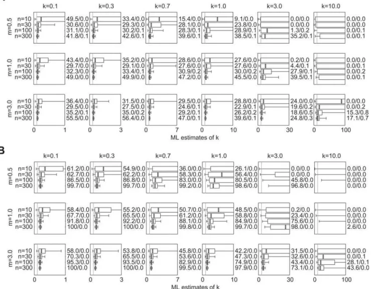
The results for NB surveillance datasets subject to uniform under-counting are shown in Figure 2. Results are shown for two values of the probabilityputhat any given secondary case is missed by surveillance. When pu= 0.2 (Fig. 2a), estimates of kˆ from these datasets differed only slightly from estimates from raw NB data (Fig. 1), exhibiting all the same qualitative patterns and slightly worse bias and precision. Whenpu= 0.5 (Fig. 2b), results exhibited similar, but more extreme, differences from the raw NB results.
3.3 Negative binomial data with under-reporting of
zeroes
Results of estimation from NB surveillance datasets with under-reporting of the zero class, in which individuals who causedxi= 0 cases were omitted from simulated datasets with probabilitypz, are shown in Figure 3. For bothpz= 0.2 (Fig. 3a) andpz= 0.5 (Fig. 3b), estimates ofkˆare biased upward significantly. Notably, this effect does not diminish as sample size increases. Indeed, for most para-meter sets the proportion of CI overestimates increases with higher
3.4 Outbreak data
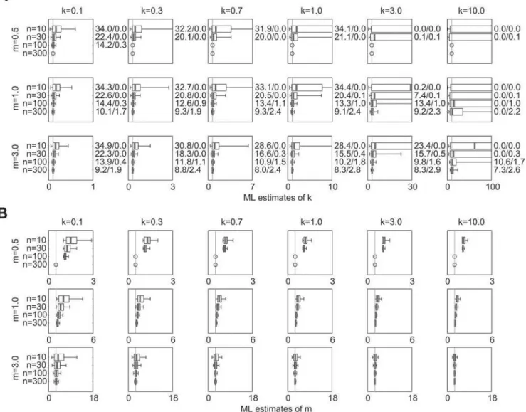
Estimates from simulated outbreak datasets are shown in Figure 4. Form= 0.5 andk.0.1, no results are presented forn$100 because
fewer than 1 in 105simulated outbreaks reached 100 cases. For
other values ofmandk, estimates ofkˆare quite robust (Fig. 4a). Comparing these results to estimates from Figure 1, it is evident that estimates from outbreak datasets have similar biases (slightly positive for smalln, but diminishing asnincreases) and precisions that are as good and sometimes better than those from unaltered NB data. The outbreak datasets yield slightly more CI over-estimates form= 3, even though the IQR and [5th, 95th] percentile interval of the sampling distribution is often smaller. Outbreak datasets yield fewer CI overestimates for k= 0.1, m= 0.5 or 1.0, andn= 10 or 30.
ML estimates of the mean are shown for these datasets as well (Fig. 4b). There is a striking positive bias evident in the estimates of
mˆ form= 0.5; in all cases shown, the distribution ofmˆ estimates has median value.1 and 5thpercentile value$1. Form= 1, there is an upward bias in the mˆ estimates that decreases as sample size rises. For m= 3, the upward bias persists but is very slight for
k$0.3 orn$30.
DISCUSSION
This study makes three novel contributions to the established
literature on estimation of the NB dispersion parameter k. It
provides the first comprehensive evaluation of ML estimation ofk
for highly overdispersed datasets (i.e. those withk,1); it reports the coverage accuracy of CIs derived from those estimates; and it examines potential biases in estimation due to methods and errors of data collection, with application to epidemiological datasets in particular and biological datasets in general. The major qualitative results are summarized in Table 1.
The results for unaltered NB datasets confirm and extend the findings of earlier studies. Small-sample estimates ofkˆwere biased
toward overestimatingk—and hence underestimating the degree
of overdispersion in the data—as reported in previous studies using
ML and related methods of estimation fork$1 [14,15,17]. The
positive bias inkarises because smaller samples are less likely to include values from the right-hand tail of the NB distribution, without which the dataset appears more homogeneous. Estimates
of kˆ were less biased and more precise for larger values of m,
possibly because such datasets had higher total numbers of non-zero events. Estimates were more biased and less precise for higher values ofk (particularly in the previously-studied range ofk$1), corresponding to the known instability of ML estimates when data are closer to being fitted by a Poisson distribution [13]. Intuitively, this effect arises because a NB distribution withk= 10 is qualita-tively similar to one withk= 50 or kR‘, and quite dissimilar to one withk= 1, so the range ofkˆestimates for small samples tends to be large and skewed upwards.
One previous simulation study [16] presented in-depth results for estimation ofk,1 (specifically, fork= 0.4), employing
method-of-moments estimateskˆmomrather than the ML estimates assessed
here. That study reported that smaller sample sizes from NB datasets led to systematic underestimation of the mean and
variance and overestimation ofk; the variance/mean ratio was
also biased downward by smalln. There is one interesting differ-ence between the method-of-moments estimates results of Gregory and Woolhouse [16] and the present results for ML estimation: the positive bias ofkˆmomwas fairly constant asmincreased (though the range ofkˆmomvalues was greatest for lowerm), while the bias of ML estimateskˆdecreased for higherm(Fig. 1). It is notable that their values ofmranged from 1.25 to 160 (fork= 0.4), while the values used here ranged from 0.5 to 3 (forkbetween 0.1 and 10). Several salient patterns emerged regarding the realized coverage of 90% CIs, as estimated using the asymptotic variance of ML estimates. The true coverage of the nominal 90% intervals was typically less than 90%, and CI overestimates were much more numerous than CI underestimates. For all parameter sets con-sidered,,5% of CIs had upper bounds below the true value ofk. The realized coverage of the CIs is driven by the interplay of two factors: the value of the estimates,kˆ, and the breadth of the intervals (determined by the sampling variance,s2^
k
k). The upward bias ofkˆincreases for lower values ofnandmand higher values of
Figure 1.Estimated values ofkˆand confidence interval coverage for NB datasets. 10,000 datasets were simulated as described in Section 2.1.1 of the text, using meanm, dispersion parameterk, and sample sizenas shown. Boxes show the median and interquartile range (IQR) of 10,000 resulting ML estimates ofkˆ, and whiskers show the 5thand 95thpercentile values. Numbers to the right of each subplot show the percentage of simulations for which the true value ofkwas outside (below (CI overestimate)/above (CI underestimate) for the numbersy/z, respectively) the 90% confidence interval estimated forkˆThe vertical line in each subplot shows the true value ofk. To facilitate comparison among parameter sets, the horizontal axis of all subplots is scaled from 0 to 10 times the true value ofk.
k; lower values of n, m, or k lead to increases in s2^
k and hence
broader intervals. Overestimates of kˆ favor CI overestimates by
setting a high mid-point for the estimated intervals, and by reducing the estimated sampling variance (becauses^2
kis calculated with an inflated value ofk) and thus leading to narrower intervals. The gross patterns in the frequency of CI overestimates thus are driven primarily by patterns of bias inkˆ.
To understand the finer patterns in CI coverage accuracy, particularly for CI underestimates and for CI overestimates for
higher values of k, it is necessary to consider how the CIs are
calculated. Recall that intervals were estimated for a= 1/k as
[aˆ2z0.95saˆ, aˆ+z0.95saˆ], then converted into intervals for k. CI
underestimates for k occur when a,aˆ2z0.95saˆ. The complete
absence of CI underestimates in many small-n parameter sets
arises becauseaˆ,z0.95saˆsuch that the lower bound of the CI foraˆ
is,0. In these instances, the upper bound of the CI forkˆis set to
the maximum value forkˆand cannot be exceeded. Asn,m, ork
increases, saˆ decreases and the CIs narrow such that some CI
underestimates occur. Similarly, CI overestimates occur when
a.aˆ+z0.95saˆ. As k increases, CI overestimates become less
frequent (despite the high frequency ofkˆ overestimates) because a= 1/kis often smaller thanz
0.95saˆ. Becauseaˆ is constrained to
positive values in these simulations, CI overestimates are impossible when a,z0.95saˆ. Accordingly, for given values of
k.1, CI overestimates are more frequent for higher values ofnand
m(corresponding to lower values of saˆ). This study’s focus on
overdispersed datasets, and hence on the positive values of k
familiar to biologists, has thus influenced the determination of CI coverage in some regions of parameter space. Estimation
procedures allowing for underdispersed data (aˆ,0) may show
different results. Investigators requiring CIs guaranteed to reach nominal levels of coverage should consult the literature on exact CIs for discrete distributions [e.g. 26].
The simulation results from surveillance and outbreak datasets (Figs. 2–4) can be interpreted readily in light of the raw NB results discussed above. For datasets where individual values correspond to completely unconnected events (e.g. epidemiological surveil-lance of multiple independent introductions of a disease, or many
Figure 2.Estimated values ofkˆand confidence interval coverage for NB datasets with uniform under-counting of secondary cases. The probability with which any secondary case was missed by surveillance was (a)pu= 0.2 and (b)pu= 0.5. 10,000 datasets were simulated as described in Section 2.1.2 of the text, for parametersm,k, andnas shown. Plotting details are described in Figure 1.
other biological observations), the effects of two forms of under-reporting were assessed. In uniform under-counting, each instance of the quantity being counted (e.g. secondary cases, in the epidemiological context) can be overlooked with equal probability
pu. The expected value of each datumxiin the raw dataset (drawn
from an NB distribution with parametersmandk) is reduced to
(12pu) xi, and the resulting distribution is NB with parameters (12pu) mand k (as argued under the topic of ‘population-wide control measures’ by Lloyd-Smith et al. [8]). Thus uniform under-counting does not introduce systematic bias to ML estimates ofk, but does cause a slight increase in the small-sample bias and decrease in precision (Fig. 2) corresponding to the effect of a lower mean, as characterized for raw NB data (Fig. 1).
In contrast, the second class of under-reporting bias, in which
xi= 0 events are omitted from datasets with probabilitypz, leads to systematic overestimation ofkthat does not vanish asnincreases (Fig. 3). NB distributions with lowkare characterized by large zero classes and long tails (giving rise to the large variance-to-mean ratios that define overdispersion). Decreasing the proportion of zeroes (hence replacing xi= 0 events by xi.0 events) leads to
higher sample meanmˆ and lower sample variancesˆ2. As is readily
seen from the method-of moments estimator kˆmom=mˆ
2
/(sˆ22mˆ) [10], this will bias estimates ofk to higher values. Investigators should be vigilant for this class of under-reporting bias, and conduct estimation using a zero-modified NB distribution [27] if zero under-counting is suspected.
Outbreak datasets involve a mechanism of data generation that is particular to epidemiological (or demographic) processes. Earlier analyses have shown that when offspring distributions are highly overdispersed (e.g. NB withk,1), the outbreaks that succeed tend to be those with early superspreading events [8]. The present results show that this does not cause underestimation ofkas had been feared; estimates ofkˆfrom outbreak data (Fig. 4a) exhibited similar properties to those from raw NB data (Fig. 1). Indeed, outbreak estimates had slightly smaller bias and greater precision for smallern, probably because the use of outbreak data (biased
toward including high-xi events) counteracts the usual
small-sample bias (which arises because small datasets often lack high-xi events). Therefore the selection bias inherent in outbreak datasets acts to offset somewhat the usual upward bias in estimates ofkˆ.
Figure 3.Estimated values of kˆ and confidence interval coverage for NB datasets with under-reporting of zeroes. Individuals that caused no secondary infections were missed by surveillance with probability (a)pz= 0.2 and (b)pz= 0.5. 10,000 datasets were simulated as described in Section 2.1.3 of the text. Plotting details are described in Figure 1.
In sharp contrast, estimation of mˆ from outbreak datasets (assessed by simulation because, unlike the surveillance cases, the potential bias cannot be computed directly) is strongly biased
upward whenmis below or near 1 (Fig. 4b). This is unsurprising
because the minimum value ofmˆ for an outbreak withncases is
(n21)/n(for an outbreak that dies out immediately following the
nth case), while higher values are quite feasible. (Recall thatmˆ is estimated as the mean number of secondary cases generated by the
first ncases in an outbreak, regardless of whether the outbreak
continues beyondncases. If the cumulative number of cases after therthgeneration of transmission isj, then the mean value ofxifor
i= 1 to j is (j21)/j. If the nth case then occurs in the (r+1)th generation of transmission, then all infections caused by the final
n2jindividuals in the dataset (i.e.xifori=j+1 ton) serve to inflate
mˆ above its minimum value of (n21)/n.) The greatest bias in mˆ
occurs for lowkand n, when large superspreading events in the
final generation can have disproportionate effect on the sample
mean. For m= 1.0, the bias decreases as n increases, probably
because higher-n datasets involve more generations of disease
transmission, so the ‘left-over’ cases of the final generation (i.e. the
final n2j individuals in the example above) make a smaller
proportional contribution. Form= 3.0, there is no substantial bias for any parameters (with a minor exception fork= 0.1 andn= 10). The results presented here suggest several avenues for future work. This study has focused on ML estimation only, and it would
Figure 4.Estimated values of (a)kˆand (b)mˆ for outbreak datasets generated by branching process simulations with NB offspring distributions. 10,000 datasets were simulated as described in Section 2.1.4 of the text. Circles indicate parameter sets for which fewer than 1 in 105simulated outbreaks hadncases or more. Other plotting details are described in Figure 1.
doi:10.1371/journal.pone.0000180.g004
Table 1.Influence of NB parameters and data types on bias
and precision ofkˆ.
. . . .
For increasing values of these parameters:
For outbreak data
n k m pu pz
Lower bias + + 2 + 2 2 2* +
Higher precision + + 2 + 2 2 +
+indicates lower bias or higher precision
2indicates larger upward bias or lower precision
*
indicates systematic bias that does not vanish asnR‘
doi:10.1371/journal.pone.0000180.t001
....
...
....
...
...
....
...
...
....
...
...
....
be fruitful to extend the conclusions to other methods of estimating
k, such as maximum quasi-likelihood [14], method-of-moments
with small-sample correction [16], or bias-corrected ML [17]. Further studies on estimation ofmˆ will be interesting, particularly in the epidemiological context where the mean of the offspring distribution is equivalent to the crucial quantity R0 [8,22]. In
particular, it will be important to learn how the overdispersion observed in disease transmission data [8] influences estimation of
R0from continuous-time outbreak data such as daily case reports
[28,29], as opposed to estimation directly from known chains of transmission as assessed here. Overdispersed offspring distribu-tions cause outbreaks to either die out stochastically or grow
explosively [8], so estimation of R0 from daily case reports (of
successful outbreaks only, necessarily) may exhibit bias beyond that shown in Figure 4b.
In summary, this study showed that there is minimal risk of
underestimating k—and hence of overestimating the degree of
overdispersion in the data—due to small sample size or any of the three process biases considered here. There is substantial risk of overestimatingk, particularly when sample sizes are small or the zero-class is systematically under-counted. All of the systematic biases identified in this study favored higher values of kˆ, and instances when confidence intervals excluded the true valuekwere
predominantly overestimates. Note that an independent risk of
underestimatingkcan arise from pooling data from heterogeneous
groups: the dispersion parameter estimated from pooled data is nearly always less than the average of values estimated for the individual groups [11,16]. Regarding sample sizes for NB datasets
with k#1, n= 100 or more allows accurate and precise ML
estimation of kˆ, while for n= 30 the median estimates showed
minimal bias but the sampling distribution skewed to high values. A sample size of 10 yields unreliable estimates, particularly for
m#1. These findings will help guide prospective design of
sampling regimens, or, when sample size cannot be increased, will aid investigators in understanding the limitations of ML estimates ofkˆand associated CIs.
ACKNOWLEDGMENTS
I am grateful to Leo Polansky, Sadie Ryan and Maria Sanchez for helpful comments on the manuscript.
Author Contributions
Conceived and designed the experiments: JL. Performed the experiments: JL. Analyzed the data: JL. Contributed reagents/materials/analysis tools: JL. Wrote the paper: JL.
REFERENCES
1. Bliss CI, Fisher RA (1953) Fitting the negative binomial distribution to biological data - note on the efficient fitting of the negative binomial. Biometrics 9: 176–200.
2. Pielou EC (1977) Mathematical Ecology. New York: Wiley.
3. White GC, Bennetts RE (1996) Analysis of frequency count data using the negative binomial distribution. Ecology 77: 2549–2557.
4. Shaw DJ, Grenfell BT, Dobson AP (1998) Patterns of macroparasite aggregation in wildlife host populations. Parasitology 117: 597–610.
5. Walther BA, Morand S (1998) Comparative performance of species richness estimation methods. Parasitology 116: 395–405.
6. Power JH, Moser EB (1999) Linear model analysis of net catch data using the negative binomial distribution. Can J Fish Aq Sci 56: 191–200.
7. Alexander N, Moyeed R, Stander J (2000) Spatial modelling of individual-level parasite counts using the negative binomial distribution. Biostatistics 1: 453–463. 8. Lloyd-Smith JO, Schreiber SJ, Kopp PE, Getz WM (2005) Superspreading and the effect of individual variation on disease emergence. Nature 438: 355–359. 9. Harris TE (1989) The Theory of Branching Processes. New York: Dover. 10. Anscombe FJ (1950) Sampling theory of the negative binomial and logarithmic
series distributions. Biometrika 37: 358–382.
11. Pieters EP, Gates CE, Matis JH, Sterling WL (1977) Small sample comparison of different estimators of negative binomial parameters. Biometrics 33: 718–723. 12. Wilson K, Bjornstad ON, Dobson AP, Merler S, Poglayen G, et al. (2001)
Heterogeneities in macroparasite infections: patterns and processes. In: Hudson PJ, Rizzoli A, Grenfell BT, Heesterbeek H, Dobson AP, eds. The Ecology of Wildlife Diseases. Oxford: Oxford University Press. pp. 6–44. 13. Ross GJS, Preece DA (1985) The negative binomial distribution. Statistician 34:
323–336.
14. Clark SJ, Perry JN (1989) Estimation of the negative binomial parameter kappa by maximum quasi-likelihood. Biometrics 45: 309–316.
15. Piegorsch WW (1990) Maximum-likelihood estimation for the negative binomial dispersion parameter. Biometrics 46: 863–867.
16. Gregory RD, Woolhouse MEJ (1993) Quantification of parasite aggregation -a simul-ation study. Act-a Trop 54: 131–139.
17. Saha K, Paul S (2005) Bias-corrected maximum likelihood estimator of the negative binomial dispersion parameter. Biometrics 61: 179–185.
18. Thompson WL (2002) Towards reliable bird surveys: Accounting for individuals present but not detected. Auk 119: 18–25.
19. Wallinga J, Teunis P (2004) Different epidemic curves for severe acute respiratory syndrome reveal similar impacts of control measures. Am J Epidemiol 160: 509–516.
20. Gray BR (2005) Selecting a distributional assumption for modelling relative densities of benthic macroinvertebrates. Ecol Model 185: 1–12.
21. Donnelly CA, Fisher MC, Fraser C, Ghani AC, Riley S, et al. (2004) Epidemiological and genetic analysis of severe acute respiratory syndrome. Lancet Infect Dis 4: 672–683.
22. Diekmann O, Heesterbeek JAP (2000) Mathematical Epidemiology of Infectious Diseases: Model Building, Analysis, and Interpretation. Chichester: John Wiley & Sons.
23. Boswell MT, Patil GP (1970) Chance mechanisms generating the negative binomial distribution. In: Patil GP, ed. Random Counts in Scientific Work. University ParkPA: Pennsylvania State University Press. pp. 3–22.
24. Rice JA (1995) Mathematical statistics and data analysis. Belmont, CA: Duxbury Press.
25. Willson LJ, Folks JL, Young JH (1984) Multistage estimation compared with fixed-sample-size estimation of the negative binomial parameterk. Biometrics 40: 109–117.
26. Blaker H (2000) Confidence curves and improved exact confidence intervals for discrete distributions. Can J Stat 28: 783–798.
27. Ridout MS, Demetrio CGB, Hinde JP (1998) Models for counts data with many zeros. Proceedings of the XIXth International Biometric Conference. pp. 179–192.
28. Anderson RM, May RM (1991) Infectious Diseases of Humans: Dynamics and Control: Oxford University Press.
29. Ferrari MJ, Bjornstad ON, Dobson AP (2005) Estimation and inference ofR0of