DOI: 10.2298/SAJ1590041B Original scientific paper
TIMELIKE GEODESICS AROUND A CHARGED SPHERICALLY
SYMMETRIC DILATON BLACK HOLE
C. Blaga
Faculty of Mathematics and Computer Science, Babe¸s-Bolyai University Cluj-Napoca Kog˘alniceanu Street 1, Cluj-Napoca, Romania
E–mail: [email protected]
(Received: December 29, 2014; Accepted: March 3, 2015)
SUMMARY: In this paper we study the timelike geodesics around a spherically symmetric charged dilaton black hole. The trajectories around the black hole are classified using the effective potential of a free test particle. This qualitative ap-proach enables us to determine the type of orbit described by test particle without solving the equations of motion, if the parameters of the black hole and the par-ticle are known. The connections between these parameters and the type of orbit described by the particle are obtained. To visualize the orbits we solve numerically the equation of motion for different values of parameters envolved in our analysis. The effective potential of a free test particle looks different for a non-extremal and an extremal black hole, therefore we have examined separately these two types of black holes.
Key words. black hole physics – gravitation – relativistic processes
1. INTRODUCTION
In classical general relativity the geometry of the spacetime near a charged black hole is described by Reissner-Nordstrøm metric. In the low-energy string theory, the solution for a static charged black hole was obtained by Gibbons and Maeda (1988) and three years later, independently, by Garfinkle, Horowitz and Strominger (1991). Thus the static spherically symmetric charged dilaton black hole is known as Gibbons–Maeda–Garfinkle–Horowitz– Strominger (GMGHS) black hole.
In 1993, using a Harrison-like transforma-tion (Harrison 1968) to the Schwarzschild solu-tion, Horowitz (1993) derived a metric that fulfills Einstein-Maxwell field equations. For a massless dilaton the solution found by Horowitz corresponds to a GMGHS black hole.
The line element of the metric is:
ds2=− µ
1−2M
r
dt2+ 1 ¡
1−2M r
¢dr 2
+r
µ
r−Q
2
M
(dθ2+ sin2
θ dϕ2), (1)
whereQis related to electrical charge of a black hole and M to its mass. If Q2 < 2M2 the singularity is inside the event horizon. If Q2 = 2M2, the area of the event’s horizon shrinks to zero. This case is known asthe extremal limit.
In classical general relativity as well as in string theory, geodesics of black holes are studied extensively. The critical parameters for photon and timelike geodesics for Kerr black holes and Reissner-Nordstrøm black holes have been found from condi-tions for multiple roots of corresponding polynomi-als by Zakharov (1994, 2014) and Zakharov et. al. (2005a,b, 2014). The null geodesics of static charged black holes in heterotic string theory were analysed by Fernando (2012). The circular null and timelike geodesics for a non-extremal and extremal GMGHS black hole were investigated by Pradhan (2012). The exact solutions of timelike geodesics of an extremal GMGHS black hole were derived in Blaga and Blaga (1998). The existence and stability of circular or-bits for the timelike geodesics of a GMGHS black hole were examined in Blaga (2013). A quantitative analysis of the timelike geodesics of a charged black hole in heterotic string theory was done by Olivares and Villanueva (2013), article in which the authors obtained the solution of geodesic equations in terms of elliptic℘-Weierstrass function.
Our goal is to classify the orbits of free test particles in the vicinity of a spherically symmetric dilaton black hole using the effective potential. This approach enables us to identify the type of orbit de-scribed by a particle around a GMGHS black hole without solving the equations of motion. The type of the orbit described by a free test particles around a given GMGHS black hole depends on its angular momentum, energy and initial position. The qual-itative results are accompanied by plots of possible orbits described by free test particles around differ-ent GMGHS, obtained by numerical integration of the equations of motion. The initial condition for a given type of black hole was chosen using the knowl-edge about peculiarities of the effective potential.
The paper is organized as follows: in Section 2 we derive the geodesic equations from the Lagrangian corresponding to metric Eq. (1). In Section 3 we emphasize some properties of the effective potential of a free test particle for both a non-extremal and extremal GMGHS. In Section 4 we classify the pos-sible trajectories around a GMGHS black hole with
b ∈[0,2), respectively b= 2 and plot the numerical solution of the geodesic equations for different val-ues of the parameters involved in our analysis. The conclusion are given in the last section.
2. GEODESIC EQUATIONS
We can derive the geodesic equations by di-rectly computing the Christoffel coefficients for the given metric or by using Hamilton-Jacobi theory (see for example Blaga and Blaga 1998) or by writing the Euler-Lagrange equations (see Fernando 2012). We follow here the later approach described by Chan-drasekhar (1983). The Lagrangian for the metric Eq. (1) is:
2L=−
µ 1−2M
r
¶ ˙
t2+ µ
1−2M
r
¶−1 ˙
r2
+r
µ
r−Q
2
M
¶³ ˙
θ2+ sin2θϕ˙2´, (2)
where the dot means the differentiation with respect toτ - the affine parameter along the geodesic. This parameter is chosen so that 2L =−1 on a timelike geodesic, 2L= 0 on a null geodesic and 2L= 1 on a space-like geodesic.
The coordinates t and ϕ are cyclic. There-fore the motion has two first integrals derived from the Euler-Lagrange for time and latitude as follows. From the Euler-Lagrange equation fortwe get:
µ 1−2M
r
¶ ˙
t= E , (3)
known as the energy integral. The real constantEis the total energy of the particle. The second integral of motion is obtained from the Euler-Lagrange forϕ:
2r
µ
r−Q
2
M
sin2θϕ˙ = constant, (4)
known as the integral of angular momentum. From the Euler-Lagrange equation for θ we get:
d dτ
·
r
µ
r−Q
2
M
¶ ˙
θ
¸ =r
µ
r−Q
2
M
sinθcosθ·ϕ˙2.
(5) Considering θ = π/2 when ˙θ = 0, then ¨θ = 0 and
θ=π/2 on geodesic. This means that the motion is confined in a plane as in the Schwarzschild spacetime or in Newtonian gravitational field.
Ifθ=π/2 during the motion the angular mo-mentum integral Eq. (4) becomes:
r
µ
r−Q
2
M
¶ ˙
ϕ=L , (6)
where the real constantLis the angular momentum about an axis normal to the plane in which the mo-tion took place.
The Euler-Lagrange equation corresponding to the radial coordinate is complicated. Therefore, we replace it with a relation derived from the con-stancy of the Lagrangian. If we substitute in Eq. (2)
˙
t from Eq. (3), ˙ϕfrom Eq. (6) and ˙θfrom Eq. (5), after some algebra we get:
µ
dr dτ
¶2 +
µ 1−2M
r
L2
r³r−Q2
M ´−ǫ
=E 2
,
2.1. Radial timelike geodesics
The angular momentum of a free test particle moving on a radial timelike geodesics is zero. There-fore Eq. (7) becomes:
µ
dr dτ
¶2 +
µ 1−2M
r
=E2. (8)
If we want to study the motion of a test particle which describes a radial timelike geodesic we have to consider Eq. (8) for radial coordinate r and the Euler-Lagrange equation for time coordinatet:
dt dτ =
E
¡ 1−2M
r
¢, (9)
where τ is the proper time. These two equations are identical with the equations of radial timelike geodesics in the Schwarzschild spacetime (Chan-drasekhar 1983). Therefore, the motion of free test particles on radial geodesics in the vicinity of these two kind of black holes will have the same properties. It is well known that an observer stationed at a large distance from a Schwarzschild black hole finds that a free falling test particle approaches to events horizon but can never cross it, because the test particle needs an infinite time t to reach the horizon even though it crosses the horizon in a finite proper time τ. This property is valid for a free falling particle on a radial timelike geodesic of GMGHS black holes, too.
3. EFFECTIVE POTENTIAL FOR TIMELIKE GEODESICS
If we compare Eq. (7) with ˙r2+V
eff=E2 we get the effective potential:
Veff= µ
1−2M
r
L2
r³r−QM2´ −ǫ
, (10)
which depends on radial coordinate r, the parame-ters related to the electrical charge and mass of the black hole, the type of the geodesics and the angular momentum of the particle.
For timelike geodesics ǫ = −1 and Eq. (10) becomes
Veff = µ
1−2M
r
L2
r³r−QM2´
+ 1
. (11)
In order to lower the number of parameters from the effective potential we denoteu=r/M,a= (L/M)2,
b= (Q/M)2 and the Eq. (11) becomes:
Veff= µ
1−2
u
¶ µ a
u(u−b)+ 1 
. (12)
The quantity q = Q/M is the specific electrical charge and we observe that b = q2. In this paper we have assumed that Q2 ≤ M2 hence b ∈ [0,2], where b = 0 is for a Schwarzschild black hole and
b= 2 for an extremal GMGHS black hole. The pa-rameter aequals (L/M)2, therefore in our study it will be positive or zero. In the new variable u, the events horizon corresponds to u= 2 and the region outside the horizon will be given byu >2.
3.1. Effective potential for
b∈[0,2)
The effective potential Eq. (12) was studied in Blaga (2013). The qualitative analysis ofVeff re-vealed that forb∈[0,2), the function is positive for
u∈[2,+∞), it is zero on the events horizon u= 2 and approaches 1 asuapproaches +∞(see Fig. 1). Ifais greater then a value depending onb(see Blaga 2013), the potential has two local extreme points out-side the events horizon, the local maximum point of
Veff being closest to the horizon. For a given b, if there is a local maximum point outside the horizon, the maximum value of the potential increases with
a.
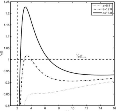
In Fig. 1 we have plotted the effective poten-tial against u=r/M for b = 1 and three values of
a. The first valuea= 8.41054 is the lowest value of
a for which Veff admits extreme points outside the horizon forb= 1 (see Blaga 2013). The second value
a= 12 is the lowest value ofafor which the effective potential admits extreme points outside the horizon in the case of a Schwarzschild black hole b= 0 (see Chandrasekhar 1983).
2 4 6 8 10 12 14 16 0.8
0.85 0.9 0.95 1 1.05 1.1 1.15 1.2 1.25
Veff+∞
u=r/M Veff
a=8.41 a=12.0 a=16.0
Fig. 1. Effective potential for b = 1 and a ∈ {8.41,12,16}. The dashed lines are for the vertical
u= 2 - events horizon and horizontalVeff = 1 - the limit of the potential asu→+∞.
If we choose another value for b ∈ [0,2) dif-ferent from 1, the graph of the effective potential is similar, but for a given value ofa, if the potential ad-mits two extreme points outside the events horizon, the maximum value of the potential increases withb
3.2. Effective potential for b= 2
For a test particle moving around an extremal GMGHS black hole b= 2 the effective potential is:
Veff(u) =u
2−2u+a
u2 , (13)
a function which is not defined in u= 0, approaches infinity as uapproaches zero and 1 asuapproaches infinity (see Fig. 2). In this case the effective po-tential admits only a local minimum point inu=a. This point is outside the events horizon if and only if a ≥ 2. The minimum value of the effective po-tential increases with a, it approaches 1 from below as a approaches +∞. We have plotted the effective potential Eq. (13) for various values of ain Fig. 2.
2 4 6 8 10 12 14 16 0.8
0.85 0.9 0.95 1 1.05 1.1 1.15 1.2 1.25
Veff+∞
u=r/M Veff
a=8.41 a=12.0 a=16.0
Fig. 2. Effective potential for b = 2 and
a∈ {8.41,12,16}. The dashed lines are for the ver-tical u= 2 - events horizon and horizontalVeff= 1 -the limit of -the potential asu→+∞.
4. TYPES OF TIMELIKE GEODESICS
If we replace ε = −1 in Eq. (7) we get the equation of motion of a free test particle around a spherically symmetric charged black hole. Therefore, the geometry of the orbit described by the test par-ticle depends on its energy.
The motion is possible only ifE2−Veff(u)≥0. The points in whichE2=Veff(u) are known as turn-ing points because dr/dt = 0 and the direction of motion could be changed there.
-4.1. Orbits around a dilaton black hole with b∈[0,2)
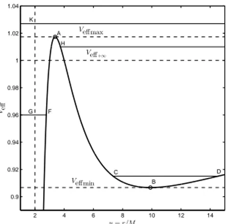
In Fig. 3 we have plotted the effective poten-tial for a dilaton black hole with b= 1 as an expo-nent for GMGHS black holes with b ∈ [0,2). The parameter a = 12. The points A and B represent the maximum, and minimum point of the effective potential respectively. The dashed horizontal lines
are for the maximum value of potentialVeffmax, the minimum value Veffmin and the limit of the poten-tial asuapproaches infinityVeff+∞. The horizontal solid lines represent different energy levels. C, D,F
andH denote the intersection points of energy level with the graph of the effective potential. The points in which a test particle crosses the line u = 2 are denoted byGandK.
2 4 6 8 10 12 14 0.9
0.92 0.94 0.96 0.98 1 1.02 1.04
Veff+∞
A Veffmax
B Veffmin
K
H
G F
C D
u=r/M Veff
Fig. 3. Effective potential for b = 1 and a= 12. Dashed lines are for the extreme values of the ef-fective potential, the limit of the potential as u ap-proaches infinityVeff+∞ and the verticalu= 2. The solid lines are for different energy levels.
If we consider a free test particle moving around a dilaton black hole with b ∈ [0,2) and a
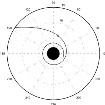
greater then the lower value for which the effective potential has extrema outside the events horizon, the graph of the effective potential is similar to the graph in Fig. 3. The reason why we have computed the or-bits around a GMGHS black hole with b = 1 is to visualize the geometry of possible trajectories around GMGHS black holes with an arbitraryb∈[0,2). In the following polar plots we have represented the re-gion inside events horizon as a circle filled with black. The orbits were obtained by numerical integration of Eq. (7) and Eq. (6) usingMatlab.
If the motion of a free test particle around a dilaton black hole is possible then, depending on the total energy of the test particle and its initial position
u0, we can find the following qualitative motions: Case 1: ifE2> V
effmaxthen the test particle approaches the black hole, crosses the events hori-zon and ends into the singularity. The particle is gravitationally captured.
In Fig. 4 we have represented a gravitational capture. The free test particle is moving with the to-tal energy corresponding to the highest energy from Fig. 3, crosses the events horizon inK and end into the singularity.
Case 2: if E2 ∈ (1, Veffmax), u
5 10
15
30
210
60
240
90
270 120
300 150
330
180 0
Fig. 4. Gravitational capture. Here a= 12,b= 1,
E2= 1.03andu
0= 15.0.
5 10
15
30
210
60
240
90
270 120
300 150
330
180 0
Fig. 5. Hyperbolic scattering. Here a= 12,b= 1,
E2= 1.01
andu0= 15.0.
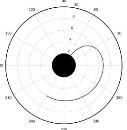
In Fig. 5 we have represented the orbit of a test particle with an energy equal to the energy from the second energy level from Fig. 3. In H the test particle change its direction of motion and turns back to large distances from the black hole.
Case 3: if E2=V
effmax andu0=u(A) then the test particle describes a circular orbit around the black hole (see Fig. 6). Since Ais a local maximum point for effective potential the circular orbit is un-stable.
5 10
15
30
210
60
240
90
270 120
300 150
330
180 0
Fig. 6. Unstable circular motion. Here a = 12,
b= 1,E2= 1.073 andu
0= 3.381.
Case 4: if E2 =Veffmax, u
0 > u(A) and the motion is possible, the particle escapes to infinity. We say that it is moving on an outer marginal orbit (see Fig. 7). If E2 = V
effmax and u0 < u(A), the particle ends into the singularity and we say that it describes an inner marginal orbit (see Fig. 8).
5 10
15
30
210
60
240
90
270 120
300 150
330
180 0
Fig. 7. Outer marginal orbit. Here a= 12,b= 1,
E2= 1.073,u
0= 3.39.
5 10
15
30
210
60
240
90
270 120
300 150
330
180 0
Fig. 8. Inner marginal orbit. Herea= 12, b= 1,
E2= 1.073,u
0= 3.37.
Case 5: ifE2 < Veffmax,u
0 < u(A) and mo-tion is possible then the test particle moves toward the singularity crossing the horizon inF (see Fig. 9). Motion is trapped near the horizon.
Case 6: if E2 ∈ (V
effmin,min(1, Veffmax)),
u0 > u(A) and motion is possible then the test particle moves toward and backward from the black hole. C and D are the points where the test par-ticle changes its direction of motion. The orbit is bounded and the motion is restricted in the annular region placed between the circles with radius u(C) andu(D), respectively.
2 4
6 8
30
210
60
240
90
270 120
300 150
330
180 0
Fig. 9. Motion trapped near the horizon. Here
a= 12,b= 1,E2= 0.96,u
0= 2.75.
5 10
15 20
30
210
60
240
90
270 120
300 150
330
180 0
Fig. 10. Bounded orbit. Here a = 12, b = 1,
E2= 0.915,u
0= 7.5,u(C) = 7.355,u(D) = 14.53.
Case 7: if E2 = V
effmin and u0 = u(B) the test particle describes a stable circular orbit, because
B locates the minimum point of effective potential (see Fig. 11).
5 10
15
30
210
60
240
90
270 120
300 150
330
180 0
Fig. 11. Stable circular orbit. Herea= 12,b= 1,
E2= 0.907,u 0= 9.9.
The unstable and stable circular orbits are in fact specially bounded orbits with u = u(A) and
u=u(B), respectively.
We notice that the type of trajectories enu-merated in this section are qualitatively similar to the trajectories found in a Schwarzschild spacetime (see Frolov and Zelnikov 2011). This fact was expected because a Schwarzschild black hole is a GMGHS black hole with b = 0. The difference be-tween the orbits around a Schwarzschild black hole and a GMGHS dilaton black hole with b ∈ (0,2) appears in dynamical parameters of motion. For ex-ample, for a givenathe test particle needs a higher energy to be gravitationally captured because the maximum value of the effective potential increases withb.
4.2. Trajectories around an extremal GMGHS black hole
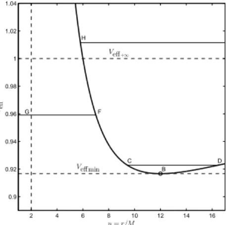
In Fig. 12 we have plotted the effective po-tential for an extremal dilaton black hole for a = 12. The horizontal dashed lines are for the mini-mum value of effective potential and its limit when
u→ +∞. The vertical u= 2 plotted with dashed line corresponds to the events horizon. The energy levels are represented with solid lines. The pointB
is the minimum point of the effective potential, C,
D,F andH are the turning points andGthe point in which the test particles cross the horizon.
2 4 6 8 10 12 14 16 0.9
0.92 0.94 0.96 0.98 1 1.02 1.04
Veff+∞
B Veffmin
H
G F
C D
u=r/M Veff
Fig. 12. Effective potential for b= 2. The dashed lines are for the minimum value of the effective po-tential, the limit of the potential asuapproaches in-finityVeff+∞ and the vertical u= 2. The solid lines are for different energy levels.
If we consider a free test particle moving around an extremal dilaton black hole b = 2 and
a ≥ 2, then the graph of the effective potential is similar to the plot from Fig. 12. Depending on total energy of the particle and its initial positionu0a free test particle describes one of the following trajecto-ries:
Case 1: if E2 ≥ 1 and u
0 > u(H), where
5 10
15
30
210
60
240
90
270 120
300 150
330
180 0
Fig. 13. Hyperbolic scattering. Herea= 12,b= 2,
E2= 1.012,u
0= 15.0.
Case 2: if E2 > V
effmin and u = r/M0 <
u(F), whereF is a solution of the equationVeff(u) =
E2, the particle falls into the singularity, crossing the horizon in G. In this case the orbit is trapped near the events horizon. In Fig. 14 the total energy of the test particle corresponds to the second energy level from Fig. 12.
2 4
6 8
10
30
210
60
240
90
270 120
300 150
330
180 0
Fig. 14. Near the horizon trapped motion. Here
a= 12,b= 2,E2= 0.96,u 0= 6.0.
5 10
15 20
30
210
60
240
90
270 120
300 150
330
180 0
Fig. 15. Bounded orbit. Here a = 12, b = 2,
E2= 0.922, u
0= 9.45. The dashed lines are for the circles u(C) = 9.43andu(D) = 16.49.
Case 3: ifE2 ∈ (V
effmin,1) and u0 > 2 the particle moves toward and backward from the black hole. The particle changes its direction of motion in the turning points C and D, respectively (see Fig. 15). In this case the motion is bounded. The radius of the limit circles are the solutions u > 2 of the equationVeff(u) =E2.
Case 4: if E2 =V
effmin and u0 = u(B) the particle describes a stable circular orbit because B
is the minimum point of the effective potential (see Fig. 16).
5 10
15
30
210
60
240
90
270 120
300 150
330
180 0
Fig. 16. Stable circular orbit. Herea= 12,b= 2,
E2= 0.917,u
0= 12.0.
We notice that a free test particle is moving near an extremal dilaton black hole on trajectories qualitatively similar to those described in a Newto-nian field. This similarity came from the fact that the effective potential Eq. (13) is alike with the ef-fective potential for motion in a Newtonian field (see Frolov and Zelnikov 2011).
5. CONCLUSIONS
In this work we have considered the timelike geodesics of a static, spherically symmetric, charged black hole known as a GMGHS black hole. We have classified the solutions of timelike geodesic equations using the effective potential of a free test particle moving in the vicinity of such a black hole.
The effective potential of a test particle de-pends on the radial coordinater, parameter related to the electrical chargeQ, massM of the black hole, and angular momentum of the test particleL. In or-der to pursue the qualitative analysis of this function we have lowered the number of parameters present in it by introducing a new variable u = r/M and parameters related to the specific electrical charge of the black holeb= (Q/M)2and the quotient of angu-lar momentum of the particle and mass of black hole
ty-pe of the trajectory dety-pends on the total energy and initial position of the test particle.
We have done the classification of the timelike geodesics of a GMGHS black hole separately for an arbitrary b ∈ [0,2) and for b = 2, because we have noticed that there are differences between the graphs of the corresponding effective potentials that may be reflected in the geometry of the orbits. Additionally, in order to visualize the trajectories described by test particles, we have determined numerical solutions of geodesic equations for different sets of parameters. The values of the parameters were chosen using the knowledge accumulated during the qualitative study of the effective potential. The numerical solutions were plotted in polar coordinates. Our results are in good agreement with those obtained by Olivares and Villanueva (2013).
Acknowledgements– The author would like to thank the anonymous reviewer for suggestions.
REFERENCES
Blaga, C. and Blaga, P. A.: 1998, Serb. Astron. J., 158, 55.
Blaga, C.: 2013, Automat. Comp. Appl. Math.,22, 41.
Chandrasekhar, S.: 1983, The Mathematical The-ory of Black Holes, Oxford University Press, Oxford.
Fernando, S.: 2012,Phys. Rev. D, 85, 024033. Frolov, V. P. and Zelnikov, A.: 2011, Introduction to
Black Hole Physics, Oxford University Press, Oxford.
Garfinkle, T., Horowitz, G. A. and Strominger, A.: 1991,Phys. Rev. D,43, 3140.
Gibbons, G. W. and Maeda, K.: 1988,Nucl. Phys. B298, 741.
Harrison, B. K.: 1968,J. Math. Phys,9, 1744. Horowitz, G. A.: 1993, in ”Directions in General
Rel-ativity”, II, eds. B.L. Hu and T.A. Jacobson, Cambridge University Press, Cambridge, 157. Olivares, M. and Villanueva, J. R.: 2013,Eur. Phys.
J. C,73, 2659.
Pradhan, P. P.: 2012, arXiv:1210.0221.
Zakharov, A. F.: 1994,Class. and Quantum Gravity, 11(4), 1027.
Zakharov, A. F., De Paolis, F., Ingrosso, G. and Nucita, A. A.: 2005a, Astron. Astrophys., 442(3), 795.
Zakharov, A. F., Nucita, A. A., De Paolis, F. and Ingrosso, G.: 2005bNew Astron.,10(6), 479. Zakharov, A. F., De Paolis, F., Ingrosso, G. and Nucita, A. A.: 2012,New Astron. Rev.,56(2), 64.
Zakharov, A. F.: 2014,Phys. Rev. D,90(6), 062007.
VREMENSKE GEODEZIJSKE LINIJE OKO NAELEKTRISANE
SFERNOSIMETRIQNE DILATONSKE CRNE RUPE
C. Blaga
Faculty of Mathematics and Computer Science, Babe¸s-Bolyai University Cluj-Napoca Kog˘alniceanu Street 1, Cluj-Napoca, Romania
E–mail: [email protected]
UDK 524.882–336
Originalni nauqni rad
U ovom radu bavimo se vremenskim geodezijskim linijama oko sfernosimetriqne
naelektrisane dilatonske crne rupe.
Tra-jektorije oko crne rupe klasifikovane su pomou efektivnog potencijala koji deluje
na slobodnu probnu qesticu. Ovaj
kvalita-tivni pristup omoguava nam da, ukoliko su parametri crne rupe i probne qestice poz-nati, odredimo tip orbite koju opisuje
qes-tica bez rexavanja jednaqina kretanja. Dobi-jene su veze izmeu ovih parametara i tipa orbite qestice. U cilju vizualizacije orbita numeriqki su rexene i jednaqine kretanja za razliqite vrednosti analiziranih
parameta-ra. Efektivni potencijal slobodne probne