Charged Polytropic Compact Stars
Subharthi Ray, Manuel Malheiro,
Instituto de F´ısica, Universidade Federal Fluminense, Nit´eroi, 24210-340, RJ, Brazil
Jos´e P. S. Lemos,
Centro Multidisciplinar de Astrof´ısica, CENTRA, Departamento de F´ısica,
Instituto Superior T´ecnico, Av. Rovisco Pais 1, 1096 Lisboa, Portugal
and Vilson T. Zanchin
Universidade Federal Santa Maria, Departamento de F´ısica, 97119-900, Santa Maria, RS, Brazil
Received on 15 August, 2003.
In this work, we analyze the effect of charge in compact stars considering the limit of the maximum amount of charge they can hold. We find that the global balance of the forces allows a huge charge (∼10
20
Coulomb) to be present in a neutron star producing a very high electric field (∼1021V/m). We have studied the particular case of a polytropic equation of state and assumed that the charge distribution is proportional to the mass density. The charged stars have large mass and radius as we should expect due to the effect of the repulsive Coulomb force with the M/R ratio increasing with charge. In the limit of the maximum charge the mass goes up to∼10
M⊙which is much higher than the maximum mass allowed for a neutral compact star. However, the local effect
of the forces experienced by a single charged particle, makes it to discharge quickly. This creates a global force imbalance and the system collapses to a charged black hole.
1
Introduction
In 1924, Rosseland[1] studied the possibility of a self grav-itating star on Eddington’s theory to contain a net charge where the star is modeled by a ball of hot ionized gas (see also Eddington [2]). In such a system the electrons (lighter particles) tend to rise to the top because of the difference in the partial pressure of electrons compared to that of ions (heavier particles). The motion of electrons to the top and further escape from the star is stopped by the electric field created by the charge separation. The equilibrium is attained after some amount of electrons escaped leaving behind an electrified star whose net positive charge is of about 100 Coulomb per solar mass, and building an interstellar gas with a net negative charge. As shown by Bally and Harri-son [3], this result applies to any bound system whose size is smaller than the Debye length of the surrounding media. The conclusion is that a star formed by an initially neutral gas cannot acquire a net electric charge larger than about
100C per solar mass. It is expected that the sun holds some amount of net charge due to the much more frequent es-cape of electrons than that of protons. Moreover, it is also expected that the escape would stop when the electrostatic energy of an electroneΦis of the order of its thermal energy kT. This gives for a ball of hot matter with the sun radius, a net chargeQ∼ 6.7×10⁻⁶T (in Coulomb). Hence, the
escape effect cannot lead to a net electric charge much larger than a few hundred Coulomb for most of the gaseous stars.
For Newtonian stars, the net charge of 100 C per
so-lar mass is obtained by the balance between the electro-static energy eQ/r and the gravitational energy mM/r (Glendenning[4]). However, for very compact stars, the high density and the relativistic effects must be taken into account [5]. In a strong gravitational field, the general rela-tivistic effects are felt and the star needs more charge to be in equilibrium. Moreover, for very compact stars, the induced electric field can be substantially higher than in the case of the sun. For instance, the same amount of charge yields an electric field approximately109 times larger at the surface
of a neutron star than at the surface of the sun. So, even a relatively small amount of net charge on compact stars can induce intense electric fields whose effects may become im-portant to the structure of the star. This fact deserves further investigation.
extremeQ=M case.
Our basic consideration to incorporate charge into the system is in the form of trapped charged particles where the charge goes with the positive value. The effect of charge does not depend on its sign by our formulation. The en-ergy density which appears from the electrostatic field will add up to the total energy density of the system, which in turn will help in the gaining of the total mass of the sys-tem. The modified Tolman-Oppenheimer-Volkoff (TOV) equation now has extra terms due to the presence of the Maxwell-Einstein stress tensor. We solve the modified TOV equation for polytropic equation of state (EOS) assuming that the charge density goes with the matter density and dis-cuss the results. The formation of this extra charge inside the star is however left open. A mechanism to generate charge asymmetry for charged black holes has been suggested re-cently by Mosquera Cuesta et al. [15] and the same may be applied for compact stars too.
This article is arranged in the following way. In Section 2, we show the basic formalism for the modified TOV. In Section 3, we used this modified TOV on a polytropic EOS, discuss the results and the stability of the charged stars. Fi-nally we make our conclusions in Section 4.
2
The modified Hydrostatic
Equilib-rium Equation
We take the metric for our static spherical star as
ds2
=eνc2
dt2
−eλdr2
−r2
(dθ2
+sin2
θdφ2
). (1) The stress tensor Tµ
ν will include the terms from the Maxwell’s equation and the complete form of the Einstein-Maxwell stress tensor will be :
Tνµ= (P+ǫ)uµuν+P δνµ+
1 4π
µ
FµαFαν−1
4δ
µ
νFαβFαβ 
(2) where P is the pressure,ǫis the energy density (=ρc2) and
u-s are the 4-velocity vectors. For the time component, one easily sees thatut =e−ν/2and henceutut =−1. Conse-quently, the other components (radial and spherical) of the four vector are absent.
Now, the electromagnetic field is taken from the Maxwell’s field equations and hence they will follow the re-lation
£√
−gFµν¤
,ν = 4πj µ√
−g (3)
where jµ is the four-current density. Since the present choice of the electromagnetic field is only due to charge, we have onlyF01 =
−F10, and the other terms are absent. In
general, we can derive the electromagnetic field tensorFµν from the four-potentialAµ. So, for non vanishing field ten-sor, the surviving potential isA0 =φ. We also considered
that the potential has a spherical symmetry, i.e.,φ=φ(r). The nonvanishing term in Eq.(3) is whenν=r. This gives the electric field for both thetandrcomponents as :
1 4π
µ
FµαFαν−
1 4δ
µ
νFαβFαβ 
=−U
2
8π
where,
U(r) = 1
r2
Z r
0
4πr2
ρcheλ/2dr. (4) is the electric field. So, the total charge of the system is
Q=
Z R
0
4πr2
ρcheλ/2dr (5)
where R is the radius of the star.
The mass of the star is now due to the total contribution of the energy density of the matter and the electric energy (U8π2) density. The mass takes the new form as
Mtot(r) =
Z r
0
4πr2
µ
ǫ c2 +
U2
8πc2
dr (6)
and the metric coefficient is given by e−λ= 1
−2GMtot(r)
c2r . (7)
The stress tensor is conserved (Tµ
ν ,µ = 0). Hence, one gets the form of the hydrostatic equation from it as:
dP
dr = −
GhMtot(r) + 4πr3 ³
P c2 −
U2
8πc2 ´i
(ǫ+P)
c2r2¡
1−2GMtot
c2r ¢
+ρchUe
λ
2. (8)
We solve the Eqns. (6, 7 & 8) simultaneously to get our results for the charged compact stars.
3
Effect of charge on polytropic stars
We study here the effect of charge on a model independent polytropic EOS. We assume the charge is proportional to the mass density (ǫ) like
ρch =f ×ǫ (9)
whereǫ =ρc2
is in [MeV/fm3]. In geometrical units, this can be writen as
ρch=α×ρ (10)
where charge is expressed in units of mass and charge den-sity in units of mass denden-sity. Thisαis related to our charge fractionf as
α=f×0.224536√
G =f×0.86924×10
3
. (11)
Our choice of charge distribution is a reasonable assumption in the sense that large mass can hold large amount of charge.
The polytropic EOS is given by
P =κρ1+1/n (12)
wherenis the polytropic index and is related to the expo-nentΓasΓ = 1 + 1
value ofΓis43 to 53. We have considered the adiabatic case ofΓ = 5
3 and the corresponding value ofnis 1.5.
Primar-ily, our units of matter density and pressure are in MeV/fm3.
We chose a value ofκas 0.05 [fm]8/3for our polytrope that reproduces quite well realistic EOS for neutron stars [16]. It should be noted that the amount of charge we find implies a very small ratioZ/A≃10−18which justifies to use an EOS
which is calculated for neutral matter.
M/M
(x 10 gm/cc)12
ρc
n=1.5
15 14
13
0.0011
0.001
0.0008 0.0005
0.0001
0 2 4 6 8 10
Figure 1. Central density against mass for different values of the factorf.
In Fig.(1), we plot the mass as function of the central density, for different values of the charge fraction f. For the charge fractionf = 0.0001, we do not see any depar-ture on the stellar strucdepar-ture from that of the chargeless case. This value offiscriticalbecause any increase in the value beyond this, shows enormous effect on the structure. The increase of the maximum mass of the star is very much non-linear, as can be seen from the Fig. (1).
M/M
n=1.5
Radius [kms]
0.001
0.0001 0.0005
0.0008
. .
0 1 2 3 4 5
0 20 40 60 80 100
FIgure 2. Mass as a function of radius, for different values of the factorf.
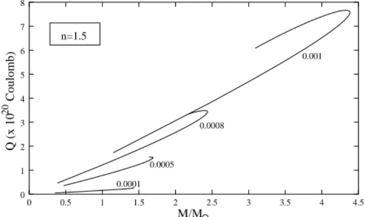
In Fig.(2) we plotted the mass-radius relation. Due to the effect of the repulsive force, the charged stars have large radius and larger mass as we should expect. Even if the radius is increasing with the mass, the M/R ratio is also in-creasing, but much slower. For the lower charge fractions, this increase in the radius is very small, but a look at the structure for the fractionf = 0.001reveals that for a mass of 4.3 M⊙, the radius goes as high as 35 kms. Though
the compactness of the stars are retained, they are now better to be called as charged compact starsrather than charged neutron stars. The charge fraction in the limit-ing case of maximally allowed value goes uptof = 0.0011, for which the maximum mass stable star forms at a lower central density even smaller than the nuclear matter den-sity. This extreme case is not shown in Fig.(2) because the radius of the star and its mass is very high (68 km & 9.7 M⊙ respectively) which suppresses the curves of the lower charge fractions due to scaling. For this star, the mass con-tribution from the electric energy density is 10% than that from the mass density. It can be checked by using relation (11) that this charge fraction f = 0.0011 corresponds to ρch= 0.95616×ρin geometrical units.
M/M
Q (x 10 Coulomb)
20
n=1.5
0.0001 0.0005
0.0008
0.001
. .
0 1 2 3 4 5 6 7 8
0 0.5 1 1.5 2 2.5 3 3.5 4 4.5
Figure 3. The variation of the charge with mass for differentf.
The Q× M diagram of Fig.(3) shows the mass of the stars against their surface charge. We have made the charge density proportional to the energy density and so it was ex-pected that the charge, which is a volume integral of the charge density, will go in the same way as the mass, which is also a volume integral over the mass density. The slope of the curves comes from the different charge fractions.The na-ture of the curves in fact reflects that charge varies with mass (with the turning back of the curves all falling in the ‘unsta-ble zone’ and is not taken into consideration). If we consider that the maximum allowed charge estimated by the condi-tion (U ≃√8πP <√8πǫ) for dP
dr to be negative (Eq. (8)), we see that the curve for the maximum charge in Fig.(3) has a slope of 1:1 (in a charge scale of 1020Coulombs1).
This scale can easily be understood if we write the charge as Q =√GM⊙ M
M⊙ ≃ 10
20 M
M⊙Coulombs.This charge Q is the charge at the surface of the star where the pressure and alsodPdr are zero. So, at the surface, the Coulomb force is es-sentially balanced by the gravitational force and the relation of the charge and mass distribution we found is exactly the same for the case of charged dust sphere discussed earlier by Papapetrou[7] and Bonnor[8].
The total mass of the systemMtot increases with
in-creasing charge because the electric energy densityadds on to the mass energy density. This change in the mass is low for smaller charge fraction and going upto 7 times the value of chargeless case for maximum allowed charge fraction
1
As electric energy density and pressure needs to be of the same order, so from the fine structure constantα=e~2c= 1
137,we get a relation for the charge and MeV/fm3
f = 0.0011. The most effective term in Eq.(8) is the fac-tor (Mtot+ 4πr3P∗). P∗ = P− U
2
8π is the effective pres-sure of the system because the effect of charge decreases the outward fluid pressure, negative in sign to the inward grav-itational pressure. With the increase of charge, the value of P∗ decreases, and hence the gravitational negative part of Eq.(8) decreases. So, with the softening of the pressure gradient, the system allows more radius for the star until it reaches the surface where the pressure (and dPdr) goes to zero. We should stress that because U8π2 cannot be too much larger than the pressure in order to maintain dPdr negative as discussed before, so we have a limit on the charge, which comes from the relativistic effects of the gravitational force and not just only from the repulsive Coulombian part.
Radius [kms]
dP5 dP8
dPc5 dPc8
dPg5 dPg8
.
.
n=1.5
−40 −35 −30 −25 −20 −15 −10 −5 0 5 10
0 2 4 6 8 10 12 14 16 18 20
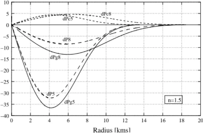
Figure 4. The positive Coulomb part and the gravitational nega-tive part of the pressure gradient together with the total (dPdr) are shown here for two different values of the charge factorf. For
f = 0.0005and 0.0008 coming from thematter partare
de-noted as dPg5 and dPg8 respectively, those fromCoulomb part
are dPc5 and dPc8 respectively. The corresponding totals are dP5 and dP8.
This effect is shown in Fig.(4) where we have plotted both the positive Coulomb part and the negative matter part of the pressure gradient. The plots are for two values of the charge fractionf = 0.0005andf = 0.0008. The positive part of dPdr maintains its almost constant value because the charge fractionf is the controller of the same, and in our case, they differ by a very small percentage. In the negative part, the changes are drastic and are mainly brought by the effective pressure as we already discussed.
In our high density system, the gravitational and the Coulomb forces are highly coupled. Although it is difficult to disentangle the forces, but to a common belief, it can be considered that the charged particles, due to their self cre-ated huge field, will leave the star very soon. This process will however lead to an imbalance of the global forces acting on the star, which were previously balanced by the Gravita-tional and the Coulomb forces. This process will help in the star to further collapse to a charged black hole. We say it charged because, by the time the system collapses, all the charge has not left the star, and they get trapped inside the black hole [17].
4
Conclusions
In our study, we have shown that a high density system like a neutron star can hold huge charge of the order of 1020 Coulomb considering the global balance of forces. With the increase of charge, the maximum mass of the star recedes back to a lower density regime. The stellar mass also in-creases rapidly in the critical limit of the maximum charge content, the systems can hold. The radius also increases ac-cordingly, however keeping the M/R ratio increasing with charge. The increase in mass is primarily brought in by the softening of the pressure gradient due to the presence of a Coulombian term coupled with the Gravitational matter part. Another intrinsic increase in the mass term comes through the addition of the electric energy density to the mass den-sity of the system.
The inside electric field of the charged stars are very high and crosses the critical field limit for pair creation (Beken-stein [5]). However, this issue is debatable because the crit-ical field has been calculated for vacuum and one does not really know what the value will be in a high density system. The stability of the charged stars are however ruled out from the consideration of forces acting on individual charged par-ticles. They face enormous radial repulsive force and leave the star in a very short time. This creates an imbalance of forces and the gravitational force overwhelms the repulsive Coulomb and fluid pressure forces and the star collapses to a charged black hole.
Finally, these charged stars are supposed to be very short lived, and are the intermediate state between a supernova collapse and charged black holes.
SR acknowledges the FAPERJ for research support, MM for the partial CNPQ support, and JSPL and VTZ for the hospitality of Observat´orio Nacional, Rio de Janeiro.
References
[1] S. Rosseland, Mont. Not. Royal Astronomical Society, 84, 720 (1924).
[2] A.S. Eddington, Internal Constitution of the stars, Cam-bridge University Press, CamCam-bridge, England, 1926.
[3] J. Bally and E.R. Harrison, ApJ 220, 743 (1978).
[4] N.K. Glendenning, Compact Stars: Nuclear Physics,
Parti-cle Physics, and General Relativity, Springer-Verlag (2000).
[5] J.D. Bekenstein, Phys. Rev. D4, 2185 (1971).
[6] S.D. Majumdar, Phys. Rev. D 72, 390 (1947).
[7] A. Papapetrou, Proc. R. Irish Acad. 81, 191 (1947).
[8] W.B. Bonnor and S.B.P. Wickramasuriya, Mon. Not. R. Astr. Soc. 170, 643 (1975).
[9] B.V. Ivanov (2002c), Phys. Rev. D. 65, 104001 (2002).
[10] J.L. Zhang, W.Y. Chau, and T.Y. Deng, Astrophys. & Space Sc. 88, 81 (1982).
[11] F. de Felice, Y. Yu, and Z. Fang, Mon. Not. R. Astron. Soc.
277 L17 (1995).
[13] F. de Felice, S.M. Liu, and Y.Q. Yu, Class. Quantum Grav.
16, 2669 (1999).
[14] P. Anninos and T. Rothman, Phys. Rev. D65, 024003 (2001).
[15] H.J. Mosquera Ceusta, A. Penna-Firme, and A. P´erez-Lorenzana, Phys. Rev. D 65, 087702 (2003).
[16] A.R. Taurines, C.A. Vasconcellos, M. Malheiro, and M. Chiapparini, Phys. Rev. C63, 065801 (2001).