Typical types and formation mechanisms of haze in an eastern Asia megacity, Shanghai

(1)

ACPD

11, 21713–21767, 2011

Typical types and formation mechanisms of haze

K. Huang et al.

Title Page

Abstract Introduction

Conclusions References

Tables Figures

◭ ◮

Back Close

Full Screen / Esc

Printer-friendly Version Interactive Discussion

Discussion

P

a

per

|

Dis

cussion

P

a

per

|

Discussion

P

a

per

|

Discussio

n

P

a

per

|

Atmos. Chem. Phys. Discuss., 11, 21713–21767, 2011 www.atmos-chem-phys-discuss.net/11/21713/2011/ doi:10.5194/acpd-11-21713-2011

Atmospheric Chemistry and Physics Discussions

This discussion paper is/has been under review for the journal Atmospheric Chemistry and Physics (ACP). Please refer to the corresponding final paper in ACP if available.

Typical types and formation mechanisms

of haze in an eastern Asia megacity,

Shanghai

K. Huang1,2, G. Zhuang1, Y. Lin1, J. S. Fu2, Q. Wang1, T. Liu1, R. Zhang1, Y. Jiang1, and C. Deng1

1

Center for Atmospheric Chemistry Study, Department of Environmental Science and Engineering, Fudan University, Shanghai, 200433, China

2

Department of Civil and Environmental Engineering, The University of Tennessee, Knoxville, TN 37996, USA

Received: 13 July 2011 – Accepted: 21 July 2011 – Published: 2 August 2011

Correspondence to: G. Zhuang (gzhuang@fudan.edu.cn), J. S. Fu (jsfu@utk.edu)

(2)

ACPD

11, 21713–21767, 2011

K. Huang et al.

Title Page

Tables Figures

◭ ◮

Back Close

Full Screen / Esc

Discussion

P

a

per

|

Dis

cussion

P

a

per

|

Discussion

P

a

per

|

Discussio

n

P

a

per

|

Abstract

An intensive aerosol and gases campaign has been performed at Shanghai in the Yangtze River Delta region over Eastern China from late March to early June 2009. This study provided a complementary picture of typical haze types and formation mecha-nisms in megacities over China by using a synergy of ground-based monitoring,

satel-5

lite observation and lidar inversion. During the whole study period, several extreme low visibility periods were observed with distinct characteristics, and three typical haze types were identified, i.e. secondary inorganic pollution, dust, and biomass burning. Sulfate, nitrate and ammonium accounted for a major part of PM₂_.₅ mass during the secondary inorganic pollution, and the good correlation between SO₂/NO_x/CO and

10

PM₂_.₅indicated that coal burning and vehicle emission were the major sources. Large-scale regions with high AOD and low ˚Angstr ¨om exponent were detected by remote-sensing observation during the dust pollution episode, and this episode corresponded to coarse particles rich in mineral components such as Al and Ca with mineral aerosol contributing 76.8 % to TSP. The relatively low Ca/Al ratio of 0.75 combined with the air

15

mass backward trajectory analysis suggested the dust source from Gobi Desert. Typi-cal tracers for biomass burning from satellite observation (column CO and HCHO) and from ground measurement (CO, particulate K+, OC, and EC) were greatly enhanced during the biomass burning pollution episode. The exclusive linear correlation between CO and PM₂_.₅ corroborated that organic aerosol dominated aerosol chemistry during

20

biomass burning, and the high concentration and enrichment degree of arsenic (As) could be also partly derived from biomass burning. Aerosol optical profile observed by lidar demonstrated that aerosol was mainly constrained below the boundary layer and comprised of spheric aerosol (depolarization ratio<5 %) during the secondary in-organic and biomass burning episodes, while during the dust episode thick dust layer

25

(3)

ACPD

11, 21713–21767, 2011

K. Huang et al.

Title Page

Tables Figures

◭ ◮

Back Close

Full Screen / Esc

Discussion

P

a

per

|

Dis

cussion

P

a

per

|

Discussion

P

a

per

|

Discussio

n

P

a

per

|

that identification of the complicated emission sources was important for the air quality improvement in megacities in China.

1 Introduction

China is now undergoing tremendous challenges of air quality impairment due to rapid industrial and transportation expansion, sharply increased demands of fossil fuel usage

5

and increasing populations. Primary pollutant concentrations grow as a power-law function of population, and in China large emissions were concentrated in the mega-city clusters, such as Jing-Jin-Ji (Beijing-Tianjin-Hebei), the Pearl River Delta and Yangtze River Delta (YRD) regions (Parrish and Zhu, 2009). The YRD region, on which this study was focusing, included the biggest city in China, Shanghai, and Jiangsu and

10

Zhejiang provinces. It has a population of over 80 million people and occupied over 21 % of China’s total gross domestic product (GDP).

Upon a globally decreasing trend of radiation, sunshine duration and sky visibility (Che et al., 2005; Kaiser and Qian, 2002; Wang et al., 2009), the YRD region had ex-perienced substantially increasing haze days since 1990s (Chang et al., 2009; Che et

15

al., 2007), which was attributed to the dimming effect of aerosol. Compared to Bejing and Guangzhou, the emissions of black carbon and NO_xin Shanghai were 2∼3 times

higher (2003_∼2005) (Chan and Yao, 2008), and the emission of NO_xwas predicted to increase 60–70 % by 2020 due to the expansion of transportation (Chen et al., 2006). Health effects, such as cardiorespiratory diseases and carcinogenesis were partially

20

associated with air pollution (Kan et al., 2007; Ye et al., 2000; Zhao et al., 2003) and reductions of primary PM₂_.₅ from industrial sector and mobile sources showed good health benefits in YRD (Zhou et al., 2010). It was estimated that the total economic cost of health impacts due to particulate air pollution in urban areas of Shanghai in 2001 was approximately 625.40 million US dollars, accounting for 1.03 % of GDP of

25

(4)

ACPD

11, 21713–21767, 2011

K. Huang et al.

Title Page

Tables Figures

◭ ◮

Back Close

Full Screen / Esc

Discussion

P

a

per

|

Dis

cussion

P

a

per

|

Discussion

P

a

per

|

Discussio

n

P

a

per

|

quality research had been conducted in Shanghai and other areas in YRD. Investiga-tion of major aerosol constituents were found to be sulfate, nitrate, ammonium (Wang et al., 2006; Yao et al., 2002; Ye et al., 2003) and organic aerosol (Feng et al., 2006; Feng et al., 2009; Yang et al., 2005a), concluding that fossil fuel combustion and ve-hicle emission were major sources of secondary components. Compared to Beijing,

5

Shanghai had higher concentrations of black carbon (BC) and higher ratio of BC/CO, which were attributed to larger contribution from diesel burning (diesel powered ve-hicles and marine vessels) (Zhou et al., 2009). Ground based sunphotometer ob-servation at various sites in YRD showed relatively high aerosol extinction to sunlight (AOD>0.7) and high fraction of fine particles ( ˚Angstr ¨om exponent>1.0) (Pan et al.,

10

2010; Xia et al., 2007). Concentration and fraction of ultrafine (10–100 nm) particles in total particle counts at Taichang, YRD, were 2∼3 times higher than those reported in

the urban/suburban areas in North America and Europe (Gao et al., 2009). And one research on the background site Lin’an suggested that the aerosol properties were more close to urban areas rather than the suburban ones (Xu et al., 2002). Huang et

15

al. (2008) found that there was a significantly decreasing trend of acid rain pH in Shang-hai with 15-fold increased acidity during 1997–2005. However, the mechanism on the formation of haze was seldom discussed (Fu et al., 2008; Pathak et al., 2009; Zhou et al., 2009). Compared to some intensive field campaigns in the Pearl River Delta region and northeastern China, i.e. PRIDE-PRD2004, PRIDE-PRD2006 (Program of

20

Regional Integrated Experiments on Air Quality over Pearl River Delta of China 2004 and 2006; Garland et al., 2008; Zhang et al., 2008), CAREBEIJING (Regional for-mation processes and controlling effects of air pollution before and during the Beijing Olympics: the results of CAREBEIJING; Wang et al., 2010), and EAST-AIRE (East Asian Studies of Tropospheric Aerosols: an International Regional Experiment; Li et

25

(5)

ACPD

11, 21713–21767, 2011

K. Huang et al.

Title Page

Tables Figures

◭ ◮

Back Close

Full Screen / Esc

Discussion

P

a

per

|

Dis

cussion

P

a

per

|

Discussion

P

a

per

|

Discussio

n

P

a

per

|

In this study, an intensive field experiment using various techniques was targeted to determine the typical pollution types that caused the frequent occurrence of haze in Eastern China. Aerosol chemical and optical experiments were combined with remote-sensing observation to distinguish and characterize different types of haze. Comments and discussions were made to emphasize the importance of aerosol source

determina-5

tion, which were beneficial for the local governments to improve air quality and mitigate climate effects.

2 Methodology

2.1 Field observations

2.1.1 Automatic aerosol and gases monitoring

10

The Thermo Scientific TEOM 1405-D monitor simultaneously measured PM₂_.₅, PM-Coarse (PM₁₀₋₂_.₅) and PM₁₀ mass concentration upon an oscillating balance. PM (particulate matter) accumulating on a filter mounted changes in the frequency of os-cillation, which were related to the mass of material accumulating on the filter, were detected in quasi-real-time and converted by a microprocessor into an equivalent PM

15

mass concentration every few seconds, as a 10 min running average. Sampler split a PM₁₀ sample stream into its fine (PM₂_.₅) and coarse (PM₁₀₋₂_.₅) fractions using a USEPA-designed virtual impactor for the additional 2.5 µm cutpoint. The total flow rate operated at 16.67 l min−1_{, and two separate flow controllers maintained the coarse}

par-ticle stream at 1.67 l min−1and the fine particle stream at 3.0 l min−1. Besides, another

20

Thermo Scientific TEOM 1405 monitor was set up to measure PM₁ mass concentra-tion operating at 3.0 l min−1_{with a bypass flow rate of 13.67 l min}−1_{. PM concentrations}

were averaged and used at intervals of 1hr in this study. Trace gases instruments included 43i SO₂ analyzer, 42i NO-NO₂-NO_x analyzer, 49i O₃ analyzer and 48i CO analyzer, zero and span checks were performed every week, all the data were also

25

(6)

ACPD

11, 21713–21767, 2011

K. Huang et al.

Title Page

Tables Figures

◭ ◮

Back Close

Full Screen / Esc

Discussion

P

a

per

|

Dis

cussion

P

a

per

|

Discussion

P

a

per

|

Discussio

n

P

a

per

|

2.1.2 Manual sampling

Aerosol samples of TSP and PM₂_.₅were collected on Whatman®41 filters (Whatman Inc., Maidstone, UK) using medium-volume samplers manufactured by Beijing Geolog-ical Instrument-Dickel Co., Ltd. (model: TSP/PM₁₀/PM₂_.₅–2; flow rate: 77.59 l min−1_).

Aerosol samples of PM₁₀ were collected on Whatman quartz microfiber filters (QM/A,

5

18.5 cm×23.7 cm) using the high-volume sampler (Thermo, flow rate: 1.00 m3min−1).

All the samplers were co-located with the online instruments on the roof (∼30 m) of the

4th Teaching Building at Fudan University, Shanghai. The duration time of sampling was generally 24 h. More samples with shorter duration time were collected during the heavy haze days. The filters before and after sampling were weighed using an

analyti-10

cal balance (Model: Sartorius 2004MP) with a reading precision 10 mg after stabilizing in constant temperature (20±1◦C) and humidity (40±1 %). All the procedures were

strictly quality controlled to avoid the possible contamination of samples.

2.1.3 Lidar observation

A dual-wavelength depolarization lidar (Model: L2S-SM II) developed by the National

15

Institute for Environmental Studies (NIES) was operated in this field campaign. The lidar could measure backscattering coefficients and the depolarization ratio at wave-length of 532 nm. The Lidar employed a flash lamp pumped Nd:YAG laser with a second harmonics generator. The laser beam was vertically oriented to the sky after collimated with a beam expander. Transmitted laser energy was typically 20 mJ per

20

pulse at 1064 nm and 30 mJ per pulse at 532 nm. The pulse repetition rate was 10 Hz. The scattered light was received with a 20 cm Schmidt Cassegrain type telescope colli-mated and directed to the dichroic mirror. The polarization components were detected with two photomultiplier tubes (PMTs). Detected signals were recorded with a transient recorder (digital oscilloscope), averaged and transferred to the data acquisition

com-25

(7)

ACPD

11, 21713–21767, 2011

K. Huang et al.

Title Page

Tables Figures

◭ ◮

Back Close

Full Screen / Esc

Discussion

P

a

per

|

Dis

cussion

P

a

per

|

Discussion

P

a

per

|

Discussio

n

P

a

per

|

method (Fernald, 1984) was applied to deriving the extinction coefficient with lidar ratio (extinction-to-backscatter ratio) set to 50 sr (Liu et al., 2002) in inversion process.

2.2 Chemical analysis

2.2.1 Ion analysis

One-fourth of each sample and blank filter was extracted ultrasonically by 10 ml

deion-5

ized water (18MΩcm−1). Eleven inorganic ions (SO2₄−, NO−₃, F−, Cl−, NO−₂, PO3₄−, NH+₄, Na+, K+, Ca2+, Mg2+) and four organic acids (formic, acetic, oxalic, and methyl-sulfonic acid (MSA)) were analyzed by Ion Chromatography (ICS 3000, Dionex), which consisted of a separation column (Dionex Ionpac AS 11), a guard column (Dionex Ionpac AG 11), a self-regenerating suppressed conductivity detector (Dionex Ionpac

10

ED50) and a gradient pump (Dionex Ionpac GP50). The detail procedures were given elsewhere (Yuan et al., 2003).

2.2.2 Element analysis

Half of each sample and blank filter was digested at 170◦_{C for 4 h in high-pressure}

Teflon digestion vessel with 3ml concentrated HNO₃, 1 ml concentrated HCl, and 1ml

15

concentrated HF. After cooling, the solutions were dried, and then diluted to 10 ml with distilled deionized water. Total 24 elements (Al, Fe, Mn, Mg, Mo, Ti, Sc, Na, Ba, Sr, Sb, Ca, Co, Ni, Cu, Ge, Pb, P, K, Zn, Cd, V, S, and As) were measured by using an inductively coupled plasma atomic emission spectroscopy (ICP-OES; SPECTRO, Germany). The detailed analytical procedures were given elsewhere (Sun et al., 2004;

20

Zhuang et al., 2001).

2.2.3 Carbonaceous aerosol analysis

(8)

ACPD

11, 21713–21767, 2011

K. Huang et al.

Title Page

Tables Figures

◭ ◮

Back Close

Full Screen / Esc

Discussion

P

a

per

|

Dis

cussion

P

a

per

|

Discussion

P

a

per

|

Discussio

n

P

a

per

|

IMPROVE thermal/optical reflectance (TOR) protocol (Chow and Watson, 2002) was used for the carbon analysis. The eight fractions (OC1, OC2, OC3, OC4 at 120, 250, 450 and 550◦C, respectively in a helium atmosphere, EC1, EC2, EC3 at 550, 700 and 800◦C, respectively, in the 98 % helium/2 % oxygen atmosphere) and OPC (optically detected pyrolized carbon) were measured separately. The IMPROVE protocol defined

5

OC as OC1+OC2+OC3+OC4+OPC and EC as EC1+EC2+EC3-OPC.

2.3 Satellite observation

In this study, a number of satellite sensors had been used to sense aerosol and trace gas information. The MODIS instrument (Moderate-resolution Imaging Spec-troradiometer) provided a large regional view of aerosol distributions with a resolution

10

of 10×10 km. Operational aerosol optical depths were reported at 0.55 µm by NASA

(Chu et al., 2003; Kaufman et al., 1997). The total carbon monoxide column concen-tration retrieved from Atmospheric Infrared Sounder (AIRS) on board NASA’s Aqua satellite were used to observe large scale transport from biomass burning sources (McMillan et al., 2005). Launched in 2004, the Dutch–Finnish built Ozone Monitoring

15

Instrument (OMI) aboard NASA’s EOS Aura satellite provided daily global coverage with a spatial resolution of 13 km×24 km at nadir (Levelt et al., 2006), and the

to-tal formaldehyde column concentration had been used to study the signals of possible biomass burning source. Detailed description about the OMI instrument could be found elsewhere (Kurosu et al., 2004).

20

3 Results and discussion

3.1 Identification of three pollution episodes

An intensive aerosol characterization campaign was carried out in Shanghai over the Yangtze River Delta region in 2009, which aimed to get insights into the forma-tion mechanisms of haze in Eastern China. The study period had a coverage of

25

(9)

ACPD

11, 21713–21767, 2011

K. Huang et al.

Title Page

Tables Figures

◭ ◮

Back Close

Full Screen / Esc

Discussion

P

a

per

|

Dis

cussion

P

a

per

|

Discussion

P

a

per

|

Discussio

n

P

a

per

|

time periods were due to malfunction and maintenance of some instruments. Haze was usually defined as an atmospheric phenomenon where dust, smoke and other pollutant particles reduced the visibility of the sky. Here we had calculated the visibility follow-ing the Koschmieder formulaL_V=3.912/σ_ext, whereL_V was the visibility and the total extinction coefficientσ_extwas due to scattering and absorption by particles and gases.

5

In order to compare with the recorded visibility data, we calculated the near-surface extinction coefficient caused by aerosol (σ_ep) by averaging the lidar measured aerosol extinction coefficient from the ground to an altitude of 300 m. Absorption of visible light by gases was considered to be essentially due to NO₂ and the absorption coef-ficient (σ_ag) could be estimated using the formula σ_ag =0.33×[NO2] (Groblicki et al.,

10

1981). Here, NO₂ was in units of ×10−9V/V. Rayleigh scattering coefficient (σsg) was

assumed to be a constant of 0.013 km−1_{a.s.l. (Chan et al., 1999; Peundorf, 1957). The}

scattering coefficient of light due to moisture in the air (b_sw) could be neglected when relatively humidity (RH) was lower than 70 % (Cass, 1979; Chan et al., 1999). In this study, the average relative humidity was about 60 %. Consequently, the total light

ex-15

tinction by particles and gases (σ_ext=σ_ep+σ_ag+σ_sg) was calculated and the visibility could be estimated. Figure 1a shows the calculated hourly visibility and the recorded visibility at Pudong, which was about 32 km from the site in this study (An upper limit of L_V=10 km was recorded at the meteorological station of Pudong). As shown in the fig-ure, the visibility measured by two different approaches had relatively good time-series

20

consistency, especially during the low visibility periods, which suggested that visibilities estimated from aerosol extinction profile and pollutant gas were reasonable and could be used for further analysis.

Figure 1b shows the temporal variation of PM mass concentration levels at three dif-ferent sizes, i.e. PM₁, PM₂_.₅and PM₁₀. Based on the visibility, PM mass concentration

25

(10)

ACPD

11, 21713–21767, 2011

K. Huang et al.

Title Page

Tables Figures

◭ ◮

Back Close

Full Screen / Esc

Discussion

P

a

per

|

Dis

cussion

P

a

per

|

Discussion

P

a

per

|

Discussio

n

P

a

per

|

If we applied the US EPA 24-h standard of 35 µg m−3_{, the fine particle}

concentra-tion levels were much higher than this criteria. The average ratio of PM₂_.₅/PM₁₀ was 0.54±0.09, indicating both fine and coarse particles could be important in the

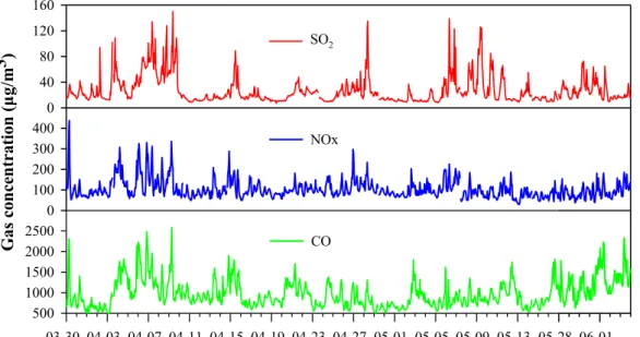
forma-tion of polluforma-tion. The mass ratio of PM₁/PM₂_.₅ ranged from 0.90 to 0.99, indicating particles tended to accumulated in smaller sizes. Time series of pollutant gases, i.e.

5

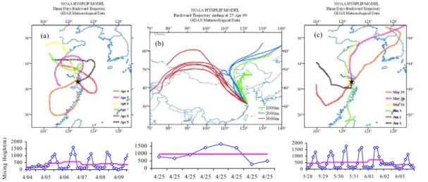
SO₂, NO_x and CO, showed their significant enhancements during this period (Fig. 2), enhanced industrial and tra_ffic emissions were probably responsible for this and the pollution during this period was probably caused by the local photochemical pro-cess. The detailed analysis on pollutant gases would be discussed in Sect. 3.5. To study the aerosol transport characteristics, air mass backward trajectories were

com-10

puted using the NOAA Hybrid Single-Particle Lagrangian Trajectory (HYSPLIT) model (R. Draxler and G. Rolph, HYSPLIT (HYbrid Single–Particle Lagrangian Integrated Tra-jectory) Model, 2003, http://www.arl.noaa.gov/ready/hysplit4.html) with meteorological data provided by the Global Data Assimilation System (GDAS). Three-day backward trajectories at the end point of Shanghai during PE1 showed that air masses flowed

15

from various directions and traveled relatively short distances, reflecting the slow wind speeds. Additionally, the daily average mixing layer was almost below 500 m (Fig. 3a). This typical stagnant synoptic meteorological condition was especially unfavorable for the dispersion of particles and gases, and beneficial for the formation of haze pollution. The second pollution episode (PE2) occurred on 25 April and lasted a short duration.

20

The daily concentrations of PM₁, PM₂_.₅, and PM₁₀ were 26.3, 53.0, and 174.5 µg m−3_,

respectively. And the ratio of PM₂_.₅/PM₁₀ reached the lowest value of 0.35 over the whole study period, indicating the characteristic of coarse particle pollution. Combined with air backward trajectory analysis, we found that air masses starting at various al-titudes of 500, 1000 and 3000 mall flowed from northern China, which passed over

25

(11)

ACPD

11, 21713–21767, 2011

K. Huang et al.

Title Page

Tables Figures

◭ ◮

Back Close

Full Screen / Esc

Discussion

P

a

per

|

Dis

cussion

P

a

per

|

Discussion

P

a

per

|

Discussio

n

P

a

per

|

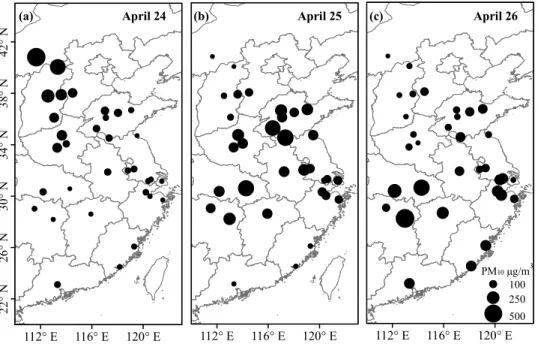
probably caused by the entrainment of dust aerosol from the desert in Mongolia and Inner-Mongolia via the long-range transport. Figure 4 depicts the regional distribution pattern of PM₁₀ concentration during 24–26 April in northern and eastern China. On 24 April, high pollution (PM₁₀>300 µg m−3) occurred in the northern China, mainly in Inner-Mongolia and Shanxi province while the eastern and southern China was

virtu-5

ally dust-free (Fig. 4a). On the next day, high level particles moved to major areas of central China and stretched to the eastern coastal regions (Fig. 4b). As for Shanghai, our monitoring station observed that the dust entrainment actually had the most signif-icant impacts on local air quality during two periods, i.e. from 01:30 to 08:00 LST and 17:00 to 23:00 LST (Local Standard Time). The average PM₁₀ concentration reached

10

258 and 236 µg m−3_{, respectively, while the concentrations of fine particles and}

pollu-tant gases stayed at low levels (Figs. 1b and 2), which was due to the dilution effect of dust on local pollutants. Till 26 April, the PM levels in northern China had sharply declined and the dust continued to travel southwestward along the east coast, which exerted a moderate influence on air quality of southern China (Fig. 4c). In Shanghai,

15

there was a significant decrease of PM₁₀ concentration and an increase of PM₂_.₅/PM₁₀ ratio to over 0.50, indicating the re-dominance of fine particles after the pass of dust.

The third pollution episode (PE3) occurred from 28 May to 3 April. The av-erage concentrations of PM₁, PM₂_.₅, and PM₁₀ were 67.8±37.6, 84.0±48.4 and

135.6_±71.4 µg m−3_{, respectively, with the average PM}

2.5/PM10ratio of 0.65±0.04.

20

Fine particle concentration levels and its mass contribution to the total particles were both the highest among all three pollution episodes. Notwithstanding, the concentra-tion levels of pollutant gases were not as high as PE1 except for CO, SO₂ was at a moderate level and NO_x was relatively low (Fig. 2). Opposite to the high concentra-tions of pollutant gases during PE1, the formation mechanism of the PE3 pollution

25

(12)

ACPD

11, 21713–21767, 2011

K. Huang et al.

Title Page

Tables Figures

◭ ◮

Back Close

Full Screen / Esc

Discussion

P

a

per

|

Dis

cussion

P

a

per

|

Discussion

P

a

per

|

Discussio

n

P

a

per

|

However, it was still difficult to identify the pollution types of different episodes based on the limited information such as PM, pollutant gases and meteorological parameters. In the discussions below, we will demonstrate more evidences from the aerosol optical and chemical properties.

3.2 Regional characteristics and possible sources via remote sensing

5

observation

The remote sensing analysis from satellite observation is a good way to indicate the spatial distribution, transport and possible source of airborne pollutants. Figure 5 shows the observed satellite signals during the three episodes, respectively. During PE1, zones of high aerosol optical depths (AOD) at the wavelength of 550 nm

re-10

trieved from MODIS were mainly concentrated in Jing-Jin-Ji (Beijing-Tianjin-Hebei), Shandong, Anhui, Henan, Hubei provinves, and the Yangtze River Delta region, includ-ing northern part of Zhejiang, Jiangsu provinces and Shanghai (Fig. 5a). The average AOD value over Shanghai reached extremely high value of over 1.2, indicating strong aerosol extinction to sunlight in the atmosphere. Figure 5b shows the spatial

distri-15

bution of ˚Angstr öm exponent at the wavelength range from 470 to 670 nm. ˚Angstr öm exponent was a good indicator of the aerosol size distribution, the larger this parameter, the smaller the particle size, and vice versa. The spatial pattern of ˚Angstr öm exponent didn’t resemble that of AOD. In some regions that the AOD values were moderate such as southern parts of Zhejiang province and major parts of central China, the ˚Angstr öm

20

exponents ranged from 1.3 to 1.5, indicating these regions were mainly dominated by fine particles. While in the high AOD regions that discussed above, the ˚Angstr ¨om ex-ponents were not correspondingly high and ranged from 0.8 to 1.2, which suggested there was non-negligible contribution of coarse particles during PE1. This was consis-tent with the moderate PM₂_.₅/PM₁₀ ratio that measured by our ground monitoring as

25

(13)

ACPD

11, 21713–21767, 2011

K. Huang et al.

Title Page

Tables Figures

◭ ◮

Back Close

Full Screen / Esc

Discussion

P

a

per

|

Dis

cussion

P

a

per

|

Discussion

P

a

per

|

Discussio

n

P

a

per

|

River Delta region along the east coast. The continuity of ˚Angstr ¨om exponent probably indicated that the Yangtze River Delta could have been more or less influenced from the northern China. As PE1 was in the spring season when the occurrence of floating dust was frequent and ubiquitous, the downstream regions were probably influenced by the transport of dust aerosol to some extent.

5

During PE2, high AOD values were observed in most parts of the study domain, which was as similar as PE1 to a certain extent, especially in the central and eastern parts of China with AOD exceeding 1.2 (Fig. 5c). Anyway, ˚Angstr ¨om exponents were much lower than PE1. It ranged from 0.5 to 0.6 (Fig. 5d), indicating considerable existence of coarse particles, which was consistent with ground measurements. And

10

there were almost no regional gradients of the ˚Angstr ¨om exponents, suggesting this episode was characteristic of large-scale influences. In Sect. 3.1, we have proposed that this pollution episode should be impacted by the invaded dust, and it was confirmed here by using the remote sensing analysis.

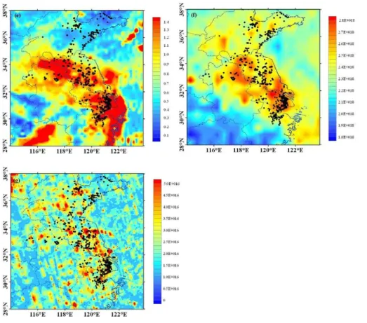
During PE3, large quantities of fire spots retrieved from MODIS were observed in

15

the study domain (denoted by black dots in Fig. 5e–g), and they were mainly located in the conjunction of western Shanghai and southern Jiangsu province, major parts of Jiangsu, northern Zhejiang, northern Anhui province and eastern parts of Shan-dong province. The total column concentration of carbon monoxide (CO) retrieved from the Atmospheric Infrared Sounder (AIRS) showed very good spatial pattern with

20

that of fire spots (Fig. 5e). In the normal times, the major sources of CO were derived from anthropogenic sources, such as traffic and/or industrial emission. While it was a major product emitted from biomass burning along with many trace gases such as car-bon dioxide (CO₂), methane (CH₄), nitrous oxides (NO_x) and hydrocarbons (Crutzen and Andreae, 1990). Various studies had used CO as tracer for biomass burning

25

(14)

ACPD

11, 21713–21767, 2011

K. Huang et al.

Title Page

Tables Figures

◭ ◮

Back Close

Full Screen / Esc

Discussion

P

a

per

|

Dis

cussion

P

a

per

|

Discussion

P

a

per

|

Discussio

n

P

a

per

|

areas free of biomass burning and close to the levels when biomass burning occurred in northeastern China (Choi and Chang, 2006). Besides, the Ozone Monitoring In-strument (OMI) also detected high formaldehyde (HCHO) columns over the intense burning areas (Fig. 5f). HCHO was a primary emission product from biomass burning, which was an intermediate product from the oxidation of hydrocarbons. And it was a

5

good indicator of the local photochemical source as it only had a lifetime of a few hours. HCHO columns over the hotspot regions were greater than 3.0×1016molecules cm−2,

more than a factor of 2–4 larger than the areas free of fires. Significant correlation be-tween HCHO columns and fire counts had ever been observed (Marbach et al., 2008; Palmer et al., 2007). Thus, the enhancement of CO and HCHO in the accumulated

10

fire spot regions indicated that the pollution during PE3 should be caused by biomass burning. The biomass emission resulted in high AOD values where large fire spots occurred, with the highest AOD up to about 2.0 in the Yangtze River Delta region. However, compared to the spatial distribution of CO and HCHO, the high AOD levels didn’t always coincide with the fire regions. For example, there was no fire spots

ob-15

served in Jiangxi province with low CO concentrations, but a high AOD region was found there. While as for Shandong province, the regions with great fire spots, high CO, and HCHO concentrations were at the relatively low AOD level. This suggested that CO and HCHO were more sensitive to biomass burning than AOD as AOD repre-sented the overall extinction of various emission sources to light rather than the single

20

source from biomass burning. The relatively low AOD over the Shandong Peninsula could have been due to the cleanup effect of the sea breezes as it was close to the sea. Anyway, the relatively good consistency between the observed satellite signals (e.g. carbon monoxide, formaldehyde and aerosol optical depth) over Eastern China and the fire hotspots clearly indicated that biomass burning should be the major cause

25

(15)

ACPD

11, 21713–21767, 2011

K. Huang et al.

Title Page

Tables Figures

◭ ◮

Back Close

Full Screen / Esc

Discussion

P

a

per

|

Dis

cussion

P

a

per

|

Discussion

P

a

per

|

Discussio

n

P

a

per

|

(Wang et al., 2002) and in autumn (Xu et al., 2002), which was due to the burning of post-harvest straws by human activities.

In this section, the remote sensing analysis had given us some highlights into the dif-ferent characteristics of three pollution episodes, including possible sources and trans-port pathways and provided some consistent results to our ground measurements.

5

However, there were large uncertainties due to satellite detection limit of the small fire size of the field crop residue burning that could be possibly missed by satellite obser-vations (Chang and Song, 2010; Yan et al., 2006). And satellites could not capture all fire events occurring during this study period, because fires hidden under clouds could not be easily detected. Additionally, satellite overpass also brings about the missed

10

detection of hotspots.

3.3 Aerosol chemistry under different atmospheric conditions

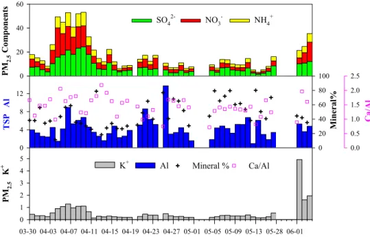
In order to further identify the di_fferent types of hazes as envisioned by the discussion above, we have demonstrated the results of aerosol chemical measurements here. Figure 6 shows the temporal variations of some typical aerosol components during the

15

whole study period. Time series of three major secondary inorganic species in PM₂_.₅, i.e. SO2₄−, NO−₃, and NH+₄ were presented in Fig. 6a. Obviously, the total concentra-tions of the three species above exhibited the highest levels during PE1 with average concentrations of 48.86_±5.01 µg m−3_{, which accounted an average of 77 % to PM}

2.5

mass. As precursors of sulfate and nitrate, SO₂and NO_xalso showed the highest levels

20

during this episode which had been stated in Sect. 3.1. This suggested that the pol-lution during PE1 was dominated by the secondary inorganic aerosol. In addition, we found that during EP3, these species also exhibited a moderate concentration level with average values of 27.12±7.37 µg m−3, which probably indicated that biomass burning

could also released considerable amounts of inorganic pollutants. For the other

peri-25

ods, the levels of theses species were much lower with values almost below 20 µg m−3. The average sulfate level during the whole study period was 8.0±5.8 µg m−3.

(16)

ACPD

11, 21713–21767, 2011

K. Huang et al.

Title Page

Tables Figures

◭ ◮

Back Close

Full Screen / Esc

Discussion

P

a

per

|

Dis

cussion

P

a

per

|

Discussion

P

a

per

|

Discussio

n

P

a

per

|

Yao et al., 2002; Ye et al., 2003), sulfate was much lower in this study, indicating the effective policy controls on the SO₂emission. However, the average nitrate concentra-tion reached 6.3_±5.7 µg m−3_{, comparable or even higher than those previous results.}

Additionally, the mass ratio of NO−₃/SO2₄− of 0.75±0.26 in this study had an increasing

trend as compared to the values of 0.64 in 2006 (Wang et al., 2006), and 0.43 during

5

1999–2000 (Yao et al., 2002; Ye et al., 2003). The ratio of NO−

3/SO

2−

4 could be used as

an indicator of the relative importance of stationary vs. mobile sources (Arimoto et al., 1996) and the results indicated that the role of mobile emission had become more and more significant due to the rapid expansion of transportation.

Figure 6b shows the temporal variation of elemental Al concentration, the ratio of

10

Ca/Al, and the estimated mass fraction of mineral aerosol in the total suspended par-ticles (TSP). Al was one of the inert and abundant elements in mineral aerosol and had been used as a good tracer for mineral aerosol in various studies (Huang et al., 2010; Wang et al., 2007; Zhang et al., 2010). As shown in the figure, the highest Al concentration occurred on 25 April, i.e, the second pollution episode (PE2). The

15

daily Al concentration reached as high as 13.7 µg m−3, almost 2∼3 times that of the

other periods. To quantify the mass concentration of mineral aerosol, it could be es-timated by summing the major mineral elements with oxygen for their normal oxides, which was calculated using the formula: [Mineral concentration]=2.2[Al] + 2.49[Si] + 1.63[Ca] + 2.42[Fe] + 1.94[Ti] (Malm et al., 1994). According to this estimation,

20

the percentage of mineral aerosol in TSP during PE2 was as high as 76.8 %. Op-positely, the average concentration of sum of SO2₄−, NO−₃, and NH+₄ in PM₂_.₅ was only 11.23±5.25 µg m−3, which was the lowest during the whole study period, indicating the

dominance of non-anthropogenic sources and the prominent impact of dust entrain-ment on the local aerosol chemistry. To further characterize the origin of dust, the

tem-25

(17)

ACPD

11, 21713–21767, 2011

K. Huang et al.

Title Page

Tables Figures

◭ ◮

Back Close

Full Screen / Esc

Discussion

P

a

per

|

Dis

cussion

P

a

per

|

Discussion

P

a

per

|

Discussio

n

P

a

per

|

relatively high Ca/Al ratios during the non-dust periods were attributed to the frequent construction activities in recent years in Shanghai (Wang et al., 2006). The signifi-cant drop of Ca/Al ratio during PE2 confirmed that the local air quality must have been impacted by the outside sources. Elemental ratios of Ca/Al of dust aerosol in the three major dust source regions of China, i.,e., Gobi Desert, Loess Plateau, and

Tak-5

limakan Desert, were 0.52±0.05, 1.09±0.13, and 1.56±0.14, respectively (Huang

et al., 2010). Combined with the backward trajectory analysis in Sect. 3.1, we could confirm that the aerosol chemistry over Shanghai during PE2 was more close to that of the dust aerosol originating from Gobi Desert.

Figure 6c shows the temporal variation of particulate K+ concentration in PM₂_.₅,

10

which was a good indicator for tracing the biomass burning source (Andreae, 1983). Its highest level occurred just during PE3, with the average concentration of 2.84 µg m−3, elevated 5∼10 times compared to the other days. As K+ could be also derived from

soil and dust, we used the K/Fe ratio of 0.56 (Yang et al., 2005b) to exclude the contri-bution of mineral source. It was calculated that the biomass burning derived K+ could

15

contribute about 80 % of total K+, indicating the significant influence of biomass burn-ing. The total potassium accounted for an average of 3.25 % in PM₂_.₅, also higher than that of 1.07 % in the other times and close to that of 3.58 % observed during the Mount Tai Experiment 2006 (MTX2006) which focused on biomass burning in East-ern China (Deng et al., 2011). Cl− _{and K}+ _{were both important ions in particles from} 20

open burning of agricultural wastes (Li et al., 2007a). In this study, a very high cor-relation between Cl− and K+ was observed with the correlation coefficient of 0.96. Individual particle analysis also found that large irregular shaped KCl particles existed in young smoke (Chakrabarty et al., 2006; Li et al., 2003). Another significantly en-hanced group of aerosol was the organic aerosol, including organic carbon (OC) and

25

element carbon (EC). OC and EC in PM₁₀ averaged 35.8±8.1 and 5.7±1.3 µg m−3

(18)

ACPD

11, 21713–21767, 2011

K. Huang et al.

Title Page

Tables Figures

◭ ◮

Back Close

Full Screen / Esc

Discussion

P

a

per

|

Dis

cussion

P

a

per

|

Discussion

P

a

per

|

Discussio

n

P

a

per

|

applied an OM/OC ratio of 1.8 to estimate the mass of organic matter (OM) (Turpin and Lim, 2001), the average mass contribution of OM to PM₁₀ would be as high as 50 %. However, a higher factor (2.2–2.6) for aerosol heavily impacted by smoke was recommended (Turpin and Lim, 2001), thus it may result in an underestimated value for the faction of OM in this work. Compared to previous results of the mass

percent-5

age of organic aerosol of∼30 % over YRD in the non-biomass-burning times (Feng et

al., 2009; Yang et al., 2005a), biomass burning evidently emitted much more hydrocar-bons. The OC/EC ratio was commonly on the order of 3 in most urban cities of China (Zhang et al., 2008), where the major sources of OC and EC were dominated by fossil fuel combustions. High ratio of OC/EC (6.4) was observed during PE3, which indicated

10

that biomass burning contributed far more organic carbon than fossil fuel combustion did (Yan et al., 2006). Field measurements also observed a high ratio of OC/EC (5) for the burning of wheat straw and an even higher ratio for maize stover (Li et al., 2007).

Figure 7 shows the enrichment factors (EF) of major elements in PM₂_.₅during three episodes, respectively, which aimed to evaluate the enrichment extents of various

el-15

ements in aerosol. Usually Al was used as the reference element as it was a rela-tively chemical inert element and almost had no anthropogenic sources. The calcula-tion formula was EF_x₌(X/Al)_aerosol/(X/Al)_crust, of whichX was the element of interest. Species with EFs less than 10 were usually considered to have a major natural source, which included Sc, Na, Ca, Co, Fe, Mn, Sr, Ba, P, K, Ni, Mn, Ti, and V. While species

20

with higher EFs were contaminated by anthropogenic sources, which included Cu, Mo, As, Sb, Ge, Pb, Zn, Cd, S, and Se. As shown in the figure, the enrichment degrees of almost all the elements were the lowest during PE2. The dust aerosol originating from the Gobi Desert was relatively clean (Huang et al., 2010), and its entrainment had a cleanup and dilution effect on the local pollution, which lowered the enrichment

25

(19)

ACPD

11, 21713–21767, 2011

K. Huang et al.

Title Page

Tables Figures

◭ ◮

Back Close

Full Screen / Esc

Discussion

P

a

per

|

Dis

cussion

P

a

per

|

Discussion

P

a

per

|

Discussio

n

P

a

per

|

1997 in Shanghai (Chen et al., 2005; Tan et al., 2006; Zhang et al., 2009). Zn and Cd mainly derived from local industrial and tra_ffic emission (Cao et al., 2008; Shi et al., 2008). As indicators for coal combustion (Nriagu, 1989), S and Se had the highest EFs among all the elements, indicating coal combustion was one of the major sources of air pollution in Shanghai. Most of the EFs of pollution elements during the biomass

5

burning period, i.e. PE3, were higher than PE2 and lower than PE1. The only excep-tion was arsenic (As), whose EF was comparable to that during PE1. The average As concentration during PE3 was 7.53 ng m−3_{, higher than that of 4.46 ng m}−3 _during

PE1 and much higher than 2.02 ng m−3 in the normal periods. The high concentration and great enrichment of As should not be derived from its usual source such as coal

10

burning, as no corresponding enrichment of the other pollution elements were found as in the PE1 case. High arsenic levels in groundwater in many areas over mainland China were observed (Mandal and Suzuki, 2002) and crop was most susceptible to As toxicity which sourced from the As-contaminated groundwater used for irrigation (Brammer and Ravenscroft, 2009). Thereby, the burning of agricultural residues would

15

probably release considerable amounts of As, which resulted in the enrichment of As in particles.

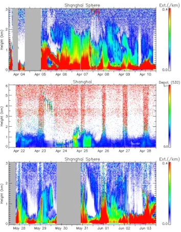
3.4 Aerosol vertical profile

Figure 8 shows the time-height cross-section of the lidar measured aerosol properties at the wavelength of 532 nm during the three pollution periods, respectively. In this

20

study, the total aerosol extinction coefficient was split to non-dust (spherical aerosols such as air pollution) and dust (nonspherical aerosol) fractions based on the aerosol depolarization ratio. Sugimoto et al. (2002) and Shimizu et al. (2004) described details of lidar observation and splitting method. Figure 8a presents the time-height cross-section of spheric aerosol extinction coe_fficient during PE1. Lidar observation

suc-25

(20)

ACPD

11, 21713–21767, 2011

K. Huang et al.

Title Page

Tables Figures

◭ ◮

Back Close

Full Screen / Esc

Discussion

P

a

per

|

Dis

cussion

P

a

per

|

Discussion

P

a

per

|

Discussio

n

P

a

per

|

layers, which reflected that pollutants were mainly constrained near the surface ground. The height of the boundary layer could be visually assumed from the vertical profile of aerosol optical properties. The profile, where the extinction coe_fficient sharply de-creased, could be determined as the top of planetary boundary layer (PBL) (Noh et al., 2007). During the daytime, the PBL height was relatively high, and sometimes it could

5

reach up to 2 km, which was due to the higher temperature and strong air convection. While during nighttime, it dropped to less than 0.5 km due to the temperature inversion. We selected one typical day (6 April) during PE1 to discuss its vertical profile (Fig. 9a). The depolarization ratio at the wavelength of 532 nm (δ₅₃₂) from the ground to the up-per layer (∼1.5 km) was less than 5 %, indicating the aerosol was mainly composed of 10

spheric particles. While at higher altitudes, the depolarization ratio increased a little bit, which could be due to the absence of spheric aerosol or the possible contamination of water clouds and ice clouds. The averaged profile of attenuated aerosol backscattering coefficient showed a steep decreased gradient from 0.037 km−1_sr−1 _{near the ground}

to 0.0018–0.0030 km−1_sr−1_{around 1–1.5 km.}

15

As for PE2, we presented the time-height cross section of depolarization ratio during 22–28 April (Fig. 8b). The depolarization ratio showed high values on 25 April. The high depolarization ratio of aerosol was due to the nonsphericity (irregular shapes) and relatively large size of particles (Mcneil and Carswell, 1975) and we regarded this type of aerosol as mineral aerosol/dust aerosol for that dust was the most important

com-20

ponent of nonspheric aerosols in East Asia. On 25 April, two consecutive dust plumes were observed, which was consistent with the ground measurement. We selected one dust plume (01:30–08:00 LST, 25 April) to discuss its vertical profile (Fig. 9b). In addition to the profile of aerosol backscattering coe_fficient and total depolarization ra-tio, the fraction of dust aerosol extinction to the total aerosol extinction (f_d) was also

25

(21)

ACPD

11, 21713–21767, 2011

K. Huang et al.

Title Page

Tables Figures

◭ ◮

Back Close

Full Screen / Esc

Discussion

P

a

per

|

Dis

cussion

P

a

per

|

Discussion

P

a

per

|

Discussio

n

P

a

per

|

the coe_fficient almost stayed constant value of about 0.01 km−1_sr−1 _{between 0.7 and}

1.0 km, which indicated the transport of outside aerosol and this phenomena hadn’t been observed in the other two episodes. Upwards, the backscattering coefficient started to sharply decrease again to low values. This type of vertical distribution of backscattering coefficient was closely related to the profile of depolarization ratio. As

5

shown in the figure, there was an increase ofδ₅₃₂ from ground and peaked at around 1.0 km with value of 0.155. Correspondingly, the contribution of dust aerosol extinction to the total aerosol extinction peaked between 0.7 and 1.0 km with the values ranging from 51 % to 57 %. Thus, the relatively constant backscattering coefficient between altitudes of 0.7 and 1.0 km should be due to the increase of dust aerosol. Above this

10

layer,f_dwas less than 10 %, indicating the negligible existence of nonspheric aerosol in the upper layers. Using a threshold ofδ532 =0.06 to distinguish dust from other types

of aerosol (Liu et al., 2008), the dust layer mainly distributed between ground and up to an altitude of around 1.4 km. The averageδ₅₃₂ value of this layer was 0.122±0.023,

which was close to the dust observed in Korea that sourced from the same dust region

15

(Kim et al., 2010). Above this layer, theδ₅₃₂ values decreased to low values, indicat-ing the transport of dust at relatively low altitudes. Actually, most of the dust plumes (approximately 70 %) were observed near the ground (Kim et al., 2010). The contribu-tion of dust aerosol extinccontribu-tion to the total aerosol extinccontribu-tion exhibited high values and relatively small vertical variations from near the ground to the upper layer of around

20

1 km, ranging from 44 % to 55 %. If we applied the dust and soluble aerosol extinction e_fficiency (σ_ep) of about 0.5 and 3 m2g−1_{, respectively (Lee et al., 2009), it could be}

estimated that the mass concentration of dust aerosol was almost 4∼7 times that of

spheric aerosol by using the formula,σep =βext/M, of whichβext andM represented

the extinction coe_fficient and mass concentration of dust/spheric aerosol. This was

25

consistent with our ground measurement that dust aerosol contributed 76.8 % to the total aerosol mass as discussed in Sect. 3.3.

(22)

ACPD

11, 21713–21767, 2011

K. Huang et al.

Title Page

Tables Figures

◭ ◮

Back Close

Full Screen / Esc

Discussion

P

a

per

|

Dis

cussion

P

a

per

|

Discussion

P

a

per

|

Discussio

n

P

a

per

|

temporal variations were observed. Compared to PE3, the PBL height during this pe-riod was even lower. Figure 9c shows the vertical profile of backscattering coe_fficient and depolarization ratio on 1 June. The depolarization ratio fluctuated within 0.05 in the whole layer, indicating the dominance of spheric particles. The backscattering co-e_fficient was about 0.024 km−1_sr−1_{near the surface, much lower than PE1 and PE2.} 5

While the fine aerosol concentration during PE3 was the highest. The non-linearity be-tween PM concentrations and optical properties should be due to the different chemical compositions among di_fferent periods. In biomass burning, organic aerosol dominated while sulfate ammonium, nitrate ammonium dominated during the secondary inorganic pollution episode. The mass scattering efficiency (m2g−1) of organics was about a

fac-10

tor of 2∼3 lower than that of sulfate (Hasan and Dzubay, 1983; Ouimette and Flagan,

1982), thus this discrepancy resulted in the non-linearity between PM concentrations and optical properties.

3.5 Trace gases

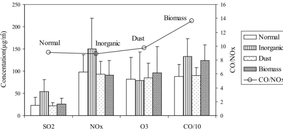
Figure 10 compares the concentrations of trace gases among three pollution episodes

15

and the normal period. The normal period was defined as the remaining days exclud-ing the three pollution episodes. O₃ during PE1 was the lowest with average concen-tration of 79_±63 µg m−3_{, and O}

3 and NOx were strongly anti-correlated, which was

due to the titration effect of nitrogen oxides as the Yangtze River Delta was under a strong VOC-limited regime (Geng et al., 2009). O₃ was highest during PE3 with

av-20

erage concentration of 96_±63 µg m−3_{, which could be caused by the relatively high}

emission of hydrocarbons emitted from biomass burning and the relatively weak titra-tion effect due to NO_x. During PE1, the average concentrations of SO₂, NO_x and CO reached 54, 150, and 1334 µg m−3_{, respectively. Compared to the heaviest}

pol-lution recorded at Shanghai on 19 January in 2007, when the daily concentration of

25

(23)

ACPD

11, 21713–21767, 2011

K. Huang et al.

Title Page

Tables Figures

◭ ◮

Back Close

Full Screen / Esc

Discussion

P

a

per

|

Dis

cussion

P

a

per

|

Discussion

P

a

per

|

Discussio

n

P

a

per

|

policies in China that mitigated the SO₂ emission, including desulfurization of coal-fired power plant plumes, decommissioning of coal-coal-fired boilers in manufacturing facil-ities and small power plants, conversion of domestic coal use to cleaner fuels and etc. (Fang et al., 2009). The emission of SO₂almost remained constant during 1996–2005 (Chan and Yao, 2008) and energy policy scenarios claimed that SO₂emissions during

5

2000–2020 would maintain the same level as in 2000 (Chen et al., 2006). The prob-lem for the present and future would be nitrogen oxides. The average concentration of NO₂and NO_x during PE1 reached high levels of 109 and 150 µg m−3_{, respectively.}

Even during the normal period, their concentration was 60 and 99 µg m−3_{, respectively,}

contrasting to 3–40 ppbv NO_x(1ppbv NO_xequaled to about 1.9 µg m−3) in 2007 (Geng

10

et al., 2009) and 5–35 µg m−3 NO_x in 1999 (Wang et al., 2003). Satellite observation and model simulation both detected and predicted a strong increase of NO₂in Eastern China, especially after 2000 (He et al., 2007), and Shanghai had a significantly linear increase of NO₂ column concentrations with about 20 % per year during the period of 1996–2005 (van der A et al., 2006), which was the rapidest among all the

mega-15

cities in China (Zhang et al., 2007). Due to the expansion of transportation system, NO_x emissions were projected to increase by 60–70 % by 2020 (Chen et al., 2006). Therefore, it could explain the relatively high concentration of particulate nitrate and increasing ratio of SO2₄−/NO−₃ as discussed in Sect. 3.3. Correspondingly, the effect of enormous vehicle emission had also been reflected in the carbon monoxide level.

20

A significant correlation between CO and NO_xduring PE1 was observed with the cor-relation coe_fficient of 0.86, indicating their common sources. Average concentration of CO during PE1 reached 1334±884 µg m−3, greatly enhanced as compared to the

normal period of 884±267 µg m−3, 500–900 µg m−3 in 1999 (Wang et al., 2003) and

654 ppbv (1 ppbv CO equaled to about 1.2 µg m−3_{) in 2005 (Zhou et al., 2009). Due}

25

(24)

ACPD

11, 21713–21767, 2011

K. Huang et al.

Title Page

Tables Figures

◭ ◮

Back Close

Full Screen / Esc

Discussion

P

a

per

|

Dis

cussion

P

a

per

|

Discussion

P

a

per

|

Discussio

n

P

a

per

|

vehicular pollutants in 2005 (Cai and Xie, 2007).

During the biomass burning period, the concentration levels of SO₂ and NO_x were much lower than during PE1 and close to the normal period. While CO was con-siderably enhanced with the average concentration of 1241±352 µg m−3, which was

close to PE1 and much higher than the other periods. This probably suggested that

5

biomass burning could release large amounts of CO while contributed little to the SO₂ and NO_x emission. Laboratory and field measurements of several types of crops in eastern China showed that the emission factor of SO₂ (0.44–0.85 g kg−1_{) and NO}

x

(1.12–4.3 g kg−1_{) was far less than that of CO (53–141.2 g kg}−1_{) and CO}

2 (791.3–

1557.9 g kg−1_{) (Andreae and Merlet, 2001; Li et al., 2007a; Zhang et al., 2008),}

in-10

dicating SO₂ and NO_x were not the major gaseous pollutants emitted from biomass burning in this region. Figure 11 further compares the diurnal variations of CO and NO_x between PE3 and the normal period, respectively. It was found that there was almost no difference for diurnal variation of NO_xbetween the two periods, while great distinction existed for CO. During the normal period, usually two peaks would be

ob-15

served at the morning (06:00–09:00 LST) and evening (17:00–20:00 LST) rush hours due to enhanced vehicular emission in big cities (Andreae et al., 2008; Tie et al., 2009). While during the biomass burning period, peaks evidently shifted to random times at around 08:00–10:00 and 14:00–16:00 LST, which could be controlled by the emission characteristics of local burning activities and transporting time from outside burning

ar-20

eas. The diurnal variation in this study was more or less similar as the profile based on fire observations from satellite over 15 tropical and subtropical regions (Giglio, 2007). Another distinct difference between the two periods was that the hourly CO concentra-tions during PE3 were all higher than the normal period, while there was negligible dif-ference for NO_x, precluding the possible enhancement of vehicle emission to cause the

25

(25)

ACPD

11, 21713–21767, 2011

K. Huang et al.

Title Page

Tables Figures

◭ ◮

Back Close

Full Screen / Esc

Discussion

P

a

per

|

Dis

cussion

P

a

per

|

Discussion

P

a

per

|

Discussio

n

P

a

per

|

much higher during PE3 with average value of 14. During the non-biomass-burning period, CO and NO_xmainly derived from stationary (industry) and mobile (transporta-tion) sources. No matter what type dominated the pollution, i.e. secondary inorganic aerosol, dust aerosol, or the normal period, the emission factors of fossil fuels wouldn’t change much, thus the emission amounts of specific pollutants should almost be

pro-5

portional regardless of the total emissions. That’s why we could find that the CO/NO_x ratio didn’t vary much among NP, PE1, and PE2. As viewed from the emission in-ventory, it was calculated that the CO/NO_xratio of the TRACE-P non-biomass-burning inventory (i.e. sum of transportation, industry, domestic, large and small power plants emission inventory) (Streets et al., 2003) was 7 for the grid cell of YRD , very close to

10

the measurement results of this study. While the CO/NO_x ratio of the biomass emis-sion inventory was much higher of 24. By using a simple mixing model, in which the CO/NO_x ratio in non-biomass-burning and in biomass burning period was assumed to be 7 and 24, respectively, we could roughly estimate that biomass burning accounted for a significant contribution of about 41 % to the total CO emission in this study.

15

3.6 Formation mechanisms of di_fferent types of haze

Correlation analysis could shed some light on the mechanisms of haze formation under different conditions. Figure 12 demonstrates the linear relationship between gaseous pollutants (SO₂, NO_x and CO) and particulate matters (PM₂_.₅). During PE1, signifi-cant correlations were observed among all the three gaseous species and PM₂_.₅with

20

correlation coefficients (R) larger than 0.70 (Fig. 12a–c). As precursors of sulfate and nitrate, the good correlations between SO₂/NO_xand PM₂_.₅were predictable, which cor-roborated the results that sulfate and nitrate dominated the aerosol composition during PE1. Although CO couldn’t act as precursor of secondary aerosol, we still found its good correlation with PM₂_.₅(R=0.71). That’s because CO was highly correlated with

25

(26)

ACPD

11, 21713–21767, 2011

K. Huang et al.

Title Page

Tables Figures

◭ ◮

Back Close

Full Screen / Esc

Discussion

P

a

per

|

Dis

cussion

P

a

per

|

Discussion

P

a

per

|

Discussio

n

P

a

per

|

the different correlation pattern for PE3 compared to PE1. As indicated by the correla-tion coefficients, NO_xhad weak correlation with PM₂_.₅(R=0.41) and SO₂even had no correlation with PM₂_.₅(R=0.11), suggesting secondary inorganic aerosol contributed little to aerosol formation. The significant correlation was only found between CO and PM₂_.₅ with high correlation coefficient of 0.80. Anyway, this correlation was different

5

from PE1 and didn’t mean vehicle or industry emission played a significant role in the aerosol formation as NO_x was weakly correlated with PM₂_.₅. In Sects. 3.3 and 3.5, we had demonstrated that organic aerosol accounted for a major fraction of particle mass, accompanied with high concentration of CO derived from biomass burning. Cor-relation between CO columns and AOD from many varied forest fire episodes overall

10

the different time periods were found (Paton-Walsh et al., 2004). Sun et al. (2009) had ever observed that CO highly correlated with OA (organic aerosol) (R: 0.7_∼0.9) in several OA dominated events by using an Aerodyne High Resolution Time-of-Flight Aerosol Mass Spectrometer (HR-ToF-AMS). In this study, although there was no OC data of high time resolution available due to restrictions of instruments, we believed

15

that CO could be regarded as proxy of organic aerosol during the biomass burning events, which indirectly linked itself to the particle formation.

4 Discussion: implication for air quality improvement in Mega-cities in China

In this study, we had identified three distinct pollution types, i.e. inorganic pollution, dust and biomass burning, during a short period of about two months, indicating the complex

20

and miscellaneous aerosol sources in Eastern China. To identify the source types of haze pollution was the key to improve air quality and mitigate climate effects. In China, combustion of fossil fuels had always been the major causes of air pollution. Although there was a slow decrease of SO₂emission (1994–2000) due to reduction of coal use and the switch to low-S coals (Streets et al., 2003), China’s emission still dominated

25