Escola de Pós-Graduação em Economia - EPGE
Fundação Getulio Vargas
Ensaios em Macroeconometria e Finanças
Tese submetida à Escola de Pós-Graduação em Economia da Fundação Getulio Vargas como requisito de obtenção do
título de Doutor em Economia
Aluno: Wagner Piazza Gaglianone
Professor Orientador: João Victor Issler
Professor Co-orientador: Luiz Renato Lima
Escola de Pós-Graduação em Economia - EPGE
Fundação Getulio Vargas
Ensaios em Macroeconometria e Finanças
Tese submetida à Escola de Pós-Graduação em Economia da Fundação Getulio Vargas como requisito de obtenção do
título de Doutor em Economia
Aluno: Wagner Piazza Gaglianone
Banca Examinadora:
João Victor Issler (Orientador, EPGE-FGV)
Luiz Renato Lima (Co-orientador, EPGE-FGV)
Maria Cristina Terra (EPGE-FGV)
André Minella (Banco Central do Brasil)
Tomás Málaga (Banco Itaú S.A.)
Contents
Acknowledgements . . . iv
List of Tables . . . v
List of Figures. . . .vi
Introduction . . . 1
Chapter 1 -An econometric contribution to the intertemporal approach of the current account. . . 2
Chapter 2 -Debt ceiling and …scal sustainability in Brazil: a quantile autoregression approach. . . 40
Acknowledgements
Agradeço,
Ao meu orientador, João Victor Issler, pela oportunidade de pesquisa conjunta e fundamental contribuição para a minha formação e o desenvolvimento desta tese. Sem sua intensa parceria, dedicação e paciência inesgotável esta tese não seria possível. Ao meu co-orientador, Luiz Renato Lima, um incansável parceiro, cuja contribuição foi também crucial para a minha formação e para o desenvolvimento desta tese. Sem sua imensa dedicação e paciência esta tese também não seria possível. Ao meu orientador no Banco Central do Brasil, Octávio M. Bessada Lion, que sempre me incentivou desde o início de toda a jornada.
Sem o seu fundamental apoio e incentivo, esta tese também não seria possível. Aos membros da Banca Examinadora, pela paciência na leitura dos artigos e pelas valiosas contribuições a este trabalho.
Aos professores Oliver Linton e Myung Seo, pelo constante apoio durante meu doutorado sanduíche na LSE - The London School of Economics and Political Science, Inglaterra. A todo corpo docente da EPGE, pelo compromisso com a excelência acadêmica,
e pela vital contribuição para a minha formação, em especial,
João Victor Issler, Luiz Renato Lima, Marcelo Fernandes, Marco Bonomo e Maria Cristina Terra. Aos funcionários da EPGE e da Biblioteca Mario Henrique Simonsen, pelo apoio técnico, indispensável. Aos colegas da EPGE, pela amizade e companheirismo durante estes anos de convivência.
Aos meus pais Paulo e Sandra, e minha irmã Karina, que sempre me apoiaram, com muito amor e carinho, em todos os meus projetos e desa…os, ao longo de toda a minha vida.
A minha esposa, Carla, pelo seu amor e compreensão incondicional. A todos meus amigos, dos quais sempre recebi grande incentivo.
Ao Banco Central do Brasil, pelo patrocínio e pela oportunidade de uma formação continuada. À CAPES, que através do programa de doutorado sanduíche, proporcionou-me a oportunidade de aperfeiçoar os meus estudos e artigos de tese na LSE.
Ao Programme Alban - European Union, pela possibilidade de estudos numa universidade estrangeira.
Por último e, mais importante,
List of Tables
Chapter 1
Table 1 – A note on Granger causality and Wald tests . . . 10
Table 2 – Comparison of OLS, SUR and FB covariance matrix of residuals . . . 14
Table 3 – Size of the Wald test . . . 17
Table 4 – Power of the Wald test . . . 18
Table 5 – Comparison of Results (Ho: CAtdoes not Granger-cause Zt) . . . 19
Table 6 – VectorK= [ ; ]for UK . . . 20
Table 7 – Residual Correlation Matrix (sample 1) . . . 20
Table 8 – Results of the LR test. . . .21
Table 9 – Comparison with the literature . . . 22
Table 10 – ADF Unit Root test . . . 30
Table 11 – Johansen´s Cointegration Test . . . 31
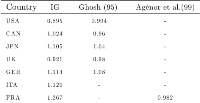
Table 12 – Comparison of with the literature . . . 31
Table 13 – Wald test (p-value) - Per capita time series, in 2000 U.S. dollars. . . .32
Table 14 – Wald test (p-value) - Time series in U.S. dollars (not per capita) . . . 32
Chapter 2 Table 1 – Choice of the autoregressive order . . . 55
Table 2 – Results for the global stationarity test. . . .56
Table 3 – Results for the unconditional mean test . . . 57
Table 4 – Koenker-Xiao test . . . 58
Table 5 – Quarters during which the discounted public debt-GDP ratio is larger than the 0.4-th conditional quantile forecast (yt>Dte ) . . . 59
Table 6 – Out-of-sample forecast of Brazilian debt (% GDP) . . . 62
Table 7 – Summary of the Monte Carlo results . . . 73
Chapter 3 Table 1 – Size investigation . . . 91
Table 2 – Results of the VQR test. . . .96
Table 3 – Backtests comparison . . . 96
Table 4 – Loss Function L(Vt) . . . 98
List of Figures
Chapter 1
Figure 1 –CAt forUK . . . 20
Figure 2 – Global shocks (sample 2) and U.S. recessions . . . 23
Chapter 2 Figure 1 – Example of a QAR(1) model . . . 47
Figure 2 – Separating periods of nonstationarity. . . .47
Figure 3 – Out-of-sample forecast ofyt. . . 50
Figure 4 – Brazilian federal debt (% GDP) . . . 54
Figure 5 – Debt ceiling (Dte ) and discounted debt-GDP ratio (yt) . . . 58
Figure 6 – Out-of-sample forecast of Brazilian debt . . . 60
Figure 7 – Histograms with the frequency ofRi. . . 73
Chapter 3 Figure 1 – Periods of risk exposure . . . 85
Figure 2 – Size-corrected Power Curves - Method 1 . . . 93
Figure 3 – S&P500 daily returns (%) . . . 94
Figure 4 – S&P500 daily returns and VaR (99%) . . . 96
Figure 5 –Wt(RiskMetrics-VaR 99%) . . . 97
Figure 6 –Rtand Vt(RiskMetrics-VaR 99%) . . . 97
Figure 7 – Size-corrected Power Curves - Method 2 . . . 105
Introduction
This thesis is composed of three essays referent to the subjects of macroeconometrics and …nance. In each essay, which corresponds to one chapter, the objective is to investigate and analyze advanced econometric techniques, applied to relevant macroeconomic questions, such as the capital mobility hypothesis and the sustainability of public debt. A …nance topic regarding portfolio risk management is also investigated, through an econometric technique used to evaluate Value-at-Risk models.
The …rst chapter investigates an intertemporal optimization model to analyze the current account. Based on Campbell & Shiller’s (1987) approach, a Wald test is conducted to analyze a set of restrictions imposed to a VAR used to forecast the current account. The estimation is based on three di¤erent procedures: OLS, SUR and the two-way error decomposition of Fuller & Battese (1974), due to the presence of global shocks. A note on Granger causality is also provided, which is shown to be a necessary condition to perform the Wald test with serious implications to the validation of the model. An empirical exercise for the G-7 countries is presented, and the results substantially change with the di¤erent estimation techniques. A small Monte Carlo simulation is also presented to investigate the size and power of the Wald test based on the considered estimators.
The second chapter presents a study about …scal sustainability based on a quantile autoregression (QAR) model. A novel methodology to separate periods of nonstationarity from stationary ones is proposed, which allows one to identify trajectories of public debt that are not compatible with …scal sustainability. Moreover, such trajectories are used to construct a debt ceiling, that is, the largest value of public debt that does not jeopardize long-run …scal sustainability. An out-of-sample forecast of such a ceiling is also constructed, and can be used by policy makers interested in keeping the public debt on a sustainable path. An empirical exercise by using Brazilian data is conducted to show the applicability of the methodology.
Chapter 1
An econometric contribution to the
intertemporal approach of the current account
1Abstract
This paper investigates an intertemporal optimization model to analyze the current account through Campbell & Shiller’s (1987) approach. In this setup, a Wald test is conducted to analyze a set of restrictions imposed to a VAR, used to forecast the current account for a set of countries. We focused here on three estimation procedures: OLS, SUR and the two-way error decomposition of Fuller & Battese (1974). We also propose an original note on Granger causality, which is a necessary condition to perform the Wald test. Theoretical results show that, in the presence of global shocks, OLS and SUR estimators might lead to a biased covariance matrix, with serious implications to the validation of the model. A small Monte Carlo simulation con…rms these …ndings and indicates the Fuller & Battese procedure in the presence of global shocks. An empirical exercise for the G-7 countries is also provided, and the results of the Wald test substantially change with di¤erent estimation techniques. In addition, global shocks can account up to 40% of the total residuals of the G-7. The model is not rejected for Canada, in sharp contrast to the literature, since the previous results might be seriously biased, due to the existence of global shocks.
JEL Classi…cation: C31, E21, F32, F47.
Keywords: current account, capital mobility, error decomposition, common shocks.
1This article was jointly m ade with João Victor Issler. We would like to thank John C. Driscoll, Luiz Renato Lim a, Fabiana
Fontes Rocha, M aria Cristina Terra, and Carlos C. Gutierrez for insightful advices and helpful com m ents. We are also grateful to the
1
Introduction
The current account can be used by domestic residents to smooth consumption by borrowing from or lending to the rest of the world. Several authors have analyzed the open economy model, initially proposed by Sachs (1982) and later detailed by Obstfeld & Rogo¤ (1994), with a theoretical framework that de…nes the optimal current account from the agents’ intertemporal optimization problem, supposing that agents can freely smooth consumption in the presence of shocks. The comparison of this optimal value with the observed current account allows us to test for consumption optimality.
This approach is encompassed by several classes of small open economy models,2 and the most basic
version is the present value model (PVM) of the current account. Although the literature of PVMs is relatively extensive, the following papers should be mentioned (suggesting an overall rejection of the model for developed countries): She¤rin & Woo (1990) perform a study of the current account of Belgium, Canada, Denmark and UK. The results indicate a rejection of the model for Denmark, Canada and UK, whereas the PVM could not be rejected for Belgium. Otto (1992) tests the PVM for the USA and Canada, and rejects the model in both countries. Ghosh (1995) investigates the current account of 5 major industrialized countries: USA, Canada, Japan, Germany and UK, and the results suggest rejection of the model in all countries, except for the USA.
On the other hand, some papers document results supporting the PVM, in contrast to the previous …ndings, such as Ghosh & Ostry (1995) that test it for 45 developing countries and do not reject it for about 2/3 of the countries. Hussein & Mello (1999) also test the PVM for some developing countries (Chile, Greece, Ireland, Israel, Malaysia, Mexico, South Africa, South Korea and Venezuela), and …nd evidences to support the PVM. In the same line, Agénor et al. (1999) focus on the current account of France, concluding that the PVM holds and the analyzed country was perfectly able to smooth consumption.3
Notwithstanding the lack of consensus on the macroeconomic front, what happens on the "econometric side"? Is it possible that an inappropriate econometric technique leads to wrong conclusions regarding the rejection of the PVM? Unlike the mentioned literature, the objective of this paper is to provide an econometric approach to the current account debate. The methodology generally adopted in the literature to analyze the PVM was initially proposed by Campbell & Shiller (1987), and consists of estimating an unrestricted VAR,
2For recent developm ents regarding sm all op en economy m odels see Grohé & Urib e (2003). In addition, see Chinn & Prasad (2003),
which provide an em pirical characterization of the determ inants of current account for a large sam ple of industrial and developing
countries. See also Aguiar & Gopinath (2006), which develop a quantitative m o del of debt and default in a sm all op en economy.
Finally, see Obstfeld & Rogo¤ (1996) and Bergin (2003) for a good discussion ab out new op en economy literature and its em pirical
dim ension.
3In order to deep en the debate, several authors also prop osed extensions to the standard PVM m odel. A short list includes Ghosh &
Ostry (1997), which consider precautionary saving, Grub er (2000) includes habit form ation, Bergin & She¤rin (2000) allow for a tim
e-varying world interest rate and consider tradable and non-tradable goods, ·I¸scan (2002) m odi…es the basic m odel introducing durables
and also nontraded goods. M ore recently, Nason & Rogers (2006) prop ose a real business cycle (RBC) m odel, which nests the basic
PVM , including non-separable preferences, shocks to …scal p olicy and world interest rate, and im p erfect capital m obility, explanations
broadly presented in the literature for the rejection of the PVM . According to Nason & Rogers (2006), although each susp ect m atters
whose parameters are used in the construction of the optimal current account, and perform a Wald test to investigate a set of restrictions imposed to the VAR, testing whether the optimal current account equals the observed series.
However, the presence of common shocks in the econometric model can play a crucial role, and is widely recommended in the literature to explain business cycles ‡uctuations. For instance, Centoni et al. (2003) investigate whether co-movements observed in the international business cycles are the consequences of common shocks or common transmission mechanisms. Similarly to most studies (such as King et al. 1991), Centoni et al. (2003) con…rm that permanent shocks are the main source of the business cycles, accounting for a 50% e¤ect in a panel of European countries. The authors also show that the domestic component is responsible for most of the business cycle e¤ects of transitory shocks for all the G-7 countries, whereas the foreign component dominates the cyclical variability that is due to permanent shocks in France, Germany and Italy.4
This way, seems to exist a consensus in the literature regarding a common world component that might partially explain current account ‡uctuations. This common (or global) shock is ignored in the OLS estima-tion (widely used in the literature), but could be considered in a SUR approach. In fact, along this paper we stress the fact that in the estimation process an econometrician might consider a set of countries separately (OLS) as well as jointly (e.g., SUR), in order to capture contemporaneous correlations of the residuals of the VAR. However, due to the possible …nite sample bias of the OLS and SUR covariance matrices (see Driscoll & Kraay, 1998), we also investigate the two-way error decomposition of Fuller & Battese (1974), hereafter FB, which can properly treat the existence of common shocks in the estimation process.
Therefore, we aim to contribute to the current account debate by investigating the estimation of a PVM through three di¤erent techniques (OLS, SUR and FB). In addition, we propose a quite original note on Granger causality, which is showed to be a necessary condition to perform the Wald test of Campbell & Shiller (1987). In addition, we present some theoretical results to show that (in the presence of common shocks) OLS and SUR estimators might produce a biased covariance matrix, with serious implications to the validation of the model.
A small Monte Carlo simulation con…rms these …ndings and indicates the FB procedure in the presence of global shocks. We also provide an empirical exercise for the G-7 countries, and (indeed) the results substantially change with di¤erent estimation techniques. In addition, global shocks can account up to 40% of the total residuals of the G-7, con…rming the importance of such shocks in the estimation process. The model is not rejected for Canada, in sharp contrast to the literature, since the previous results might be seriously biased, due to the existence of global shocks.
4In the sam e sense, Canova & Dellas (1993) docum ent that after 1973 the presence of com m on disturbances, such as the …rst oil shock,
plays a role in accounting for international output co-m ovem ents. Glick & Rogo¤ (1995) study the current account resp onse to di¤erent
productivity shocks in the G-7 countries, based on a structural m odel including global and country-sp eci…c shocks. Furtherm ore, Canova
& M arrinan (1998), which investigate the generation and transm ission of international cycles in a multicountry m odel with production
and consum ption interdep endencies, argue that a com m on com p onent to the shocks and of production interdep endencies app ear to b e
This paper is structured in the following way: Section 2 provides an overview of the macroeconomic model of the current account and discusses some econometric techniques that might be used in the estimation process. Section 3 presents the results of an empirical exercise for the G-7 countries, and Section 4 presents our main conclusions.
2
Methodology
2.1
Present Value Model
The Present Value Model (PVM) adopted to analyze the intertemporal optimization problem of a repres-entative agent is based on Sachs (1982), considering the perfect capital mobility hypothesis across countries. In this context, countries save through ‡ows of capital in their current accounts, according to their expect-ations of future changes in net output. Thus, the current account is used as an instrument of consumption smoothing against possible shocks to the economy, and can be expressed by
CAt=Bt+1 Bt=Yt+rBt It Gt Ct (1)
whereBtrepresents foreign assets,Yt gross domestic product (GDP),rthe world interest rate, It total investment,Gtthe government’s expenses andCtaggregated consumption.
The consumption path, related to the dynamics of the current account, can be divided into two com-ponents: the trend term, generated by the di¤erence between the world interest rate and the rate of time preference, and the smoothing component, related to the expectations of changes in permanent income. This paper only studies the second component e¤ect, by isolating from the current account, the trend component in consumption. Thus, the optimal current account (only associated with the consumption smoothing term) is given by
CAt =Yt+rBt It Gt Ct (2)
where is a parameter that removes the trend component in consumption.5 The net output Zt, also known in the literature as national cash ‡ow, is de…ned by
Zt Yt It Gt (3)
Substituting the optimal consumption expression in equation (2), it can be shown that the present value relationship between the current account and the future changes in net output is given by (see Ghosh & Ostry (1995) for further details):
CAt = 1 X
j=1
( 1 1 +r)
jE
t( Zt+jjRt) (4)
whereRtis the agent’s information set. It should be mentioned that the main assumptions of the model are time-separable preferences, zero depreciation of capital, and complete asset markets. A quadratic form is also adopted for the utility function, without precautionary saving e¤ects (see Ghosh & Ostry, 1997).
According to equation (4), the optimal current account is equal to minus the present value of the expected changes in net output. For instance, the representative agent will increase its current account, accumulating foreign assets, if a future decrease in income is expected, and vice-versa.
2.2
Econometric Model
The econometric model is based on the methodology developed by Campbell & Shiller (1987), which suggest an alternative way to verify a PVM when the involved variables are stationary. The idea is to test a set of restrictions imposed to a Vector Auto Regression (VAR), used to forecast the current account through equation (4). The advantage of this approach is that, although the econometrician does not observe the agent’s information set, this framework allows us to summarize all the relevant information through the variables used in the construction of the VAR.
However, to apply this methodology, the VAR must be stationary. Hence, the …rst empirical implication is to verify whether Zt is a weakly stationary variable. The current account (in level) must also be a stationary variable, since it can be written as a lineal combination of stationary variables (via equation (4)). The stationarity of these variables can be checked later by unit root tests. Campbell & Shiller (1987) argue that series represented by a Vector Error Correction Model (VECM) can be rewritten as an unrestricted VAR. Thus, consider the following VAR representation:6
" Zi t CAi t # = "
ai(L) bi(L)
ci(L) di(L) # " Zi t 1 CAi t 1 # + " i 1 i 2 # + " "i 1t "i 2t # (5)
where the index i represents the analyzed country and ai(L), bi(L), ci(L) and di(L) are polynomials of order p. Hence, the estimation of the VAR must be preceded by the estimation of , which occurs in the cointegration analysis between Ct and(Yt+rBt It Gt). The model VAR(p) can be described as a VAR(1), in the following way:
2 6 6 6 6 6 6 6 6 6 6 6 6 6 6 6 6 6 4 Zi t .. . .. . Zi t p+1
CAi t .. . .. . CAi t p+1
3 7 7 7 7 7 7 7 7 7 7 7 7 7 7 7 7 7 5 = 2 6 6 6 6 6 6 6 6 6 6 6 6 6 6 6 4 ai
1 aip bi1 bip
1
. .. 0
1 ci
1 cip di1 dip
1
0 . ..
1 3 7 7 7 7 7 7 7 7 7 7 7 7 7 7 7 5 2 6 6 6 6 6 6 6 6 6 6 6 6 6 6 6 6 6 4 Zi t 1 .. . .. . Zi t p CAi t 1 .. . .. . CAi t p 3 7 7 7 7 7 7 7 7 7 7 7 7 7 7 7 7 7 5 + 2 6 6 6 6 6 6 6 6 6 6 6 6 6 6 6 4 i 1 0 .. . 0 i 2 0 .. . 0 3 7 7 7 7 7 7 7 7 7 7 7 7 7 7 7 5 + 2 6 6 6 6 6 6 6 6 6 6 6 6 6 6 6 4 "i 1t 0 .. . 0 "i 2t 0 .. . 0 3 7 7 7 7 7 7 7 7 7 7 7 7 7 7 7 5 (6)
or, in a compact form:
Xt=AXt 1+ +"t (7)
6It should b e m entioned that, hereafter, CA
twill b e constructed considering the param eter , to rem ove the trend com p onent in
whereXt h
Zi
t Zt pi +1 CAit CAit p+1
i0
,Ais the companion matrix, represents a vector of intercepts, and"tis a vector that contains the residuals. The VAR(1) is stationary by assumption, and the equation (7) can be rewritten removing the vector of means :
(Xt ) =A(Xt 1 ) +"t (8)
where = (I A) . The forecast of the modelj periods ahead is given by
E[(Xt+j jHt) =Aj(Xt ) (9)
whereHt is the econometrician’s information set (composed of current and past values ofCAand Z), contained in the agent’s information set Rt. De…neh0 as a vector with 2pnull elements, except the …rst:
h0=h 1 0 : : : 0 i. Then, one can select Ztin the vectorXt, in the following way:
Zt=h0Xt) Zt+j=h0Xt+j)( Zt+j Z) =h0(Xt+j ) (10) where the vector contains the means Z and CA . Thus, applying the conditional expectation in the previous expression, it follows that:
E[( Zt+j Z)jHt] =E[h0(Xt+j )jHt] =h0E[(Xt+j )jHt] =h0Aj(Xt ) (11) where the last equality comes from equation (9). In order to calculate the optimal current accountCAt, one can take expectations of equation (4):
E(CAt jHt) =CAt = 1 X
j=1
( 1 1 +r)
jE( Z
t+jjHt) (12)
The …rst equality comes from the fact thatCAt is contained inHt, and the second is given by the law of iterated expectations (Ht Rt). Applying the unconditional expectation in the previous expression:
E(CAt) = 1 X
j=1
( 1 1 +r)
jE( Z
t+j)) CA = 1 X
j=1
( 1 1 +r)
j
Z (13)
Combining equation (12) with equation (13), it follows that:
(CAt CA ) = 1 X
j=1
( 1 1 +r)
jE( Z
t+j Z jHt) (14)
Applying the expression (11) in the equation above:
(CAt CA ) = 1 X
j=1
( 1 1 +r)
jh0Aj(X
t ) = h0(
A 1 +r)(I
A 1 +r)
1(X
t ) (15)
where the last equality is due to the convergence of an in…nite sum, since the variables ZtandCAtare stationary. Rewriting the previous equation in a simpli…ed form:
K= h0( A 1 +r)(I
A 1 +r)
1 (17)
where the vector K is derived from the world interest rate r and the matrixA. To formally test the model, one can analyze the null hypothesis (CAt CA ) = (CAt CA). De…ne g0 as a vector with2p null elements, except the (p+ 1)thelement, that assumes a unit value. Thus, under the null hypothesis, it follows that:
(CAt CA ) = (CAt CA) =g0(Xt ) (18)
Combining equations (16) and (18), the model can be formally tested through a set of restrictions imposed to the coe¢cients of the VAR:
g0(Xt ) = h0( A
1 +r)(I A 1 +r)
1(X
t ))g0(I A
1 +r) = h
0( A
1 +r) (19)
Applying the structure of matrixAinto equation (19), the following restrictions7 can be derived:
ai =ci ;i= 1:::p
bi=di ;i= 2:::p
b1=d1 (1 +r)
(20)
Another important implication of the model is that the current account Granger-cause changes in net output, or in other words,CAthelps to forecast Zt. This causality can be tested by means of the statistical signi…cance of the b(L) coe¢cients. Therefore, the implications of the intertemporal optimization model, according to Otto (1992), can be summarized by:8
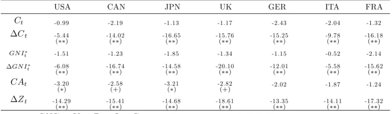
1. Verifying the stationarity ofCAt and Zt, through unit root tests; 2. Checking ifCAt Granger-cause Zt;
3. Analyzing the cointegration betweenCtand(Yt+rBt It Gt), and calculating the parameter ; 4. Formally investigating, by means of a Wald test, the equality of the optimal and observed current accounts, given by restrictions (20).
2.3
A note on Granger Causality and Wald Tests
The optimal current account is generated from the vectorK(see expressions (16) and (17)), which depends on matrix A and the world interest rate r. However, it should be noted that an estimated coe¢cient for matrix A could not be statistically signi…cant. These results could seriously compromise the subsequent optimal current account analysis, as it follows.
The Granger causality between the current account and net output(CAtGranger-cause Zt)is a prim-ordial implication of the theoretical model, and as argued before, can be alternatively tested through the signi…cance of the b(L) coe¢cients.9 Moreover, if this implication is not empirically observed, the model
7These restrictions can b e veri…ed by a Wald test.
8It is in fact a set of testable im plications of the PVM . Therefore, the statistical acceptance of the m odel occurs only if all of these
im plications could b e veri…ed.
should be rejected irrespective of any other results, since equation (4) is the theoretical foundation of the whole study. In this case, the current account could not help to predict variations in net output, suggesting that the agents are badly described by the model. Thus, one should not construct the optimal current account and perform a comparison with the observed series. Unfortunately, this is done in several papers presented in the literature.
To study this topic more carefully, a simple VAR(1) is initially presented. The Granger causality between
CAt and Zt, in this case, will be determined by the statistical signi…cance of theb1 coe¢cient.
" Zt
CAt #
=
" a1 b1
c1 d1
# " Zt 1
CAt 1
#
+
"
1
2
#
+
" "1t
"2t #
: (21)
In this case, the VAR is represented in a compact form byXt=AXt 1+ +"tand, after some algebraic manipulations, the vectorK takes the form:
K= h0( A 1 +r)(I2
A 1 +r)
1=h i; (22)
where
= a1(1 +r d1) b1c1
(1 + 2r d1+r2 rd1 a1 a1r+a1d1 b1c1)
; (23)
= a1b1 b1(1 +r a1)
(1 + 2r d1+r2 rd1 a1 a1r+a1d1 b1c1): (24)
If the Granger causality is rejected by the data (e.g.,b1 is not signi…cant), then equation (25) indicates
that = 0, or in other words,CAt is not a function ofCAt. In this case, the optimal current account would be given by
(CAt CA ) =K(Xt ) = h
0 i
"
Zt Z
CAt CA
#
= ( Zt Z): (25)
Hence, if = 0the null hypothesis (CAt CA) = (CAt CA)is always rejected, since under Ho should be equal to one (and should be zero). A further analysis of the vectorKfor a VAR(2) is presented in appendix, in a similar way. The generalization of this cautionary note for a VAR(p) is straightforward, and can be summarized by Proposition 1. According to Hamilton (1994), in the context of a bivariate VAR(p), if one of the two variables does not Granger-cause the other, then the companion matrix is lower triangular (e.g., b(L) = 0). Thus, the i coe¢cients of the vector K (i = 1; : : : ; p) are always zero, because of the algebraic structure of the vector, as also detailed in appendix.
Proposition 1 Consider the VAR representation (5) of the intertemporal model of current account. The Granger causality from the current account(CAt)to the …rst di¤erence of the net output( Zt)is a necessary
Proof. See Appendix.
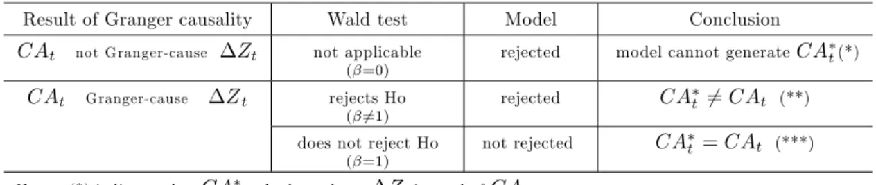
Therefore, if the Granger causality could not be con…rmed by the data set, neither a Wald test should be performed nor the optimal current account should be generated, since the basic assumption of the model is not veri…ed,10 as summarized in table 1.
Table 1 - A note on Granger causality and Wald tests
Result of Granger causality Wald test Model Conclusion
CAt not Granger-cause Zt not applicable
( =0)
rejected model cannot generateCAt(*)
CAt Granger-cause Zt rejects Ho
( 6=1)
rejected CAt 6=CAt (**)
does not reject Ho ( =1)
not rejected CAt =CAt (***)
Notes: (*) indicates thatCAt only dep ends on Z, instead ofCAt
(**) suggests that agents do not sm ooth consum ption;
(***) m eans that agents p erfectly sm ooth consum ption.
2.4
Estimation Method
2.4.1 SUR estimation
The VAR model (5) is usually estimated in the literature, equation-by-equation, using OLS. However, the Seemingly Unrelated Regressions (SUR) technique, originally developed by Zellner (1962), can also be ad-opted, since it is based on a Generalized Least Squares (GLS) estimation applied to a system of equations as a whole, in which the data for several countries is examined simultaneously. The joint estimation is given by stacking the system of equations that compose the VAR (for each country i= 1; : : : ; N) in the following
way: " Zi t CAi t # = "
ai(L) bi(L)
ci(L) di(L) # " Zi t 1 CAi t 1 # + " "i 1t "i 2t # (26)
Then, de…neYi t = Zi t CAi t ! (2 1)
, Xi t= 0 B B B B B B B B B B @ Zi t 1 .. . Zi t pi
CAi t 1
.. .
CAi t pi
1 C C C C C C C C C C A
(2pi 1)
, "i t= "i 1t "i 2t ! (2 1)
and 0i= ai1 : : : aipi b
i
1 : : : bipi c
i
1 : : : cipi d
i
1 : : : dipi (1 4p
i)
1 0Recall Ghosh & Ostry (1995) results, in which the authors test the PVM for 45 developing countries and do not reject it for 29
countries. However, a careful analysis of the tests reveals that only 25 countries (from the entire set of countries) in fact supp ort the
Granger causality im plication (at 5% level). This way, the pap er should conclude that (at m ost) in only 18 countries (instead of 29)
This way, the VAR for a countryican be represented by
Yi
t (2 x 1)=
X10
t 0
0 X10 t
!
(2 x 4pi)
i
(4pix 1)+ "
i t
(2 x 1) (27)
Furthermore, the system of equations for a given set ofN countries can be expressed by 0 B B @ Y1 t .. . YN t 1 C C A
(2N x 1)
= 0 B B B B B B B @
X10
t 0 : : : 0
0 X10 t ..
. . .. 0 ...
0 XN0
t 0
0 : : : 0 XN0
t 1 C C C C C C C A
(2N x 4P)
0 B B @ 1 .. . N 1 C C A
(4P x 1)
+ 0 B B @ "1 t .. . "N t 1 C C A
(2N x 1)
(28)
or in a compact form Y = X +". The name SUR comes from the fact that each equation in the previous system has its own vector of coe¢cients, which might suggest that the equations are unrelated. Nevertheless, correlation across the errors in di¤erent equations can provide links that can be exploited in estimation. It should be noted that
N P i=1
pi =P, wherepi is the number of lags of the VAR, for a countryi. The residuals"have mean zero and are serially uncorrelated, with covariance matrix given byE(""0) = 2 .
Hence, the GLS estimator of and its variance-covariance matrix are given by
e= X0 1X 1X0 1Y (29)
E(e )(e )0= 2 X0 1X 1 (30)
In general, the(N N)matrix is unknown and the last expression cannot be directly applied. However, e can be calculated by an estimate of theijth element of , given by
b wij= e
0 iej
T ; wherei; j= 1; : : : ; N (31)
whereei is a(T 1) vector containing the residuals of theith equation estimated by OLS. In this case, a feasible SUR estimator of is obtained as
e = X0b 1X 1X0b 1Y (32)
E(e )(e )0 = 2 X0b 1X 1 (33)
The OLS estimator, on the other hand, is given by
b= (X0X) 1X0Y (34)
E(b )(b )0= 2(X0X) 1X0 X(X0X) 1 (35)
The di¤erence between their variance-covariance matrices is a positive semide…nite matrix, and can be expressed by
E(b )(b )0 E(e )(e )0= 2 0 (36)
where = (X0X) 1
X0 X0 1X 1X0 1, indicating the gain in e¢ciency of SUR estimators in
2.4.2 Caveats of SUR estimation
The SUR estimator generally exhibits a good performance whenN is small relative toT, but in fact becomes not feasible whenT <(N+ 1)=2. Even when the SUR model is correctly speci…ed, its performance might be poor due to a very large number of free parameters to be estimated, in comparison to the time dimension. In other words, asN becomes large for a …xed value ofT, the estimated covariance matrix becomes “nearly” singular, introducing a bias into the standard error estimates. This way, the …nite sample performance of the OLS and SUR estimators deteriorates rapidly as the size of the cross-sectional dimension increases.
Driscoll & Kraay (1998) investigate …nite-sample properties of variance estimators, concluding that both OLS and SUR estimators indeed exhibit substantial downward …nite sample bias, even for moderate values of cross-sectional dependence, and are outperformed by a spatial correlation consistent estimator proposed in their article, based on the nonparametric technique of Newey & West (1987) and Andrews (1991).
The main idea is to obtain consistent estimates of theN N matrix of cross-sectional correlations by averaging over the time dimension. This way, the estimated cross-sectional covariance matrix can be used to construct standard errors, which are robust to the presence of spatial correlation. Driscoll & Kraay (1998)’s approach, in contrast to SUR, might be applicable in situations such as cross-country panel data models with a relatively large number of countries.
In this paper, however, we focus on a panel model with smallN and largeT, but in order to deal with possible …nite sample bias of the covariance matrix, we also investigate a two-way error decomposition (next described) that can properly deal with cross-country correlations.
2.4.3 Fuller & Battese (1974) and the two-way error decomposition
The performance of any estimation procedure depends on the statistical characteristics of the error compon-ents in the model. In this section, we adopt the Fuller & Battese (1974) method to consider individual and time-speci…c random e¤ects into the error disturbances, in which parameters can e¢ciently be estimated by using a feasible GLS framework.
In dynamic panel models, the presence of lagged dependent variables might lead to a non-zero correlation between regressors and error term. This could render OLS estimator for a dynamic error-component model to be biased and inconsistent (see Baltagi, 2001, p. 130), due to the correlation between the lagged dependent variable and the individual speci…c e¤ect. In addition, a feasible GLS estimator for the random-e¤ects model under the assumption of independence between the e¤ects and explanatory variables would also be biased. In these cases (with largeN and shortT), Andersen & Hsiao (1981) suggests …rst di¤erencing the model to get rid of the individual e¤ect. On a di¤erent approach, but still in a framework of dynamic models with largeN and shortT, Holtz-Eakin et alli (1988) investigate panel VAR (PVAR) models, in order to provide more ‡exibility to the VAR modeling for panel data. See also Hsiao (2003, p. 70,107) for further details.
& Battese (1974) approach to our system of equations (28). These authors establish su¢cient conditions for a feasible GLS estimator to be unbiased and exhibit the same asymptotic properties of the GLS estimator in a crossed-error model, i.e., in which an error decomposition is considered to allow for individual e¤ects that are constant over cross sections or time periods. To do so, initially consider the stacked modelY =X +";from the system of equations (28), where Y = (y1;1;y1;2;:::;y1;T;:::;y2N;T);X = (x1;1;x1;2;:::;x1;T;:::;x2N;T); and xi;t are p 1 vectors. The Fuller & Battese (1974) two-way random error decomposition is given by
"i;t =vi+et+ i;t, in which E(""0 jX) .
Thus, the model is a variance components model, with the variance components 2; 2
v; 2eto be estimated. A crucial implication of such a speci…cation is that the e¤ects are not correlated with the regressors. For random e¤ects models, the estimation method is a feasible generalized least squares (FGLS) procedure that involves estimating the variance components in the …rst stage and using the estimated variance covariance matrix thus obtained to apply generalized least squares (GLS) to the data. It is also assumed thatE(vi) =
0;E(v2
i) = 2v; E(vivj) = 0;8i 6= j;vi is uncorrelated with i;t;8i; t; and also E(et) = 0;E(e2t) = 2e;
E(etes) = 0;8t6=s;etis uncorrelated withvi and i;t;8i; t:11
Contrary to Wallace & Hussain (1969) or Swamy & Arora (1972), Fuller & Battese (1974) also consider the case in which 2
vand/or 2eare equal to zero.12 The estimators for the variance components are obtained by the …tting-of-constants method, with the provision that any negative variance components is set to zero for parameter estimation purposes. First, the least square residuals are de…ned by: b" = M12(I
X[X0M
12X] 1X0M12]Y;bv= (M12+M1:)(I X[X0(M12+M1:)X] 1X0(M12+M1:)]Y;be= (M12+M:2)(I
X[X0(M
12+M:2)X] 1X0(M12+M:2)]Y. Next, Fuller & Battese compute the unbiased estimators for the
variance components: b2 = (N 1)(b"Tb"0 1)
1; b
2
v = b
vbv0 [T(N 1)
2]b2 T(N 1) T 1 ; b
2
e = b
eeb0 [N(T 1)
3]b2
N(T 1) N 2 where 1 rank(X0M
12X); 2 rank(X0M:2X); 3 rank(X0M1:X); 1 trf[X0(M12+M1:)X] 1X0M1:Xg; 2
trf[X0(M12+M:2)X] 1X0M:2Xg.
Once the component variances have been estimated, we form an estimator of the composite residual covariance, and then GLS transform the dependent and regressor data. The respective GLS estimator is given by bF B= (X0 1X) 1X0 1Y and, thus, the FB estimator is the related feasible GLS estimatorbbF B, in which is estimated throughb2;b2v;andb
2
e. Fuller & Battese (1974) show that their estimator is consistent,
1 1The authors also de…ne the following mutually orthogonal, sym m etric and idem p otent m atricesM
::= J22N TN T ;M1:= I2NTJT
M::;M:2= J2N2NIT M::;M12=I2N T I2NTJT J2N2NIT +M::; whereI2NandITare identity m atrices of order2N Tand
T, resp ectively; andJ2N andJTare(2N 2N)and(T T)m atrices having all elem ents equal to one. The covariance m atrix =
2I
2N T+ 2v(I2N JT)+ 2e(J2N IT)can b e expressed by 2M12+( 2+T 2v)M1:+( 2+2N 2e)M:2+( 2+T 2v+2N 2e)M::,
or even, = 1M12+ 2M1:+ 3M:2+ 4M::, where 1 2; 2 ( 2+T 2v); 3 ( 2+ 2N 2e); 4 ( 2+T 2v+ 2N 2e).
1 2Baltagi (1981) p erform ed a M onte Carlo study on a single regression equation with two-way error com p onent disturbances and
studied the prop erties of several estim ators, including OLS and six feasible GLS estim ators: Fuller & Battese (1974), Swamy-Arora
(1972), Wallace & Hussain (1969), am ong others. The results suggest that OLS standard errors are biased and all FGLS are asym
ptot-ically e¢ cient and p erform ed relatively well in …nite sam ples, m aking it di¢ cult to choose am ong them . The m ethods di¤er only in the
sp eci…cations estim ated in evaluating the residuals: The Swamy-Arora estim ator of the com p onent variances uses residuals from the
within (…xed e¤ect) and b etween (m eans) regressions, while the Wallace-Hussain estim ator uses only OLS residuals. In general, they
unbiased and asymptotically equivalent to the GLS estimator. In addition, the estimated covariance matrix of coe¢cients is unbiased, since it is based on unbiased and consistent estimators b2;b2v;b
2
e. Table 2 - Comparison of OLS, SUR and FB covariance matrix of residuals
E("i;t"j;sjX) OLS SUR FB
i=j;t=s 2i i2 ( 2v+ 2e+ 2)
i6=j;t=s 0 2
i;j 2e
i=j;t6=s 0 0 2
v
i6=j;t6=s 0 0 0
In the SUR approach, the covariance structure allows for conditional correlation between the contem-poraneous residuals for cross-section, but restricts residuals in di¤erent periods to be uncorrelated. On the other hand, following the argument of Wooldridge (2002, p. 259), rather than depending on N(N + 1)=2
variances and covariances, as would be the case in a SUR analysis, of the Fuller & Battese (1974) approach only depends on three parameters, 2; 2
v; 2e, regardless of the size of N. This parsimonious feature might be useful for a large panel model, withN; T ! 1. See Baltagi (1980), which investigates a SUR model with error components, and also Pesaran and Smith (1995) and Phillips and Moon (1999) for panel data with largeT andN. 13 We next show some important results of the OLS and SUR estimators for the system of equations (28), under the Fuller & Battese error decomposition.
De…nition 3: De…ne the bias on the estimated covariance matrix by: B V ar( ) E(V ard( )jX);
De…nition 4: De…ne 2N 2
e=( 2+T 2v+ 2N 2e);
Assumption A1: (X0X)and(X0JX)are positive de…nite matrices, whereJ J
2N IT;
Assumption A2: (i) tr[(X0X) 1X0JX I] >0; and (ii) T > 2p, where p is the number of lags of the VAR14;
Proposition 2 (OLS) Assume the Fuller & Battese (1974) two-way random error decomposition. (i) If ( 2; 2
e; 2v) >0 , then, bOLS is inconsistent; (ii) if 2v = 0 and ( 2; 2e)>0, then, V ard( OLS) is biased;
(iii) if 2
v= 0;( 2; 2e)>0; and A1-A2 hold, then,diag(@B@OLS2
e )>0, i.e., an increase of the common shock 2
e (and, thus, ) induces an upward bias on all estimated (OLS) variances; and (iv) if ( 2v; 2e) = 0 and
2>0 , then, V ard(
OLS)is unbiased. Proof. See Appendix.
As already expected, substituting OLS residuals instead of the true disturbances introduces bias in the corresponding estimates of the variance components and, thus, on the covariance matrix of coe¢cients. See
1 3For panels with largeN andT, several approaches m ight b e considered: (i) sequential lim its, in which a sequential lim it theory is
considered; diagonal-path lim its, which allows the two indexes to pass to in…nity along a sp eci…c diagonal path in the two dim ensional
array; or joint lim its, in which b oth indexes pass to in…nity simultaneously. See Hsiao (2003, p.295) for further details, and also Phillips
& M oon (1999), which provide su¢ cient conditions that ensures the sequential lim its to b e equivalent to joint lim its.
1 4Recall from (28) that PN
i=1
pi=P, wherepiis the numb er of lags of the VAR for a given country i. By assum ing thatpi=p;8i;
Maddala (1971) and Baltagi (2001, p.35) for further details. On the other hand, if assumptions A1-A2 do not hold, then, we cannot guarantee that all estimated variances are upwarded biased. It could be the case that some variances do exhibit a positive bias, whereas others are not a¤ected at all, or even show a negative bias.15
Assumption A3: 2I
2N+ 2eJ2N b >0;
Assumption A4: 2I2N+ 2eJ2N =b;
Assumption A5: b is a positive semide…nite matrix; and > (tr((X0X) 1X20JXN(2) 2N TN Tk))+2N(2N T k); where
k= 4N p andJ J2N IT;
Proposition 3 (SUR) Assume the Fuller & Battese (1974) two-way random error decomposition. (i) If ( 2; 2
e; 2v)>0 , then, bSU R is inconsistent; (ii) if 2v= 0; ( 2; 2e)>0 and A3 hold, then, V ard( SU R) is
biased. In addition, if A2(ii) and A5 also hold, then, (BOLS BSU R)>0, i.e., the bias of SUR estimated
variances of is not greater than the respective OLS bias; (iii) if 2
v = 0; ( 2; 2e)>0 and A4 hold, then, d
V ar( SU R)is unbiased; and (iv) if( 2v; 2e) = 0 and A4 hold, then,V ard( SU R) =V ard( OLS) is unbiased.
Proof. See Appendix.
Note that as long astr(X(X0X) 1X0J)increases, the exigency for decreases, in order to guarantee that
(BOLS BSU R)>0. In other words, if the common shock is relatively signi…cant in the disturbance term, then, the SUR technique might produce a less biased covariance matrix in respect to the OLS approach. Now, we present su¢cient conditions for the Fuller & Battese (1974) estimator to be unbiased and consistent when applied to our setup. Initially, lets de…ne bF B as the unfeasible Fuller & Battese (1974) estimator, and bbF B as the feasible FB estimator, based on the estimated e¤ects b
2
v;b
2
e and b
2
. Assumption A6: X0 1X is nonsingular, and plim(X0 1
X
T ) =Q , when T ! 1, with …xedN; where
Q is a …nite positive de…nite matrix;
Assumption A7: et and i;t are independent and normally distributed; Assumption A8: plim[(X0bT1X) (X0 T1X)] = 0andplim[(X0pb 1"
T ) ( X0 1
" p
T )] = 0; whereb =b
2
I2N T+ b2v(I2N JT) +b2e(J2N IT)is the estimated Fuller & Battese (1974) covariance matrix.
Proposition 4 Assume the Fuller & Battese (1974) two-way random error decomposition. Thus, it follows that: (i) if 2
v= 0;( 2; 2e)>0;and A6 holds, then, (i) the FB estimatorbF Bis unbiased and consistent; (ii)
if 2
v= 0;( 2; 2e)>0;and A6-A7 hold, then, the FB estimatorbF B is asymptotically normally distributed,
i.e., bF B N( ; (X0 1X) 1); and (iii) if A6, A7 and A8 hold, then, the feasible FB estimator bb
F B is
asymptotically equivalent to bF B.
1 5Note that if X = [1; :::;1]0, then, it follows that(X0X) 1 = 1=2N T and tr[XX0J] =tr[(J
2N T)(J2N IT)] =tr[(J2N
JT)(J2N IT)] =tr[(J2NJ2N) (JTIT)] =tr(J2NJ2N)tr(JTIT) =T tr(J2NJ2N) =T(2N)(2N). Thus,tr[(X0X) 1X0JX I] =
tr[(X0X) 1X0JX] tr(I) =tr[X0JX]=2N T 2N T=tr[XX0J]=2N T 2N T = 2N(2N T)=2N T 2N T= 2N(1 T)<0. In
other words, if A1-A2 do not hold we cannot guarantee thatdiag(@@B2
Proof. See Appendix.
Note that if one assumes that the residuals of each country are serially uncorrelated, then, E("i;t"i;s j
X) = 0 ;8t6=s, which means that 2
v= 0.16 In addition, a …xed e¤ect forvi would be more appropriate in this framework, since we are focused on a speci…c set ofN countries (see Baltagi, 2001 p.12). On the other hand, for the time componentetwe assume a random e¤ect in order to avoid a signi…cant loss of degrees of freedom due to the largeT setup.
In order to verify the …nite sample performance of the competing OLS, SUR and FB estimators, we next conduct a small Monte Carlo simulation.
2.5
Monte Carlo simulation
The econometric methodology described in section 2.2 suggests a Wald test to investigate a set of restrictions imposed to the coe¢cients of a VAR, used to forecast the current account. The Wald test veri…es whether or not the optimal current account is statistically equal to the observed current account. Moreover, the Wald test could be conducted based on OLS, SUR and FB estimations for the coe¢cients of the VAR. Therefore, the goal of our experiment is to investigate the power and the size of the Wald test, comparing di¤erent techniques used for the estimation of the VAR (reproduced below for a generic countryi):
" Zi
t
CAi t
#
=
"
ai(L) bi(L)
ci(L) di(L) # "
Zi t 1
CAi t 1
#
+
" "i
1t
"i
2t #
: (37)
One of the critical issues regarding Monte Carlo experiments is that of Data-Generating Processes (DGPs). In our experiment, we construct 100 DGPs, and for each DGP we generate 1,000 samples of the series h Zt CAt
i0
, by sampling random series of "t’s. Moreover, each sample contains 1,000 ob-servations, but, in order to reduce the impact of initial values we consider only the last T = 100 or 200
observations. Thus, the Monte Carlo simulation performs 100,000 replications of the experiment.17
Two important issues regarding the companion matrix of the generated series must be addressed at this point. The …rst one is related to the null hypothesis to be checked by the Wald test: In our simulation, we impose Ho to be true or false by just controlling the impact of the theoretical restrictions into the companion matrix. The magnitude of the theoretical restrictions is given by the gamma parameter, in which = 1
imposes Ho to be true, whereas 6= 1 leads to a false Ho (see appendix for details). The second issue is related to the stationarity of the VAR: In order to apply the econometric methodology, each sample of the experiment must be constructed to generate a covariance-stationary VAR. This way, we show (see also
1 6In addition, the "individual e¤ect" translates in practice into an individual intercept; which is also exp ected to b e zero in our
setup, since all series are supp osed to b e weakly stationary and previously dem eaned.
1 7A hybrid solution using E-Views, R and M atLab environm ents is adopted, since the prop osed simulation is extrem ely com putational
intensive. We proceed as follows: an E-Views code initially generates the tim e series ZtandCAtfor each DGP. Then, it estim ates
the VAR coe¢ cients based on OLS and SUR techniques and save all the replications and the Wald test results in the hard disk. Next,
an R code com putes the FB estim ator and conducts the resp ective Wald test, also saving the results in a text …le. Finally, a M atLab
code reads all the results from the hard disk, com putes the size of the Wald test based on the three estim ators and also constructs the
appendix for details) how to guarantee the stationarity of the VAR by properly "choosing" the eigenvalues of the companion matrix inside the unit circle, and then calculating the coe¢cients of the companion matrix that generate those eigenvalues.
Results
Concerning the size of the Wald test, we calculate the estimated signi…cance level by simply observing the frequency of rejection of the null hypothesis in the 100,000 replications of the experiment under conditions where the null hypothesis is imposed to be true. Regarding the power of the test, we also compute the rejection frequencies, but under conditions where the null hypothesis is now imposed to be false.
Table 3- Size of the Wald test
Model OLS SUR FB
(a) N=2 ; T=100 0.0171 0.0653 0.0534
(b) N=2 ; T=200 0.0154 0.0559 0.0520
(c) N=5 ; T=200 0.0175 0.0620 0.0503
Note: The nom inal size of the test is =5% , in which
em pirical size = (frequency of p-values b elow the (nom inal size) / (M C*DGP);
where (M C*DGP) = 100,000 = total numb er of replications.
Overall, the results suggest that FB-based test has an adequate size in all cases, whereas the OLS-test exhibits a serious …nite sample bias, as already predicted by Proposition 2. In the same line, the SUR-test also seems to show a (small) non-zero bias due to the presence of global shocks, as previously discussed in Proposition 3.
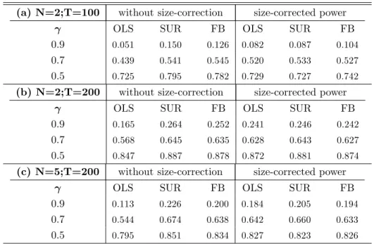
The power investigation can be conducted by controlling the experiment under conditions where the null is imposed to be false, i.e., 6= 1. If the null hypothesis were only ”slightly false” (e.g., = 0:9), one would expect power to be lower than if it were ”grossly false” (e.g., = 0:5). The results of the power investigation corroborate this expectation and are presented in next tables. To adjust for size distortion, we also report a "size-corrected" power.18 The results with size correction are quite similar, suggesting that the Wald test
might exhibit similar power across the considered estimation procedures.
Table 4 - Power of the Wald test
(a) N=2;T=100 without size-correction size-corrected power
OLS SUR FB OLS SUR FB
0.9 0.051 0.150 0.126 0.082 0.087 0.104
0.7 0.439 0.541 0.545 0.520 0.533 0.527
0.5 0.725 0.795 0.782 0.729 0.727 0.742
(b) N=2;T=200 without size-correction size-corrected power
OLS SUR FB OLS SUR FB
0.9 0.165 0.264 0.252 0.241 0.246 0.242
0.7 0.568 0.645 0.635 0.628 0.643 0.627
0.5 0.847 0.887 0.878 0.872 0.881 0.874
(c) N=5;T=200 without size-correction size-corrected power
OLS SUR FB OLS SUR FB
0.9 0.113 0.226 0.200 0.184 0.205 0.194
0.7 0.544 0.674 0.638 0.642 0.660 0.633
0.5 0.795 0.851 0.834 0.827 0.823 0.826
Notes: a) Power = (frequency of p-values b elow the % nom inal size) / (M C*DGP),
b) Gam m a<1 indicates a false Ho.
3
Empirical Results
3.1
Data
All data are from the national accounts of IFS – International Financial Statistics (IMF). The CAt and
Zt series for the G-7 countries are constructed from seasonally adjusted quarterly data (at annual rates), and are expressed in 2000 local currency.19 In addition, all data are converted in per capita real terms, by
dividing it by the implicit GDP de‡ator and the population. It is worth mentioning that the current account data are not directly obtained from the balance of payments data sets, since these series are not available for all of the countries for an extensive period of time, and it would lead to an arbitrary allocation of "net errors and omissions" in the current account.
Sample 1 (G-7): USA, Canada, Japan, United Kingdom, Germany, Italy, and France.
Period: 1980:q1–2007:q1 (set of 7 countries, 109 time periods, with a total amount of2N T = 1;526observations).
Sample 2: USA, Canada, Japan, United Kingdom, and Germany.
Period: 1960:q1–2007:q1 (set of 5 countries, 189 periods, with a total amount of2N T = 1;890observations).
1 9Based on IM F’s World Econom ic Outlook (April, 2005 - statistical app endix), we adopt the following …xed conversion rates (after
31/12/1998) b etween the Euro and the currencies of Germ any, France and Italy: 1 Euro = 1.95583 Deutsche m ark = 6.55957 French
3.2
Granger Causality
One of the four implications of the theoretical model,20 listed by Otto (1992), is thatCA
t helps to forecast
Zt. According to our results, one can verify that the null hypothesis (CAt does not Granger-cause Zt) is rejected at 5% level for Canada and Japan.
Table 5 - Comparison of Results(Ho: CAtdoes not Granger-cause Zt)
Granger Causality (p-value)
Country \ Author IG O G A
USA 0.16944 0.0001 0.0004 -CAN 0.04617 0.21 0.40 -JPN 0.02426 - 0.62 -UK 0.47515 - 0.68 -GER 0.83352 - 0.76 -ITA 0.91321 - - -FRA 0.59218 - - 0.10
Notes: IG m eans Issler & Gaglianone (our results), O refers to Otto (92), G indicates Ghosh (95), A refers to Agénor et al. (1999).
Our results are quite in contrast to the literature, probably due to the di¤erent sample periods. For instance, Otto (1992) rejects Ho for the USA (at 1% level), but does not reject it for Canada. Ghosh (1995) also rejects Ho for the USA (at 1% level) and does not reject it for Canada, Japan, UK and Germany, and Agénor et al. (1999) present a p-value of 0.10 for France. The di¤erent results could possibly be explained by the broader range of our sample period, in comparison to the previous studies, which do not account for all global and idiosyncratic shocks occurred in the last decades: Our sample period covers quarterly data from 1960 until 2007, whereas Otto (1992) considers the period 1950-88, Ghosh(1995) studies the period 1960-88, and Agénor et al. (1999) covers 1970-96.
Thus, our results indicate that, with the exception of Canada and Japan, the current account does not help to forecast the net output of the G-7 countries, indicating that the agents possibly do not have any additional information to predict Zt, other than those contained in the past of their own series. Recall Proposition 1, which states that if the Granger causality implication is not veri…ed, then, the optimal current account should not be generated, since it would lead to spurious results. In the present work, the Granger causality is only veri…ed for Canada and Japan. Thus, for the other countries, the model should be rejected and the optimal current account should not be generated. For instance, the case of UK (sample 1) can be analyzed as an example of spurious result. The VAR(1) estimated for this country is given by
VAR coe¢cients forUK "
Zt
CAt #
=
"
a1= 0:211322 (-2.40) b1= 0:066236 (-1.76)
c1= 0:133631 (-1.12) d1= 0:854978 (16.99)
# " Zt 1
CAt 1
#
+
"
5:477849 (1.67)
2:626709 (0.59)
#
+
" "1t
"2t #
Note: t-statistics in parentheses
wherea1 andd1 are statistically signi…cant, but this is not the case forb1andc1. As described in table
6, the vectorK(recall equation (22)) is extremely sensitive to variations inb1and could generate completely
di¤erent CAt series.21 Assuming b1= 0:066(instead of zero, since b1 is not statistically signi…cant), the
model indicates that = 0:348 (unlike the correct value of = 0).
Table 6- VectorK= [ ; ]for UK
Assumeb1= 0:066 Assumeb1= 0
0:134 0:172
0:348 0:000
Figure 1 -CAt forUK
- 6 0 - 4 0 - 2 0 0 20 40 60
60 65 70 75 80 85 90 95 00 05 UK_CA_OT UK_CA_OT (b1=0)
Note: The picture ab ove exhibits two optim al current accounts
for UK (sam ple 1), generated from di¤erentKvectors of table 6.
3.3
Correlation matrix
The residual correlation matrix obtained in the joint estimation of the VAR could be a starting point to justify the SUR technique, since the contemporaneous correlation across the G-7 countries should not be ignored.
Table 7- Residual Correlation Matrix (sample 1)
USA_DZ USA_CA CAN_DZ CAN_CA JPN_DZ JPN_CA FRA_DZ FRA_CA UK_DZ UK_CA GER_DZ GER_CA ITA_DZ ITA_CA
USA_DZ 1.00 0.26
USA_CA 0.26 1.00
CAN_DZ 0.15 0.04 1.00 0.53
CAN_CA 0.02 0.18 0.53 1.00
JPN_DZ 0.13 0.15 -0.09 0.01 1.00 0.06
JPN_CA 0.11 0.00 0.05 0.00 0.06 1.00
FRA_DZ 0.07 0.04 -0.03 -0.11 0.25 -0.06 1.00 0.32
FRA_CA 0.10 0.08 -0.13 -0.12 0.17 -0.02 0.32 1.00
UK_DZ 0.02 -0.05 0.13 0.15 -0.12 0.00 -0.10 0.01 1.00 0.44
UK_CA -0.13 -0.08 0.06 0.08 -0.01 -0.06 0.04 0.05 0.44 1.00
GER_DZ 0.10 0.16 -0.05 0.07 0.05 0.10 0.15 -0.04 -0.08 -0.06 1.00 0.20
GER_CA 0.21 0.01 0.19 0.05 -0.04 0.04 0.11 0.09 0.17 0.12 0.20 1.00
ITA_DZ 0.09 0.21 0.04 -0.06 -0.02 0.06 0.16 0.17 0.07 0.09 0.08 0.14 1.00 0.49
ITA_CA 0.02 0.28 0.07 0.03 0.13 -0.03 0.08 0.30 0.08 -0.08 0.11 0.07 0.49 1.00
Furthermore, a Likelihood Ratio (LR) test is able to provide a formal argument to adopt the SUR approach, instead of the OLS technique. Under the null hypothesis, the residuals covariance matrix( )is a diagonal (band)22 matrix, suggesting the OLS method. On the other hand, the alternative speci…cation (H
1)
supposes that is a non-diagonal (band) matrix, recommending the SUR approach. This way, Ho imposes a set of restrictions on the residuals covariance matrix, since all elements out of the diagonal (band) are set to zero. In this case, according to Hamilton (1994), twice the log likelihood ratio for a Gaussian VAR is given by
2 (L1 L0) =T ln b0 ln b1 ; (38)
2 1Optim al current account is generated by equations (16) and (17), and dep ends on the estim ated co e¢ cients of the VAR and the
world interest rate (supp osed 2% p er year).
2 2The residuals covariance m atrix is diagonal-band, in OLS estim ation, b ecause of the structure of the VAR, since each country has
whereL0is the maximum value for the log likelihood under Ho (andL1under the alternative hypothesis),T
is the number of e¤ective observations, b0 is the determinant of the residuals covariance matrix estimated
by OLS, and b1 is the determinant of the same matrix estimated by SUR. Under the null hypothesis,
the di¤erence between L1 and L0 is statistically zero, and the LR statistic asymptotically follows a 2
distribution, with degrees of freedom equal to the number of restrictions imposed under Ho. Table 8- Results of the LR test
Sample 1 Sample 2
T 1,520 1,870
b0
OLS 1.11734E+51 1.53125E+38
b1
SU R
4.47295E+50 1.23388E+38
LR 1,391.53 403.77
LR 1,385.13 402.91
5% critical value 2(80)=101.88 ; 2(90)=113.15 2(40)=55.76
1% critical value 2(80)=112.33; 2(90)=124.12 2(40)=63.69
Notes: a)T is the numb er of e¤ective observations, and LR=T ln b0 ln b1 is the LR statistic.
b) LRis a m odi…cation to the LR test to take into account sm all-sam ple bias, replacingT by(T k),
wherekis the numb er of param eters estim ated p er equation.
c) In sam ple 1, the degrees of freedom (dof )= 84, and in sam ple 2, dof=40.
Hence, the null hypothesis could be rejected in both samples, since the LR statistics are larger than the critical values. Therefore, the residuals covariance matrices are non-diagonal (band), and the SUR approach is better recommended than the OLS method.
3.4
Wald test
A formal comparison between (CAt CA) and (CAt CA), to measure the …t of the model with the data, is provided by the restrictions (20) imposed to the coe¢cients of the VAR, through a Wald test, which asymptotically follows a 2 distribution (with the degrees of freedom equal to the number of restrictions).
The acceptance of those restrictions in the Wald test means that both series of current account (optimal and observed) are statistically the same.23
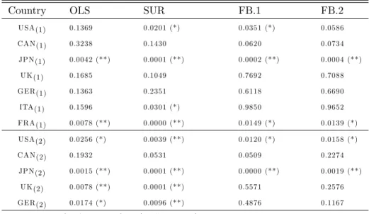
We perform the Wald test for the G-7 countries based on two di¤erent types of time series. The …rst one is the usual time series suggested by the literature (e.g., Ghosh, 1995), in which the Wald test is conducted from a seasonally adjusted quarterly data (at annual rates), expressed in 2000 local currency, converted in per capita real terms, by dividing it by the implicit GDP de‡ator and the population. In order to compute common shocks among the considered countries, we also convert all series to 2000 U.S. dollars. In the second approach, however, data is not expressed in per capita terms and is converted to U.S. dollars by using a
2 3The Wald test can b e im plem ented for several values of the world interest rate (r). However, the results are alm ost the sam e for
proper exchange rate time series, due to the fact that the global shocks must be computed from a proper set of scaled and comparable time series. Since both methodologies lead to very similar results, we next present the results only for the later approach, based on di¤erent estimation procedures: OLS, SUR, FB.1 and FB.2 (see tables 13 and 14 in appendix for further details).24
The …rst estimator is merely OLS equation-by-equation, ignoring possible crossed e¤ects among countries. The second approach, SUR, is just a feasible GLS estimator applied to the considered system of equations and, as already mentioned, might improve the e¢ciency when compared to the OLS method and, thus, the covariance matrix of a SUR estimation could result in a rejection of the model previously accepted in the OLS framework. The last estimators, FB.1 and FB.2, are based on a two-way random error decomposition procedure of Fuller & Battese (1974), in which the residual term is decomposed into individual e¤ects, common shocks, and idiosyncratic terms, i.e., "i;t = vi+et+ i;t. The only di¤erence between these two estimators is that FB.1 assumes a unique global shocket for the whole system of equations, whereas, FB.2 considers a common shock eCA
t for the CAt system of equations, and a di¤erent shock eDZt for the Zt equations.
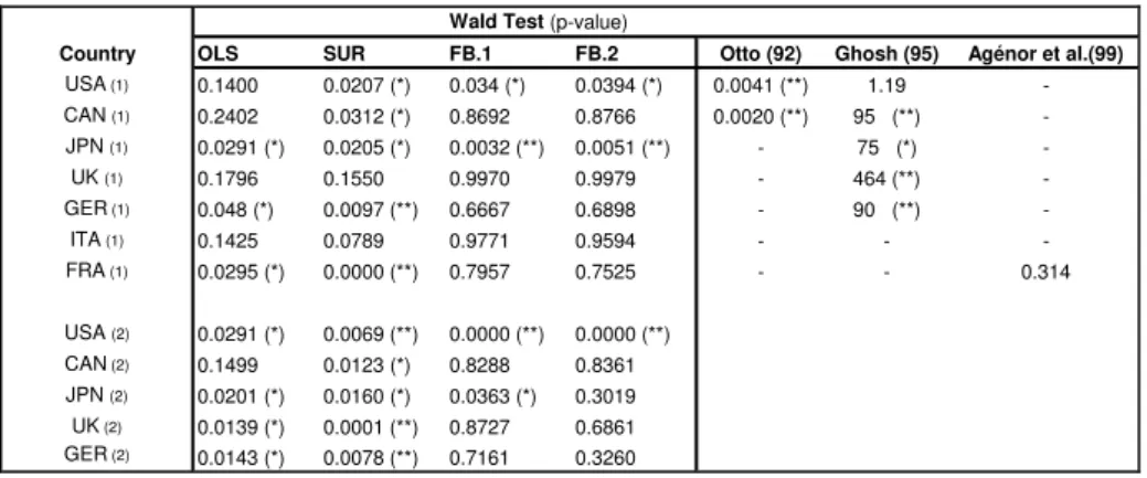
A comparison of these results with the empirical evidence found in the literature is presented in Table 9: Otto (1992) rejects the model for the USA and Canada, Ghosh (1995) rejects the model for Canada, Japan, the UK and Germany, but does not reject it for the USA, and Agénor et al. (1999) do not reject it for France.
Table 9- Comparison with the literature
Wald Test(p-value)
Country OLS SUR FB.1 FB.2 Otto (92) Ghosh (95) Agénor et al.(99)
USA (1) 0.1400 0.0207 (*) 0.034 (*) 0.0394 (*) 0.0041 (**) 1.19 -CAN(1) 0.2402 0.0312 (*) 0.8692 0.8766 0.0020 (**) 95 (**) -JPN(1) 0.0291 (*) 0.0205 (*) 0.0032 (**) 0.0051 (**) - 75 (*) -UK(1) 0.1796 0.1550 0.9970 0.9979 - 464 (**) -GER (1) 0.048 (*) 0.0097 (**) 0.6667 0.6898 - 90 (**) -ITA (1) 0.1425 0.0789 0.9771 0.9594 - - -FRA (1) 0.0295 (*) 0.0000 (**) 0.7957 0.7525 - - 0.314 USA(2) 0.0291 (*) 0.0069 (**) 0.0000 (**) 0.0000 (**)
CAN (2) 0.1499 0.0123 (*) 0.8288 0.8361 JPN(2) 0.0201 (*) 0.0160 (*) 0.0363 (*) 0.3019 UK (2) 0.0139 (*) 0.0001 (**) 0.8727 0.6861 GER (2) 0.0143 (*) 0.0078 (**) 0.7161 0.3260
Notes: Ghosh (1995) presents chi-squared values; USA(1) indicates sample 1
and USA(2) means sample 2; (**) means rejection at 1% level, and (*) at 5% level.
First of all, note that the SUR estimator generally over rejects the model in comparison to OLS.25
However, recall from Proposition 1 that a fair analysis of Table 9 should only consider countries in which
2 4EViews 5.1 was used to obtain the OLS and SUR estim ators, whereas a code in R was develop ed for the FB estim ators, which
could alternatively b e com puted in SAS.
2 5An im p ortant rem ark is provided by Ghosh and Ostry (1995), which argue that the non-rejection of the m odel for a given country
can occur b ecause of the m agnitude of the standard deviations in the coe¢ cients of the VAR. High values for the standard errors could


![Table 6 - Vector K = [ ; ] for UK](https://thumb-eu.123doks.com/thumbv2/123dok_br/15641313.111069/26.892.531.696.259.434/table-vector-k-for-uk.webp)