A Consumption CAPM with a Reference Level
∗Ren´e Garcia
CIREQ, CIRANO and Universit´e de Montr´eal ´
Eric Renault
CIREQ, CIRANO and University of North Carolina at Chapel Hill Andrei Semenov
York University
First version December 2002, This version September 2004
Abstract
We study an intertemporal asset pricing model in which a representative consumer maximizes expected utility derived from both the ratio of his consumption to some reference level and this level itself. If the reference consumption level is assumed to be determined by past consumption levels, the model generalizes the usual habit formation specifications. When the reference level growth rate is made dependent on the market portfolio return and on past consumption growth, the model mixes a consumption CAPM with habit formation together with the CAPM. It therefore provides, in an expected utility framework, a generalization of the non-expected recursive utility model of Epstein and Zin (1989). When we estimate this specification with aggregate per capita consumption, we obtain economically plausible values of the preference parameters, in contrast with the habit formation or the Epstein-Zin cases taken separately. All tests performed with various preference specifications confirm that the reference level enters significantly in the pricing kernel.
JEL classification: G12
Keywords: elasticity of intertemporal substitution, relative risk aversion, habit for-mation, recursive utility, reference level
1
Introduction
The canonical consumption-based capital asset pricing model (CCAPM) where a repre-sentative agent maximizes his expected time-separable utility over uncertain streams of consumption is the workhorse of financial economists. It allows to understand intuitively the marginal utility trade-offs between different time periods or states of nature given some specification of the agent preferences. However, when per capita consumption enters a power utility function, the model delivers gross inconsistencies with the observed asset returns, whether the empirical assessment is based on calibration or on formal estimation. This resilient empirical misfit has triggered, over the last two decades, a long series of attempts to modify the basic model in order to achieve empirical success.
Among the various solutions to the empirical puzzles, enrichments of preferences figure prominently.1 A contribution of our paper is precisely to bring together and generalize three
preference-based approaches that are recognized as the main contenders to explain asset price behavior: a consumption-based solution with habit formation proposed by Campbell and Cochrane (1999); the recursive utility framework of Epstein and Zin (1989) and the prospect-theory alternative specification of utility recently introduced by Barberis, Huang and Santos (2001). A unified way to consider these three a priori different solutions is to realize that in each case a state variable is added to consumption in the utility function of the agent. In habit formation models, an investor derives utility not from the absolute level of consumption but from its level relative to a benchmark which is related to past consumption.2 When this reference level depends on past aggregate per capita consumption, the catching up with the Joneses specification of Abel (1990), or on current per capita consumption, the keeping up with the Joneses of Abel (1999)3, it captures the idea that
the individual wants to maintain his relative status in the economy. In Epstein and Zin (1989), the agent mixes his current consumption with the expected future level of utility to assess his current utility. The solution to this recursive problem introduces the return on the market portfolio in the stochastic discount factor (SDF) which prices assets. Bakshi and Chen (1996) arrives at a similar SDF in a standard expected utility framework by introducing absolute or relative wealth besides consumption in the utility function. Again, the idea of a relative social standing is present in this specification. Finally, a similar idea
1We leave aside approaches that have questioned the representative agent paradigm by introducing in-dividual heterogeneity and estimating the model with microeconomic data. For an overall assessment of the generalizations of the basic asset pricing model with a representative agent, see the excellent surveys of Campbell (2002), Cochrane and Hansen (1992) and Kocherlakota (1996).
2See among others Abel (1990, 1996), Campbell and Cochrane (1999), Constantinides (1990), Ferson and Constantinides (1991), Heaton (1995), and Sundaresan (1989).
is found in Barberis, Huang and Santos (2001), where investors derive utility not only from consumption but also from fluctuations in the value of financial wealth. Their model is influenced both by prospect theory and experimental evidence since the agents are loss averse and the degree of their loss aversion depends on prior investment performance.
In this paper we propose a pure consumption-based model which encompasses the three models just described and offers new specifications. In our model, the state variable is an exogenous reference level of consumptionSt.We start by maintaining that the agent derives
utility not only from the level of consumption relative to this benchmark, as in the external habit formation literature, but also from the absolute value of this reference level, that is
U(Ct
St, St) in ratio form orU(Ct−St, St) in difference form. From a behavioral point of view
it seems restrictive to judge utility only in relative terms, since the state of the economy, captured by St,should also influence the overall satisfaction of the agent. Even if an agent
does not fare as well in a boom as the rest of the economy, he might still be happier just because the overall consumption is higher. This specification will allow us to test formally if the absolute level of per capita consumption is important per itself for pricing assets, over and above consumption relative to the reference level as it is specified in the habit formation model of Constantinides (1990) or Campbell and Cochrane (1999).
The empirical success of the latter habit formation model comes from a utility func-tion with a slow-moving habit and from the nonlinear dynamics imposed on the surplus consumption with respect to the habit. A second contribution of our paper is the statisti-cal model proposed to identify the reference level and its dynamics. While Campbell and Cochrane (1999) model consumption growth as an i.i.d. lognormal process and specify a dynamic model with persistence and conditional heteroskedasticity for the surplus consump-tion, we focus directly on the dynamics of the reference level interpreted as a predictable component of consumption growth. Even though this predictable component is hard to detect in consumption data, it is of utmost importance to explain asset prices, as recently emphasized by Alvarez and Jermann (2002) and Bansal and Yaron (2002).
To keep the model purely consumption-based, we constrain the future values of the reference level through an equality in expectations,Et[St+h] =Et[Ct+h],for allh≥0,where
C will typically refer to aggregate per capita consumption or to the average consumption of a reference group. However, this constraint does not force the consumption reference level to depend solely on consumption.4 It can be a function of other variables in the information
set such as wealth (value of the market portfolio) and we then recover a specification similar to Bakshi and Chen (1996).5The novelty of our approach is apparent when the growth rate
4When the reference level of consumption is identified with the recent past and current aggregate per capita consumptionC, this specification is in fact a general version of the power utility formulation of Abel (1990), which was recently used in a saving and growth model by Carroll, Overland, and Weil (2000).
of the reference level, the predictable part of aggregate per capita consumption growth, is made a function of both past consumption growth and the return of the market portfolio. We obtain in this case a stochastic discount factor (SDF) which embeds the usual habit formation approach together with the so-called Kreps-Porteus specification of the recursive framework of Epstein and Zin (1989). It should be noted that we then obtain a separation between the attitude towards risk and intertemporal substitution even though the agent maximizes expected time-separable utility. Indeed, this separation is generally associated with the non-expected utility framework of Epstein and Zin (1989) where the agent combines his current consumption with expected future utility in a recursive way.
Saying that the future levels of St are equal in expectation to the future levels of
ag-gregate consumption means thatSt represents the permanent component of consumption.
Allowing St to depend on variables other than consumption is suggested by the results
of Alvarez and Jermann (2002) who show that the size of the permanent component in consumption obtained from consumption data alone is much lower than the size of the permanent component of pricing kernels. Therefore, they recommend that in asset pric-ing models preferences should be such as to magnify the size of the permanent component in consumption. When the reference level is made a function of the value of the market portfolio, another permanent component is added to the pricing kernel. In the latter for-mulation, the consumption wealth ratio will enter the pricing kernel. Lettau and Ludvigson (2001) have emphasized the prominent role played by the log consumption-wealth ratio as a conditioning variable for improving the performance of unconditional specifications.
Another important feature of our approach is that the dynamics specified for the growth rate of the reference level adds a moment condition to the set of asset pricing Euler equations. This additional condition relates the growth rate of log consumption to the variables deemed to characterize the growth rate of the log reference level.6 The estimation of this linear
equation delivers an estimated value for the growth rate of the reference level which is used in the asset pricing equations. The estimation of the linear equation and the asset pricing Euler conditions can still be carried out jointly, imposing cross-equation restrictions which improves efficiency of the estimates of preference parameters. Recently, Neely, Roy, and Whiteman (2001) have addressed the issue of near nonidentification of the risk aversion
level of wealth in the economy, while in prospect theory, the utility function is kinked at a reference point which is close to the current level of wealth. Barberis, Huang and Santos (2001) extend prospect theory to make agents less risk averse when their wealth has risen in the recent past. In the last two papers, wealth plays a similar role than reference consumption in habit formation models. While a volatile return on wealth makes the SDF more volatile, and therefore better suited to explain the historical equity premium, it appears as a solution which raises another puzzle. It is hard to reconcile the smoothness of consumption with the volatility of wealth given that consumption and wealth are linked by the intertemporal budget constraint.
parameter in the intertemporal consumption capital asset pricing model. They conclude that imposing natural identifying restrictions yields stable estimates of the parameters.
We follow this approach to estimate several generalized versions of the habit formation models. In ratio specifications, habit may depend on one lag of consumption or respond gradually to changes in consumption. In both cases, we find some support for the presence of the reference level per itself in the utility function, but with estimates of the time discount parameter always greater than one. We also test the specification in difference proposed by Campbell and Cochrane (1999). Contrary to the ratio models, we find strong support for the hypothesis that the absolute value of the reference level enters the utility function.
If we assume that the reference level growth rate is a function of the return on the market portfolio, our model of expected utility yields a SDF which is isomorphic in its pricing implications to the Epstein and Zin (1989, 1991) pricing kernel. A striking feature of the comparison between the Epstein and Zin (1989, 1991) non-expected utility model and our expected utility model with a reference level is that the measures of risk aversion differ while the elasticity of intertemporal substitution remains the same in the two models. We explore in detail this difference in the interpretation of the risk aversion parameter in Garcia, Renault, and Semenov (2002). When we estimate this specification of our model which is observationally equivalent to the Epstein and Zin (1991) specification, we obtain a negative point estimate of the elasticity of intertemporal substitution but not significantly different from zero. Finally, when we allow the reference level growth rate to be determined both by past consumption growth and by the return on the market portfolio, we obtain a SDF which incorporates habit formation in a Epstein-Zin-like SDF. With this specification, we obtain precise and reasonable estimates of the coefficient of relative risk aversion (around 1), of the elasticity of intertemporal substitution (0.86), and of the time discount factor (0.9988).
Our reference level model can accommodate specifications in which the investor expresses disappointment or loss aversion whenever his consumption falls under the reference level. Our results show that for consumption above habit, the most plausible assumption is that the representative consumer derives utility from both consumption relative to habit and the absolute level of habit. As consumption declines towards the benchmark level, we cannot reject the assumption that the conventional time- and state-separable utility model describes well the agent’s preferences. When we test a model of loss aversion similar to Barberis, Huang, and Santos (2001), we confirm the importance of the absolute value of the reference level in the utility function. Therefore, we are led to conclude that our utility specification not only opens new avenues for modeling the SDF but is robust to existing extensions of the standard CCAPM model.
stochastic prices of consumption risks and adds flexibility to the standard CCAPM through the risk aversion specification.7 By allowing attitudes towards risk to reflect the information
set used for consumption and savings choices, risk aversion is no longer fixed, but contingent upon the state of the world.8 The same individual may be a risk-lover over certain states of the world and risk averse over others, adjusting his tolerance to risk according to the characteristics of the problem that he faces. Such shifts in attitudes could be related to numerous factors. Bakshi and Chen (1996) and St-Amour (1993), for example, allow for wealth-dependent attitudes towards risk, when the equilibrium relative risk aversion is a decreasing function of the individual’s wealth, thus implying countercyclicality of risk aver-sion. In Campbell and Cochrane (1999), Constantinides (1990), and Sundaresan (1989), who introduce time-varying prices of risk through habit formation, relative risk aversion in-creases as consumption declines towards habit and, therefore, also displays a countercyclical pattern.
Our model may be given an alternative interpretation. The representative agent can be thought as a portfolio manager whose performance is evaluated in terms of a benchmark as it is the case in practice.9 The idea of a reference level determining the utility of the investor is related to an older literature. Porter (1974), Fishburn (1977), and Holthausen (1981) present a risk-return model in which risk is associated with outcomes below some specified target level and return is associated with outcomes above the target. A decision maker may display different preferences for outcomes above and below the target outcome. They show congruence between that model and a specific form of expected utility function. Our model may be viewed as a particular extension to a dynamic setting of that risk-return approach, when the reference level is seen as a target.
The rest of the paper is organized as follows. In Section 2, we discuss the major features of the model in which a consumer derives utility from consumption relative to some reference consumption level as well as from this level itself. In particular we propose various dynamics for the evolution over time of the reference level which depend on the information set used by the agent to forecast the state of the economy. Section 3 examines the empirical implications of the proposed utility function under alternative specifications of the reference level generating process and assesses the contribution of the model towards explaining asset returns in US monthly data. Conclusions are presented in Section 4.
7One can include in this line of research Bakshi and Chen (1996), Campbell and Cochrane (1999), Chou, Engle, and Kane (1992), Constantinides (1990), Gordon and St-Amour (1998a, 1998b), Harvey (1991), Mark (1988), McCurdy and Morgan (1991), Melino and Yang (2003), St-Amour (1993), and Sundaresan (1989).
8In the standard power utility model, the SDF is just consumption growth raised to the power
−γ and,
thus, one needs a large value ofγ to get a volatile pricing kernel. The state dependent risk aversion implies that consumption shocks generate larger unanticipated fluctuations in marginal utility than under fixed preferences and, therefore, one can instead get a volatile SDF from a volatile relative risk aversion.
2
An Expected Utility Model with a Reference Consumption Level
We generalize the standard time-separable power utility function by assuming that each consumer derives utility from consumption relative to some reference consumption level as well as from this level itself:
ut=
Ct
St 1−γ
St1−ϕ
sign(1−γ)sign(1−ϕ), (1)
whereγ is the curvature parameter for relative consumption,Ctis current consumption,St
is a time-varying reference consumption level, and the parameterϕ controls the curvature of utility over this benchmark level. We adopt the convention that sign(x) = x if x ≥ 0 and sign(x) = −x if x < 0. If ϕ = γ, we get the standard time-separable power utility function (the reference consumption level plays no role in asset pricing). With ϕ= 1, we obtain a preference specification where the ratio of the agent’s consumption to the reference consumption level is all that matters, as in habit formation models. If ϕ6=γ and ϕ 6= 1, then the agent takes into account both the ratio of his consumption to the reference level and this level itself when choosing how much to consume. Then, when maximizing expected utility over an infinite horizon, the agent assesses:
Vt= [sign(1−γ)sign(1−ϕ)]−1
X∞
h=oδ hE
t
"
Ct+h
St+h
1−γ
St1+−hϕ
#
. (2)
We consider that the reference level St is external to the agent andEt denotes a
con-ditional expectation given the information at time t. At the most general level in a rep-resentative agent framework, this benchmark consumption provides a way to extend the intertemporal choice of consumption without uncertainty to risky consumption streams. When no uncertainty prevails, the future sequence of the reference level at time t, St+h,
h≥0,coincides with the optimal future aggregate consumption values:
St+h=Ct+h identically forh≥0. (3)
In a risky environment, we just generalize condition (??) in terms of conditional expec-tations:
Et[St+h] =Et[Ct+h] for all h≥0. (4)
Therefore, we can interpret St+h as the reference level the agent has in mind at time t
when deciding his risk-taking behavior. In the latter case, some macroeconomic variables which belong to the agent’s information set at time (t+h) may affect the assessment of the reference levelSt+h. Even with this constraint on the reference level, the utility specification
consumption reference level with respect to the existing asset pricing models and possible extensions of these models, we need to establish how the presence of this benchmark will change the intertemporal consumption trade-offs and the risk premia.
Since the reference level is considered external, the marginal utility of consumption is given by
∂ut
∂Ct
=Ct−γSγ
−ϕ
t . (5)
Then, when maximizing his expected utility over an infinite horizon, the investor will choose an optimal consumption profile which will satisfy the following Euler equations:
Et
"
δ
Ct+1
Ct
−γ
St+1
St
γ−ϕ
Ri,t+1 #
= 1, i= 1, ..., I, (6)
where I is the number of assets considered and Ri,t+1 is the gross return of asset i from
t to t+ 1. Expectations in (??) are taken conditionally on information available to the individual in period tand Rit is the gross return on asseti. The SDF is then
Mt+1 =δ
Ct+1
Ct
−γ
St+1
St
γ−ϕ
. (7)
To discuss the implications of asset pricing models, it is common to assume joint condi-tional lognormality and homoscedasticity of the consumption growth rate and asset returns, since we obtain loglinear relations for asset returns. With our utility model, the risk-free rate will be determined by the following equation:
rf,t+1 =−logδ+γEt[∆ct+1]−
1 2γ
2σ2
c
−(γ−ϕ)Et[∆st+1]−
1
2(γ−ϕ)
2σ2
s+γ(γ−ϕ)σcs, (8)
whereas the risk premium on any asset iwill be given by:
Et[ri,t+1−rf,t+1] =−
1 2σ
2
i +γσic−(γ−ϕ)σis, (9)
where ∆ct+1 is the log of the consumption growth rate, ∆st+1 is the log of the reference
consumption level growth rate, ri,t+1 is the log of the simple gross return on asset i, and
σxy denotes generically the unconditional covariance of innovations.
The first three terms on the hand side of (??) and the first two terms on the right-hand side of (??) are the same as for a time-separable power utility function of consumption alone. Thus, utility function (??) can help to explain the risk-free rate puzzle if the term
−(γ−ϕ)Et[∆st+1]− 12(γ−ϕ)2σ2s + γ(γ−ϕ)σcs is negative and the equity premium
puzzle if the term −(γ−ϕ)σis is positive. Therefore, the position of γ with respect toϕ
and the innovations in consumption growth and in asset returns are key in solving the two puzzles.
Another important dimension over which the resolution of the puzzles is discussed is the disentangling of risk aversion and intertemporal substitution. The standard consumption CAPM model with power utility imposes a functional restriction which is not sustainable theoretically nor supported empirically. For our model, we can study this separation by writing the expected return equation, always under the same joint conditional lognormality and homoscedasticity of the consumption growth rate and asset returns:
Et[ri,t+1] =−logδ+γEt[∆ct+1]−
1 2γ
2σ2
c−(γ−ϕ)Et[∆st+1]
−1
2(γ−ϕ)
2
σ2s+γ(γ−ϕ)σcs−
1 2σ
2
i +γσic−(γ−ϕ)σis. (10)
To study intertemporal substitution in a simplified framework, let us assume that all quantities are now deterministic so we can ignore the expectation operators. With the standard power utility function under this assumption, equation (??) reduces to
rt+1=−logδ+γ∆ct+1−
1 2γ
2σ2
c, (11)
which implies σ = γ1 = ∂∆ct+1
∂rt+1 .From (??), it follows that when the agent’s preferences are
of the form (??), the intertemporal elasticity of consumption is
σ = ∂∆ct+1
∂rt+1
= 1 + (γ−ϕ)
∂△st+1
∂rt+1
γ , (12)
where ∂△st+1
∂rt+1 can be interpreted as the elasticity of the reference level with respect to the
interest rate.10 The latter equation implies that the elasticity of intertemporal substitution differs from the inverse of the RRA coefficient if (γ−ϕ)∂△st+1
∂rt+1 6= 0. In our external
reference level setting, it will therefore be important to distinguish the specifications where this level depends on past variables, in which case the disentangling will not occur, from the ones where it depends on contemporary variables and allows to differentiateσ from the inverse ofγ.11We will therefore separate our analysis of the various models for the reference level into two sections. In the first one we will consider that the reference level depends only on past variables as it is often the case in the habit formation literature. In the second we will allow the reference level to be determined by contemporaneous variables.
10As we can see from equations (
??) and (??), since the terms ∂△st+1
∂rt+1 and σis have the same sign, if
utility model (??) generates an equity premium which is larger than that produced by the basic power utility model, it also generates an elasticity of intertemporal substitution which is less than the inverse of the RRA coefficient.
2.1 Reference Level Determined by Past Variables
In this subsection we will model the reference level strictly as a function of past variables, mainly lagged aggregate per capita consumption. This will allow us to make the link with the habit formation literature and discuss how our model has the potential to extend it. We will also discuss the issue of persistence of the reference level.
2.1.1 Modeling of the Reference Level
An approach commonly used in the literature consists in assuming that the reference con-sumption level, St+1, is an expectation of consumption Ct+1 taken conditionally on past
consumption levels, that isSt+1 =E[Ct+1|Ct, Ct−1, ...].12 According to this approach, the
time-varying habit can be specified either as an internal habit (habit depends on agent’s own consumption) (Constantinides (1990), Sundaresan (1989)) or as an external habit (the indi-vidual’s reference consumption level depends on aggregate consumption, which is assumed to be unaffected by any one agent’s consumption decisions, rather than on the history of individual’s own consumption) (Abel, 1990, 1996, Campbell and Cochrane, 1999).
Let us start with the case where St =Cαt−1, as in Abel (1990). As already mentioned,
the ratio habit-formation model or the catching up with the Joneses are special cases of (??) when ϕ= 1.The utility function is in this case:
ut=
Ct
Cαt−1 1−γ
1−γ (13)
which, with α= 0,gives the standard time-separable model and, with α= 1,the catching up with the Joneses model. In the latter case, only relative consumption matters to the consumer. Recently, Carroll, Overland, and Weil (2000) and Fuhrer (2000) have argued that one need not impose the constraint that α has to be 0 or 1.For values of α between 0 and 1, both the absolute and relative consumption levels are important to the consumer. The way we have rewritten the utility function lends itself to a different interpretation. Let us suppose that actual consumption never deviates from the reference level. In this case there is no consumption risk and the consumer needs just decide how to intertemporally substitute consumption over time. The exponent of the reference level is then quite naturally
ρ= 1−ϕ, with the elasticity of intertemporal substitutionσ = 1/(1−ρ).Of course, there is consumption risk and the consumer reacts to it trough the curvature parameterγ which measures risk aversion.
Even though a number of papers have assumed that habit depends on only one lag of consumption, an alternative view is that the habit level responds only gradually to changes
in consumption.13 Carroll, Overland, and Weil (2000), Constantinides (1990), and Fuhrer
(2000), for example, assume that the benchmark level evolves according to the adaptive expectations hypothesis, which postulates that the change in expectations, St+1 −St, is
equal to a proportionλof last period’s error in expectations,Ct−St:
St+1−St=λ(Ct−St), 06λ61 (14)
or, equivalently,
St+1 =λCt+ (1−λ)St. (15)
We consider the unrestricted form of (??):
St+1 =a+λCt+ (1−λ)St. (16)
After repeated substitution, we finally obtain:
St+1 =
a λ+λ
∞ X
i=0
(1−λ)iCt−i (17)
which means that the habit stock is a weighted average of past consumption flows with the weightsλ(1−λ)i declining geometrically with time.
Since the subsistence level,St+1, is assumed to be an expectation of consumption taken
conditionally on past consumption levels, we can rewrite (??) as
Ct+1=
a λ+λ
∞ X
i=0
(1−λ)iCt−i+εt+1, (18)
where εt+1 is an innovation in Ct+1. Estimating this equation allows us to recover the
parameters aand λand therefore obtain an estimate of the reference level.
2.1.2 Persistence of the Reference Level
The persistence of the reference level formation process is an important issue for consumption-based asset pricing models. Alvarez and Jermann (2002) derive a lower bound for the size of the permanent component of asset pricing kernels and find that it is very large. They also show that in the many instances where the pricing kernel is a function of consumption, in-novations to consumption must have permanent effects. When Alvarez and Jermann (2002) measure the size of the permanent component of consumption using only consumption data, they find it is well lower than the size of the permanent component of pricing kernels. They suggest that in a representative agent asset pricing framework the specification of prefer-ences should magnify the permanent component in consumption. The reference level in
our utility function offers a way to introduce variables which, along with consumption, will contribute to amplify the permanent component of the asset pricing kernel. We will ex-plore these possibilities in the next section where we will most notably look at the link between the reference level and the return on the market portfolio. Additionally, adding contemporaneous variables will allow to disentangle risk aversion from intertemporal sub-stitution, whereas this disentangling could not occur when the reference level depended on past aggregate consumption, as explained in the introduction to the section
2.2 Reference Level Determined by Contemporaneous State Variables
A more general approach to modeling the subsistence level formation process is to assume that an agent can take into account not only the information available to him at timet, but also some information available at timet+1, when he forms his reference consumption level,
St+1. Abel (1999) and Cochrane (2001), for example, suppose that the agent’s benchmark
level depends on current period aggregate consumption. Campbell and Cochrane (1999) also make their habit a contemporaneous variable.
According to (??), the reference consumption level growth rate is all we need to know about the reference level for asset pricing. We first motivate by an economic argument why the reference level growth rate should be made a function of the return of the market portfolio. We then present a general framework which allows other contemporaneous or past state variables to explain the reference level growth rate. We further show how to nest in this framework both the Epstein and Zin (1989, 1991) pricing kernel and the power utility model of Campbell and Cochrane (1999) with a slow-moving external habit.
2.2.1 Modeling the Growth Rate of the Reference Consumption Level
The SDF defined in (??) implies that the reference level must produce conditional expecta-tions which not only are constrained by (??) but also are consistent with asset prices. Let us consider first the market portfolio pricing condition. If we denote by RM,t+1 the gross
return on the market portfolio observed at time (t+ 1), we get
Et
"
δ
Ct+1
Ct
−γ
St+1
St
γ−ϕ
RM,t+1 #
= 1. (19)
investment performance. To make even more explicit this tight relationship between the reference level and investment performance as measured by the market return, we will refer to a loglinearization of conditional moment restrictions (??) and (??) (see Epstein and Zin (1991) and Campbell (1993) for similar interpretations based on a loglinearization of the Euler equations). Conditional expectations are computed as if the vector
(∆ct+1,∆st+1, rM,t+1) =
log
Ct+1
Ct
, log
St+1
St
, logRM,t+1
(20)
were jointly normal and homoscedastic given the information available at timet. Conditions (??) and (??) at horizon 1 become:
Et[∆ct+1]−Et[∆st+1] =κ1, (21)
−γEt[∆ct+1] + (γ−ϕ)Et[∆st+1] +Et[rM,t+1] =κ2 (22)
for some constants κ1and κ2. Equivalently, these two restrictions say that both [∆st+1−
∆ct+1] and [∆st+1−ϕ1rM,t+1] must be unpredictable at timet. The Epstein and Zin (1989)
pricing model is in fact observationally equivalent to the particular case of our CCAPM with reference level where [∆st+1−ϕ1rM,t+1] is not only unpredictable but constant:
∆st+1=
1
ϕrM,t+1+κ, (23)
for some constantκ. In other words, we consider the particular case where the benchmark growth rate of consumption is loglinearly determined by the current value of the market return, with a slope parameter equal to the elasticity of intertemporal substitution. Note that this is in accordance with the portfolio separation property generally implied by ho-motheticity of preferences (see Epstein and Zin, 1989), whereby optimal consumption is determined in a second stage, after the portfolio choice has been made.
An interesting generalization is to relate the log of reference level growth to past period consumption growth, as we did in the previous section for habit formation models, and the current period return on the market portfolio in the following way:
△st+1 =a0+
n
X
i=1
ai· △ct+1−i+b·rM,t+1.14 (24)
Condition (??) is consistent with a model where consumption growth is equal to the reference level growth rate plus a constant and noise:
∆ct+1=κ1+ ∆st+1+εt+1, (25)
where εt+1 is an innovation in △ct+1 with Et(εt+1) = 0 andEt[∆st+1εt+1] = 0. It follows
that the log of consumption growth may be described by an affine regression
△ct+1 =a0+κ1+
n
X
i=1
ai· △ct+1−i+b·rM,t+1+εt+1, (26)
withEt[rM,t+1εt+1] = 015.From (??),
St+1
St
=A
n
Y
i=1
Ct+1−i
Ct−i
ai
(RM,t+1)b, (27)
whereA≡exp(a0+κ1).
Under the above assumptions, the SDF (??) becomes
Mt+1=δ∗ C
t+1
Ct
−γ n Y
i=1 C
t+1−i
Ct−i
ai(γ−ϕ)
(RM,t+1)b(γ−ϕ), (28)
where δ∗ ≡ δAγ−ϕ. This specification allows to separate risk aversion from intertemporal
substitution, since σ= 1+b(γγ−ϕ). Therefore, we may rewrite (??) as
Mt+1=δ∗
Ct+1
Ct
−γ n Y
i=1
Ct+1−i
Ct−i
ai(γ−ϕ)
(RM,t+1)κ, (29)
where κ ≡σγ −1, so that testing the null hypothesis H0 :κ = 0 is equivalent to testing
H0:σ = 1γ.
This specification of the SDF is interesting for several reasons. First, when ai = 0
(i= 1, ..., n), the SDF in (??) is isomorphic in its pricing implications to the Epstein and Zin (1989, 1991) pricing kernel for a Kreps and Porteus (1978) certainty equivalent. When
b = 0, the reference level growth depends only on previous period consumption growth, as in the habit formation approach. When neither of these restrictions holds, we have a new asset pricing model which puts together two strands of the literature which evolved in parallel until now.16 This new framework offers a way to test existing models since they are embedded in the general specification. Let us look in more detail at the comparison between the Epstein-Zin SDF obtained under a non-expected recursive utility model and the SDF under expected utility with a reference level.
15This provides identification of the coefficient of returns in the prediction equation of consumption since the imposed equality in expectations between consumption and the reference level which leads to (??) is not sufficient to provide this identification.
2.2.2 Comparison with the Epstein-Zin Stochastic Discount Factor
Under the assumption that ai = 0 (i= 1, ..., n), the SDF in (??) reduces to
Mt+1 =δ∗
Ct+1
Ct
−γ
(RM,t+1)κ. (30)
When γ = 1/σ (i.e. κ= 0), we get the SDF for a standard power utility model. When
γ = 0, the consumption growth rate is irrelevant to the determination of equilibrium asset prices and the market return is sufficient for discounting asset payoffs. In any other case, both the consumption growth rate and the market return are relevant to the determination of equilibrium asset prices.
The Epstein-Zin (1989, 1991) SDF is
Mt+1=µ 1−α
ρ
Ct+1
Ct
1−α ρ (ρ−1)
(RM,t+1) 1−α
ρ −1, (31)
whereρis the parameter reflecting intertemporal substitutability (the elasticity of intertem-poral substitution isψ= 1/(1−ρ)) andα is the risk aversion parameter. Epstein and Zin (1989) interpret α as a measure of risk aversion for comparative purposes with the degree of risk aversion increasing inα.
The observational equivalence between the SDFs (??) and (??) implies thatδ∗ ≡µ1−ρα,
−γ ≡ 1−α
ρ (ρ−1), and σγ −1 ≡ 1
−α
ρ −1. The two last identities put together yield
σ= 1ργ−α = 1/(1−ρ) =ψ, that is the elasticity of intertemporal substitution in model (??) is equivalent to that in the Epstein-Zin non-expected recursive utility specification. In the case of the Epstein-Zin utility function, the elasticity of intertemporal substitution may not be equal to 1, whereas in the case of utility specification (??) any value ofσ is allowed.
Since σ = 1/(1−ρ),γ = (1−α)/(σ−1). It follows that the measure of risk aversion in the Epstein-Zin (1989, 1991) utility specification, α, is equal to 1−γσ+γ. It is easy to see thatα is equal to the RRA coefficient,γ, only ifγ = 1/σ, what corresponds to the case of the standard power utility model.17 Ifγ differs from 1/σ, the parameter α is no longer the RRA coefficient and is equal to the RRA coefficient plus the term 1−γσ.
Several comments are in order. First, the ability of the recursive utility model to dis-entangle risk aversion and intertemporal substitution is questionable. Actually, it is only in the standard expected utility model case, whenσ is the inverse of the risk aversion pa-rameterγ,that α can be interpreted as a risk aversion parameter. Even more problematic is the fact that α becomes negative whenever σ is greater than γ1 + 1.Note that this lack of disentangling manifests itself even without resorting to our interpretation ofγ as a risk
aversion parameter. The natural requirement of a negative exponent for Ct+1
Ct in the SDF
implies that the alleged risk aversion parameter α and σ1 should be on the same side of 1. Second, as soon as σ is greater than γ1, the alleged risk aversion parameter α underes-timates the genuine risk aversion parameter γ. Hence, a relatively high level of elasticity of intertemporal substitution may spuriously indicate a moderate risk aversion. If, as doc-umented by Mehra and Prescott (1985), the model can replicate the equity risk premium only for a high level of risk aversion, sayγ = 20, even a moderate elasticity of substitution, say .8, will dramatically lower the perceived risk aversion in the recursive utility model, i.e.
α= 5.
In our model, risk aversion is defined with respect to the unpredictable discrepancy between actual consumption and the reference level (a quantity independent of the attitude towards risk) and not with respect to the forthcoming level of recursive utility which still mixes attitudes towards risk and intertemporal substitution. Garcia, Renault, and Semenov (2002) develops further the comparison between the two models.
The SDF in (??) yields the following Euler equations:
Et
"
δ∗
Ct+1
Ct
−γ
(RM,t+1)κRi,t+1 #
= 1, i= 1, ..., I.18 (32)
A test of the null hypothesisH0:σ = 0 can be carried out by testing the null hypothesis
H0 :κ=−1 and γ 6= 0. To examine whether σ= 1/γ, we have to test the null hypothesis
H0:κ= 0.
We may rewrite the SDF in (??) as
Mt+1 = δ∗
Ct+1
Ct
−γ
(RM,t+1)b(γ −ϕ)
= δ∗1/θ
C
t+1
Ct
−ϕ!θ
(RM,t+1)−bϕ 1−θ
. (33)
Approximating this geometric average with an arithmetic average yields
Mt+1 =θ δ∗1/θ
Ct+1
Ct
−ϕ!
+ (1−θ) (RM,t+1) −bϕ
. (34)
After substituting this linear approximation into the Euler equations (??), we obtain
1≈θEt
"
δ∗1/θ
Ct+1
Ct
−ϕ
(Ri,t+1) #
+ (1−θ)Et
h
(RM,t+1) −bϕ
(Ri,t+1) i
. (35)
It can be viewed from (??) that, as in the Epstein-Zin utility function case, the riskiness of an asset is measured by means of the covariance of its return with the market portfolio
18Sinceκ=σγ
−1, one may want to estimateσ directly. However, we prefer estimatingκinstead of σ
return (as in the static CAPM) and the covariance of its return with the consumption growth rate (as in the intertemporal CAPM).
Another usual way to illustrate this interpretation is to assume joint lognormality and homoscedasticity of the consumption growth rate and asset returns. Under this assumption, we have
Et[ri,t+1−rf,t+1] =−
1 2σ
2
i +γσic−(γ−ϕ)bσiM =−
1 2σ
2
i +ϕ(θσic+ (1−θ)bσiM). (36)
So, the parameter ϕ can be thought of as a coefficient measuring the contribution of a weighted combination of asset i’s covariance with consumption growth and asset i’s covariance with the market return towards the risk premium on asseti.
Alvarez and Jermann (2002) refer to the recursive preferences of Epstein and Zin (1989) and Weil (1989) as a way to increase the size of the permanent component in the pricing kernel. Our utility specification, through the assumed connection between the reference level and the value of the market portfolio, adds similarly a permanent component to the pricing kernel.
2.2.3 Habit Formation in Difference with a Reference Level
Campbell and Cochrane (1999) interpretation of the reference levelStas an external habit
leads them to specify some nonlinear dynamics consistent with the structural restriction
St ≤ Ct. Actually they specify the surplus consumption Ht = CtC−tSt as a conditionally
lognormal process. In this setting, we can still introduce our reference level principle by considering that the representative consumer derives utility from consumption relative to his reference level as well as from this level itself
ut= C
1−γ
t Sγ
−ϕ
t
sign(1−γ)sign(1−ϕ), (37)
according to (??). However, in order to really nest Campbell and Cochrane (1999) utility model, we must extend this formulation by writing
ut= (CtHt)
1−γ
Stγ−ϕ
sign(1−γ)sign(1−ϕ). (38)
Then, testing H0 : γ = ϕ amounts to testing the particular case of Campbell and
economic model, the optimizing agent considers the product (CtHt) as its optimal control
variable given the external habit level St.Therefore, the resulting SDF is:
Mt+1=δ
Ht+1
Ht
−γ
Ct+1
Ct
−γ
St+1
St
γ−ϕ
. (39)
Another way to understand this formula is to realize that the utility function in (??) can also be written :
ut= (Ct−St)
1−γ
Stγ−ϕ
sign(1−γ)sign(1−ϕ), (40)
and the consumer see the reference level Stas external.
The statistical model proposed by Campbell and Cochrane (1999) is specified in order to make the volatility of the SDF stochastically time-varying with the business cycle pattern. The consumption process is seen as a lognormal random walk19 while the logHt process
has the same standardized innovation but evolves as a heteroscedastic AR(1):
∆ct+1 =g+νt+1, νt+1 i.i.d. N(0, σ2), (41)
ht+1 = (1−φ)h+φht+λ(ht)νt+1.
We use the sensitivity function λ(ht) proposed by Campbell and Cochrane (1999), that
is:
λ(ht) =
( 1
H
q
1−2(ht−h)−1 ifht≤hmax
0 otherwise, (42)
where hmax ≡ h + 12(1−H2) and H = σ q γ
1−φ. By choosing this sensitivity function,
Campbell and Cochrane (1999) had two objectives in mind. The first was to obtain a constant risk-free rate. This restriction is typically relaxed in our more general setting with
γ 6= ϕ, where the absolute value of the reference level plays an independent role in the utility function. The second one was to ensure that the elasticity of the reference level with respect to consumption is zero in the steady state and is a U-shaped function of h around
h=h. This objective is still achieved in our setting.
Besides allowing for a time-varying risk-free interest rate, our setting with γ 6=ϕ disen-tangles the relative risk aversion coefficient and the elasticity of intertemporal substitution, as already emphasized in the Epstein-Zin-like interpretation of our model in the previous section. This disentangling appears important since in the Campbell and Cochrane (1999) model risk aversion (Hγ
t) can become very large in the states of the economy where Ht
approaches zero, that is when consumption comes very close to the external habit. In our
setting, a large risk aversion does not automatically imply a dramatically low level for the elasticity of intertemporal substitution. However, as in Campbell and Cochrane (1999), we make the steady state of the reference level (and in turn the sensitivity function) depend on the preferences only through the risk aversion parameterγ.
Campbell and Cochrane calibrated the parameters in order to assess the model implica-tions for asset pricing. Suppose we wanted to estimate this model and test their specification against the more general SDF (??). We should be able to compute the time series of surplus consumption H and to deduce the time series of the growth rate of the reference level S. For the former, givenγ and a process for consumption growth, we need the parameterφ.In choosing parameters, Campbell and Cochrane match φ to the serial correlation of the log price-dividend ratio. But this measure of persistence is tightly related to the persistence of the market portfolio return since one can always write
logRM,t+1 = ∆ct+1+log(1 +Qt+1)−logQt, (43)
whereRM,t+1 = Pt+1+PtCt+1 andQt+1= CPt+1t+1 denotes the price-dividend ratio for a claim on
aggregate consumption. Therefore, approximately
logRM,t+1 ∼= ∆ct+1+log(Qt+1)−logQt. (44)
When ∆ct+1 is viewed as a white noise (as in Campbell and Cochrane (1999)), the
dynamics of the rate of growth of the price dividend ratio is tightly related to the one of the market return. In other words, plugging into the SDF (??) a rate of growth of the reference level that mimics the price dividend ratio dynamics is very similar in spirit to the Epstein and Zin SDF, as revisited in the previous subsection. In this sense, we can claim that our proposed extension of Campbell and Cochrane (1999) nests the Epstein and Zin (1989) asset pricing model expressed with a habit formation model in difference. Therefore, as with the ratio model in section (??), we maintain habit formation preferences while disentangling risk aversion from intertemporal substitution in a way observationally equivalent to Epstein and Zin (1989).
2.3 Preferences with a Reference Level as a Threshold
Bekaert, Hodrick, and Marshall (1997), Bonomo and Garcia (1993), and Epstein and Zin (2001) explore the asset pricing implications of disappointment aversion. Benartzi and Thaler (1993) also adopt asymmetric preferences over good and bad results, but instead of using an intertemporal asset pricing framework with preferences defined over consumption streams, they start from preferences defined over one-period returns based on Kahneman and Tversky (1979)’s prospect theory of choice. The central idea of prospect theory is that an investor is assumed to derive utility from fluctuations in the value of his financial wealth and to be loss averse over these fluctuations, meaning that he is distinctly more sensitive to reductions in his financial wealth than to increases. Recently, Barberis, Huang, and Santos (2001) have studied asset prices in the context of prospect theory. In their model, investors derive utility both from consumption and changes in the value of their financial wealth. They introduce loss aversion over financial wealth fluctuations and allow the degree of loss aversion to be affected by prior investment performance.
The utility function defined in (??) offers at least two ways to model asymmetric pref-erences. First, we can use the reference consumption level St as a threshold below which
outcomes are penalized in terms of utility. In this generalization of habit formation models, investors will have the following utility function:
ut=
✏ Ct St
✑1−γ1
St1−ϕ−1
1−γ1 ifCt>St
λ ✏
Ct St
✑1−γ2
S1−t ϕ−1
1−γ2 otherwise,
(45)
where λis a disappointment aversion coefficient. The intuition here is that the investor is likely to be disappointed if his consumption is lower than the reference level and, conversely, satisfied otherwise. Note that we maintain the same parameter ϕ above and below the threshold for parsimony reasons even though it is conceivable to have different attitudes towards intertemporal substitution in the two states of the world.
A second type of asymmetry could be built by modeling the threshold level in a fashion similar to Barberis, Huang, and Santos (2001). The reference levelSt in this case could be
assimilated to the value of the market portfolio, while the threshold will be given by the position of the return on the market portfolio with respect to the safe asset return. Such a utility specification yields the following SDF:
Mt+1 =δ
C−γ1
t+1V
ϕ
t+1I[RM,t+1>ztRf,t+1] +λ(zt)C −γ2 t+1V
ϕ t+1
1−I[R
M,t+1>ztRf,t+1]
C−γ1
t VtϕI[RM,t>ztRf,t] +λC −γ2 t Vtϕ
1−I[R
M,t>ztRf,t]
, (46)
whereRM,t+1is the return on the market portfolio,Rf,t+1is the risk-free interest rate,Vt+1
is the value of market portfolio, andI[R
M,t+1>ztRf,t+1] is the indicator function, which takes
losses. The larger the prior losses, the more painful subsequent losses will be. Our goal will be to estimate such models by the generalized method of moments to assess the presence of such preferences in the data, as opposed to the calibration exercise of Barberis, Huang, and Santos (2001).
3
Empirical Results for Alternative Models of the Reference Level
In this section, we estimate the models described in Section 2 using US monthly data. After a brief description of data construction, we discuss the estimation procedure in light of the identification issues surrounding the preference parameters. We then start by providing the empirical results corresponding to the conventional time- and state-separable preferences. This will provide a basis with which to compare the richer specifications offered by the three types of models with a reference level discussed in section 2. First, we estimate models for the augmented habit formation approach, where the absolute value of the reference level enters in the utility function along with relative consumption. Second, we consider several specifications where the market portfolio return enters in the determination of the reference level growth rate. We estimate models which embed two well-known models: the Campbell and Cochrane (1999) habit formation model and the Epstein and Zin (1989, 1991) non-expected recursive utility model. For the former case, instead of calibrating the model, we estimate and test the model in a GMM framework keeping the original specification of the consumption surplus dynamics. For the latter, we estimate a utility specification where the reference consumption level growth rate is assumed to depend on the previous period consumption growth rates and the return on the market portfolio. As the Epstein-Zin model is seen to be a mixture of the CAPM and the CCAPM models, this generalized specification can be described as a combination of the CAPM with a habit formation CCAPM model. Finally, we estimate models of asymmetric preferences, where the investor draws different utilities above and below the reference level or some function of it. Most notably, we estimate a model of loss aversion very similar in spirit to the model of Barberis, Huang, and Santos (2001), thereby providing a useful complement to their calibration exercise.
3.1 Data and Estimation Issues
3.1.1 Consumption and Returns Data
The measure of real aggregate consumption used in this paper is the personal consumption expenditures (in constant 1987 dollars) on nondurables and services (NDS) taken from the United States National Income and Product Accounts.20 Monthly per capita consumption
is obtained by dividing the real aggregate consumption by the total population, including armed forces overseas.21
The nominal, monthly risk-free rate of interest is the one-month Treasury bill return from the Center for Research in Security Prices (CRSP) of the University of Chicago. The real risk-free rate is calculated as the nominal risk-free rate, divided by the one-month inflation rate, based on the deflator defined for NDS consumption. As a proxy for the nominal, monthly market return, we take the value-weighted aggregate nominal, monthly return (capital gain plus dividends) on all stocks listed on the NYSE and AMEX, obtained from CRSP. The real, monthly market return is calculated as the nominal market return, divided by the one-month inflation rate. The size portfolios are also obtained from CRSP and are formed with all stocks listed on the NYSE and AMEX.
3.1.2 Estimation and Identification Issues
An iterated GMM approach is used to test Euler equations and estimate model parameters. For each preference specification the Euler equations for the excess market return and the real risk-free interest rate are estimated jointly together with the process describing the evolution of the reference level. Our typical set of equations will be:
Et
"
δ
Ct+1
Ct
−γ
St+1
St
γ−ϕ
Rf,t+1 #
= 1, (47)
Et
"C
t+1
Ct
−γ
St+1
St
γ−ϕ
(RM,t+1−Rf,t+1) #
= 0.
△st+1=a+xt+1b
where st+1 = logSt+1 and xt+1 represents a vector of variables, current and past, deemed
to forecast the growth of the reference level. Using condition (??) at horizon 1 one can write an equation in terms of aggregate consumption growth similar to (??):
△ct+1 =a1+xt+1b+εt+1 (48)
Note that we do not keep the upper bar over aggregate consumption since it is the same as the consumption of the representative agent.
It is by now well established22 that asymptotic normality is often a poor approximation for the sampling distributions of the GMM estimators. These distributions can be skewed and have fat tails. Tests of overidentifying restrictions can exhibit important size distortions.
21CITIBASE, mnemonic POP.
Stock and Wright (2000) argue that the problem in GMM with instrumental variables might come from the weak correlation between the instruments and the first order conditions which results in a poor identification of the parameters. In the CCAPM it is the risk aversion parameter which is nearly unidentified. To address these problems, they propose an asymptotic theory for GMM with weak identification. For many of the models we will estimate (CRRA, habit formation and Epstein-Zin preferences), they have derived expressions allowing the computation of new confidence sets for the parameters and the test statistics. Moreover they have shown that the confidence sets based on their theory differ considerably from the conventional confidence sets. This is not a small sample problem in the traditional acceptance of the term. A Monte Carlo study shows that with monthly data, a sample of about 1000 observations is needed for the conventional normal asymptotics to provide a good approximation to the finite sample distributions of the estimators. Given our sample size we will explore this issue with our new specifications.
Recently, Neely, Roy, and Whiteman (2001) address the issue of near nonidentification in the standard CCAPM model. They also argue that the lack of identifiability of the risk aversion parameter is due to the weak correlation between the instruments and the endoge-nous variables. Lagged values of consumption growth and asset returns are not very useful in predicting either variable. To improve identification, they suggest to add restrictions in the form of a regression. One possibility is to regress returns on consumption growth assum-ing that the error is uncorrelated with consumption growth. The OLS regression coefficient provides an estimate of the risk aversion parameter γ. Another way to improve identifica-tion of γ is to add a regression of consumption growth on asset returns, thus obtaining an estimate of the intertemporal elasticity of substitution 1/γ.23 Both these regressions lead to more stable estimates of either the coefficient of relative risk aversion or the elasticity of intertemporal substitution.
In the model which embeds habit formation and Epstein-Zin preferences in (??), we will use regression equation (??), together with an orthogonality condition between the market portfolio return and the error term, to estimate the growth rate of the reference level. We therefore provide a more structural justification to the introduction of this additional regression. Indeed, our approach assumes that the agent is using the return on the market portfolio and past consumption growth to assess his target consumption growth rate. Based on this estimated benchmark consumption growth parameters of the utility function will be estimated with the Euler conditions. Of course the estimation of the regression and of the Euler conditions can be carried out simultaneously. Consistently with the results of Neely, Roy, and Whiteman (2001), this approach leads to more sensible and stable estimates than
an approach where all the parameters are estimated using only Euler conditions.
Another way of overcoming the identification problem is to add information by intro-ducing more Euler conditions with other asset returns. We will do that for our joint model of habit formation with Epstein-Zin preferences by introducing size portfolios. However, what counts in the end for identification is that these returns are not too strongly correlated with the market portfolio returns.
Otherwise, we carry out the estimation with two usual sets of instruments. The first instrument set INS1 is comprised of a constant and one lag of the real market return, the real risk-free rate and the real consumption growth rate. The second set INS2 includes the first set of instruments plus the same variables lagged an additional period. The sampling period is 1959:1 to 1996:12. After allowing for the construction of the lagged variables, the sample period used in the estimation is 1960:3 to 1996:12, for a total of 442 observations.
3.2 Results
3.2.1 Time- and State-Separable Preferences
Our benchmark model is the standard time- and state-separable CRRA utility function. Here, we test the Euler equations
Et
"
δ
Ct+1
Ct
−γ
Rf,t+1 #
= 1, (49)
Et
"
Ct+1
Ct
−γ
(RM,t+1−Rf,t+1) #
= 0,
for the real risk-free interest rate and the excess market return. The parameter estimates and statistical tests for this utility specification are reported in Table I (model M1). For both sets of instruments, the point estimate of the RRA coefficient comes out negative, while the time discount parameterδis less than 1. Based on the nonsensical negative estimates of the RRA coefficient, we will pursue further the investigation of different preference specifications. We consider that the non rejection of the model at the 5% significance level with the second set of instruments according to theJ statistic is due to the poor properties of the conventional asymptotics. We rely here on Stock and Wright (2000) results for such a specification
3.2.2 The Habit Formation Approach
The external-habit specification of utility function (??) yields the following Euler equations:
Et
"
δ
Ct+1
Ct
−γ
St+1
St
γ−ϕ
Rf,t+1 #
Et
"
Ct+1
Ct
−γ
St+1
St
γ−ϕ
(RM,t+1−Rf,t+1) #
= 0.
To estimate habit as a function of past consumption levels, we follow the adaptive expec-tations hypothesis whereby the habit,St+1, is assumed to be an expectation of consumption
taken conditionally on information available to the individual at timet, we can rewrite (??) as
Ct+1=
a λ+λ
∞ X
i=0
(1−λ)iCt−i−εt+1, (51)
whereεt+1 is an innovation inCt+1. Using the Koyck transformation yields
△Ct+1 =a−εt+1+ (1−λ)εt, (52)
where△Ct+1 ≡Ct+1−Ct. To start, we follow a two-stage procedure. First, we estimate (??)
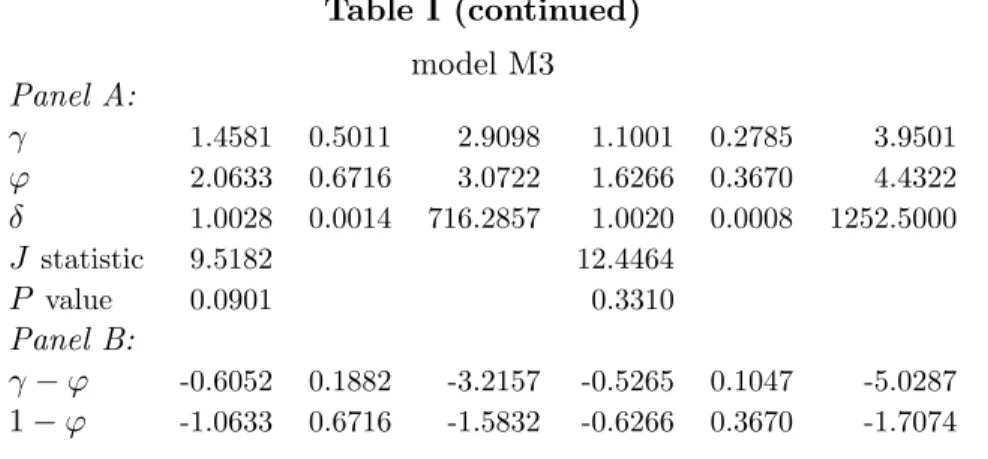
by maximum likelihood and then estimate the Euler equations (??) for the excess market return and the real risk-free interest rate with habit replaced with its estimate obtained through (??) based on the estimated values for a and λ. The estimation and test results for the Euler equations are presented under Model M2 in Table I based on the following estimated values: ba= 1.5620 andbλ= 0.7638.
When we estimate and test ARIMA models for NDS consumption, the AIC preferred model is an ARIMA(0,1,2) with a drift term, which is significantly different from zero. We therefore estimated:
△Ct+1 =a+εt+1+ (θ−(1−λ))εt−θ(1−λ)εt−1. (53)
by maximum likelihood and found ba = 1.5633 and bλ = 0.7115. The estimation and test results for the Euler equations are also given in Table I under model M3.24
The results are practically the same for both specifications. The null hypothesis H0 :
ϕ =γ is rejected at the 5% significance level for both sets of instruments. We find some evidence against the hypothesis that the absolute value of the reference level does not affect utility. For the second instrument set we can reject at the 10% level the null hypothesis
H0:ϕ= 1.25The estimate of γ−ϕis negative and significant for both sets of instruments,
which implies that durability in consumption expenditures dominates habit persistence. The value of the time preference parameter δ is greater than 1 for any set of instruments. The model is not rejected statistically at the 5% level for both sets of instruments.
Therefore, we can conclude that the data strongly reject the standard expected utility model in favor of the habit specification, that durability dominates habit persistence at
24In the next section, we conduct estimation in one stage by GMM for a more general specification which embeds the habit formation model estimated here.
the monthly level,26 and finally that there is mild evidence for both the absolute and the
relative importance of the reference level in the utility function.
3.2.3 The Reference Level as a Function of the Return on the Market Portfolio
In section 2.2.2, we have shown that given a certain specification of the reference level growth rate, we obtained generalized versions of the SDF derived by Epstein and Zin (1989) in a recursive utility framework when the certainty equivalent of future utility is of the Kreps and Porteus (1978) form. We will start by estimating the constrained version of the model described in section 2.2.3. We then estimate the generalized version of the model with the SDF in (??). The third subsection reformulates this generalized model with the habit formation model in difference as in (??), of which Campbell and Cochrane (1999) model is a particular case.
The Epstein-Zin Stochastic Discount Factor. Given that (??) is observationally
equiva-lent to the Epstein-Zin (1989, 1991) SDF when ai = 0 (i= 1, ..., n), we estimate the Euler
equations
Et
"
δ∗
Ct+1
Ct
−γ
(RM,t+1)κRf,t+1 #
= 1, (54)
Et
"
Ct+1
Ct
−γ
(RM,t+1)κ(RM,t+1−Rf,t+1) #
= 0,
jointly with the equation
△ct+1=a0+b·rM,t+1+εt+1, (55)
whereδ∗ ≡δ·exp(a0(γ−ϕ)) andκ≡b(γ−ϕ).
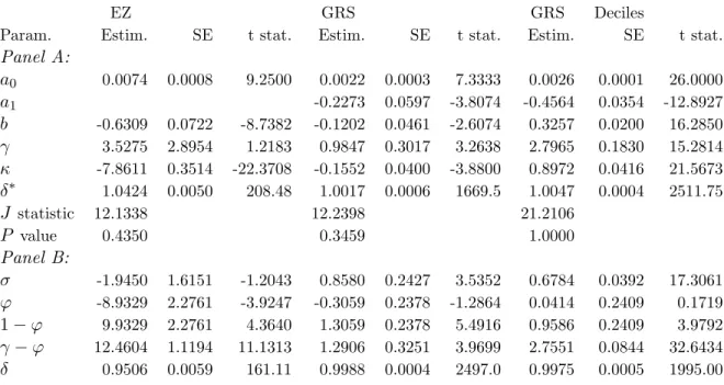
In Table II, in Column EZ, we present the estimation and test results of Euler equations (??) for the excess market return and the real risk-free interest rate together, when the latter equations are estimated jointly with the log consumption growth rate equation (??). The Euler equations are estimated with the instrument set INS2, while the instruments used to test the equation for the log consumption growth rate consists of a constant, the log real market return lagged two periods, and the log consumption growth rate lagged two periods.
The obtained point estimate of the RRA coefficient is positive (3.53) but not significantly different from zero at the 5% level. The null hypotheses H0 : ϕ= γ and H0 : ϕ = 1 are
both rejected statistically. The null hypothesis H0 :κ = 0
σ= γ1 is also rejected at the 5% significance level. The point estimate of the elasticity of intertemporal substitution is
negative (-1.95) but not significantly different from zero at the 5% level. This negative point estimate for the elasticity of intertemporal substitution is consistent with Stock and Wright (2000) who estimate the Epstein-Zin SDF (??) using US monthly data. According to Hansen’s test of overidentifying restrictions and the conventional asymptotics, the model is not rejected statistically, but again we rely on Stock and Wright (2000) to attribute this non-rejection to the poor properties of conventional asymptotics for such a specification.
A Generalized Epstein-Zin Model with Habit Formation. We now assume that the
refer-ence consumption level growth rate is a function of the previous period consumption growth rate and of the return on the market portfolio. Therefore, we estimate the Euler equations
Et
"
δ∗
Ct+1
Ct
−γ
Ct
Ct−1 κa1
b
(RM,t+1)κRf,t+1 #
= 1, (56)
Et
"
Ct+1
Ct
−γ
Ct
Ct−1 κa1
b
(RM,t+1)κ(RM,t+1−Rf,t+1) #
= 0,
jointly with the equation
△ct+1=a0+a1· △ct+b·rM,t+1+εt+1, (57)
whereδ∗ ≡δ·exp(a0(γ−ϕ)) andκ≡b(γ−ϕ).
The estimation and test results for equations (??) and (??) are presented in Table II, in Column GRS. As in the case of the Epstein-Zin pricing kernel, we use the instrument set INS2 when estimating the Euler equations and the set of instruments which consists of a constant, the log real market return lagged two periods, and the log consumption growth rate lagged two periods when estimating the equation for the log consumption growth rate. This two-period lag is important sinceεt+1 can be correlated with ∆ct.
The obtained point estimate of the RRA coefficient is in the conventional range (close to 1) and, in contrast to the case of the Epstein-Zin SDF, significantly different from 0 at the 5% significance level. The point estimate of κ is significantly different from zero and, therefore, the null hypothesis H0 :σ = 1γ is rejected at the 5% level. The estimate of the
elasticity of substitution is in the conventional range (0.85) and significantly different from 0. We reject at the 5% level the null hypotheses that the reference consumption level plays no role in asset pricing (H0 :ϕ=γ) and that an agent derives utility solely from the ratio
of his consumption to some reference level (H0 :ϕ= 1).According to Hansen’sJ statistic,
the model is not rejected statistically at the 5% significance level.27
27When the Euler equations (
As announced, we would like to test our specification under the assumption of weak identification given the poor properties of conventional asymptotics. In conducting such a test, we treat δ∗ as strongly identified andθ= (γ, σ, a0, a1, b) as weakly identified.28 Under
weak identification asymptotics, we compute a 95% confidence interval forγ in which δ∗ is concentrated out:
n
γ0 :T ScT
θ0,δb∗(θ0)
6χ2G−1,0.95 o
, (58)
whereG is the number of orthogonality conditions, ScT(θ) is the continuous updating
ob-jective function computed using a heteroscedasticity robust weighting matrix, andδb∗(θ) =
T−1PT t=1 Ct+1 Ct −γ Ct
Ct−1
(σγ−1)a1 b
(RM,t+1)(σγ −1)
Rf,t+1 !−1
.
To assess the plausibility of the GRS SDF under the weak identification assumption, we compute the S-set for γ when θ is in the conventional GMM confidence interval. The result is that our model is not rejected at the 5% significance level under weak identification asymptotics forγ >1.985, a value only slightly greater than that corresponding to the upper bound of the 5% GMM confidence set forγ. This result is consistent with that obtained by Stock and Wright (2000), who also find that the value ofγ at which the model is not rejected under the assumption of weak identification is usually higher than that under conventional normal asymptotics. However, in contrast to their result, the value of the relative risk aversion coefficient at which our model is not rejected statistically may be recognized as economically plausible.
To check whether our SDF performs better than the Epstein-Zin one in this weak identi-fication context, we compute the 95%S-set forγ for the model associated with the Epstein-Zin SDF. For the Epstein-Epstein-Zin specification of the SDF, θ= (γ, σ, a0, b) and
b
δ∗(θ) = T−1
T
X
t=1
Ct+1
Ct
−γ
(1 +RM,t+1)(σγ −1)
(1 +Rf,t+1) !−1
. (59)
We find that there is no value of γ in the 5% GMM confidence set for which the model is not rejected at the 5% significance level forθin the conventional GMM confidence set.29
The upper bound of the 5% confidence set forγ under conventional normal asymptotics is 9.20. This means that even if, as in Stock and Wright (2000), there is some value higher than this upper bound value of the risk aversion coefficient at which the model is not rejected at the 5% level, this value appears less economically plausible than for the GRS SDF..
28Givenθ,the parameterδ∗can be estimated precisely from the Euler equation for the risk-free rate of
return,δ❜∗=
✥
T−1PT t=1
✏
Ct+1
Ct
✑−γ✏ Ct Ct−1
✑(σγ−1)a1
b
(RM,t+1)(σγ−1)(1 +Rf,t+1)
✦−1
and, hence, is strongly
identified by a constant.