The Capm and Fama-French models in Brazil: a comparative study

(1)

Fundação Getulio Vargas

Escola de Economia de São Paulo

The CAPM and Fama-French Models in Brazil: A

Comparative Study

Fernando Daniel Chague

(2)

Fernando Daniel Chague

The CAPM and Fama-French Models in Brazil: A

Comparative Study

Dissertation presented to the Escola de

Economia de São Paulo, Fundação Getulio

Vargas as one of the requirements for

completion of the Masters in Economics

Advisor: Rodrigo De Losso da Silveira Bueno.

(3)

The CAPM and Fama-French Models: A

Comparative Study

Fernando Daniel Chague

1

Escola de Economia de São Paulo

Fundação Getulio Vargas

November 22, 2007

(4)

Abstract

This paper confronts the Capital Asset Pricing Model - CAPM - and the 3-Factor Fama-French - FF - model using both Brazilian and US stock market data for the same sample period (1999-2007). The US data will serve only as a benchmark for comparative purposes. We use two competing econometric methods, the Gener-alized Method of Moments (GMM) by Hansen (1982) and the Iterative Nonlinear Seemingly Unrelated Regression Estimation (ITNLSUR) by Burmeister and McElroy (1988). Both methods nest other options based on the procedure by Fama-MacBeth (1973). The estimations show that the FF modelfits the Brazilian data better than CAPM, however it is imprecise compared with the US analog. We argue that this is a consequence of an absence of clear-cut anomalies in Brazilian data, specially those related to firm size. The tests on the efficiency of the models - nullity of intercepts and fitting of the cross-sectional regressions - presented mixed conclusions. The tests on intercept failed to rejected the CAPM when Brazilian value-premium-wise portfolios were used, contrasting with US data, a very well documented conclusion. The ITNLSUR has estimated an economically reasonable and statistically significant market risk premium for Brazil around 6.5% per year without resorting to any par-ticular data set aggregation. However, we could not find the same for the US data during identical period or even using a larger data set.

Keywords: CAPM, Fama-French, ITNLSUR, GMM, risk-premium.

(5)

Este estudo procura contribuir com a literatura empírica brasileira de modelos de apreçamento de ativos. Dois dos principais modelos de apreçamento são confronta-dos, os modelos Capital Asset Pricing Model (CAPM) e de 3 fatores de Fama-French. São aplicadas ferramentas econométricas pouco exploradas na literatura na-cional na estimação de equações de apreçamento: os métodos de GMM e ITNLSUR. Comparam-se as estimativas com as obtidas de dados americanos para o mesmo período e conclui-se que no Brasil o sucesso do modelo de Fama e French é limi-tado. Como subproduto da análise, (i) testa-se a presença das chamadas anomalias nos retornos, e (ii) calcula-se o prêmio de risco implícito nos retornos das ações. Os dados revelam a presença de um prêmio de valor, porém não de um prêmio de tamanho. Utilizando o método de ITNLSUR, o prêmio de risco de mercado é positivo

e signiﬁcativo, ao redor de 6,5% ano.

Palavras-Chaves: CAPM, Fama-French, ITNLSUR, GMM, prêmio de risco.

(6)

1 Introduction

This paper confronts the Capital Asset Pricing Model - CAPM - and the 3-Factor Fama-French - FF - model using both Brazilian and US stock market data for the same sample period (1999-2006). The focus is on the Brazilian data analysis, since the results for the US are widely known. Therefore, the US data will serve only as a benchmark for comparative purposes. We use two competing econometric methods, the Generalized Method of Moments (GMM) by Hansen (1982) and the Iterative Nonlinear Seemingly Unrelated Regression Estimation (ITNLSUR) by Burmeister and McElroy (1988). Both methods nest other options like the Generalized Least Squares (GLS), the Ordinary Least Squares (OLS) and the Weighted Least Squares (WLS) frameworks based on the procedure by Fama-MacBeth (1973). Although GMM method accounts for possible autocorrelated errors, it has a poor performance on small samples. The ITNLSUR is strongly consistent and asymptotically normally distributed hence it is robust with respect to non-normal errors. However, while it assumes heteroskedasticity errors, it does not takes into account possible error autocorrelations.

The estimations show that the FF model fits the Brazilian data better than CAPM, however it is imprecise compared with the US analog. We argue that this is a consequence of an absence of clear-cut anomalies in Brazilian data, specially those related to firm size. The tests on the efficiency of the models - nullity of intercepts and fitting of the cross-sectional regressions - presented mixed conclusions. The tests on intercept failed to rejected the CAPM when Brazilian value-premium-wise portfolios were used, contrasting with US data, a very well documented conclusion. The ITNLSUR has estimated an economically reasonable and statistically significant market risk premium for Brazil around 6.5% per year without resorting to any par-ticular data set aggregation. However, we could not find the same for the US data during identical period or even using a larger data set.

The CAPM model of Sharpe (1964) and Lintner (1965) embodies the agents’ behavior features of Markowitz (1952), and establishes a theoretical relationship be-tween asset returns that can be tested empirically. The empirical evidence, however, has pointed against the theory since its very beginning. Black, Jensen and Scholes (1972) and Blume and Friend (1975) found out a constant diﬀerent from the risk free asset return in the post-war period. Fama and MacBeth (1973) achieved the same conclusion, although theβ factor presented some predicted characteristics.

(8)

captured by the βs. For instance, portfolios containing firms with low market value or low book value to market value ratio turned out to have higher returns than CAPM predicted. Moreover the literature documented other "anomalies" due to portfolios grouped according to earnings-price ratio, momentum and calendar effect (January and Fridays have returns significantly different from other months or days).

In view of such an empirical evidence, Fama and French (1992, 1993) propose a multifactorial model capable of explaining such anomalies In addition to the CAPM’s factor, two other explanatory variables are added: a premium for the ﬁrm size and a premium for the market value relative to the book value. The inclusion of those factors improved sensibly the model ﬁtting to the US empirical data.

CAPM and FF models deliver some testable predictions. In this paper we will focus on the following: null hypothesis that the intecepts of the time series regressions are zero; the cross section return adjustments betweenfitted and actual data; whether the risk premium coefficient of the market portfolio is positive; whether the risk premium coefficients are equal to the time means of the factors returns.

To perfom the tests, the market portfolio used will be the Bovespa stock mar-ket index - Ibovespa - which groups together the more liquid stocks in Brazil. For robustness, we also consider other benchmarks for the market portofolio. The first is the portofolio based on the Morgan Stantely Capital Internation methodology -MSCI. The second portfolio is the aggregation, equally weighted, of all the stocks in our database. Finally, the last portfolio weights the stocks based on their market value. In addition, the models will be tested on three different set of assets. Two are portfolios sets, each with 10 portfolios grouped according to thefinancial charac-teristics: market value (ME) and the ratio book value over market value (BE/ME). The third set consists of the 44 out of 60 more representative stocks in the Ibovespa, without any aggregation of returns.The motivation for using portfolios grouped as mentioned follows the literature on anomalies (see Fama and French, 1996), which inspired the FF model1_{. The third set of assets o}_ff_{ers an additional test, specially}

regarding the FF model, which was taylored to explain such anomalies.

Gibbons, Ross and Shanken (1989) and MacKinlay and Richardson (1991) suggest procedures for testing whether the intercepts of the portfolios are jointly null. As will be seen, the results for the Brazilian data are contradictory, depending on the proxy for the market portfolio and on the portfolios used as assets. However, it predominates the non rejection of the null, which is consistent with theory. The

1_{Studies have usually focused on the 25 portfolios used by Fama and French (1993). Each of}

(9)

estimates are important because both methodologies are applied with distinct market portfolios, which increases the support for eventually more solid remarks, specially when compared to Málaga and Securato (2004), for instance. By contrast, the US data produced important diﬀerences between the CAPM and FF models. The FF model reduced vigorously the CAPM pricing error, mainly when the entire sample, 1963:07 to 2006:08, is used.

The estimations for Brazil using portfolios aggregations revealed a strong value premium (market value/book value), but none size premium. Reﬂecting thisﬁnding, the FF model adjusts better than the CAPM where anomalies are relevant in terms of mean absolute princing error.

From the cross section returns, we show that the Brazilian risk premium is sta-tistically positive and around 6.5% per year using the ITNLSUR estimation method. The data used to estimate the risk premium consists of the 44 more liquid stocks composing the Ibovespa stock market index. This result is particularly important because it avoids using foreign data and arbitrary assumptions to calculate the cost of capital of firms, given the widespread market practice of using the CAPM to evaluate afirm’s cashflow.2

The work is divided in the following way. In the next section, we present the portfolio composition and data to be used in this work. In the section 3, we present the theory and econometric tests that are executed in the section 4. Also this last section develops the analysis of the results. Finally the last section concludes.

2 Data Set and Portfolios Construction

2.1 Data Set

This study uses a data set containing 172 stock prices of 123 ﬁrms, all of them traded in the São Paulo Stock Exchange - Bovespa. To avoid eventual distortions related to the change in the Brazilian exchange rate regime, the sample used spans from January 1999 to August 2006.

Financial data were obtained from both Economática data set and Bovespa web-site for completion and double checking3_{. All prices are closing prices, adjusted for}

splits and dividends, and were included according to the following criteria:

2_{In Brazil, there is an argument over the empirical content of CAPM. Some studies document}

anomalies and look for multifactorial models (see, for instance Costa, Leal and Lemgruber, 2000).

3_{Firms must send}_ﬁ_{les as Standard Financial Balance Sheet (DFP) and Quarterly Information}

(10)

1. Missing data for 3 or more consecutive months were excluded from the sample4_;

2. Missing data wasﬁlled by linear interpolation between the last and the follow-ing observed price5_.

The return of asseti= 1,2, . . . , N at timet= 1,2, . . . , T is deﬁned as:

Ri,t = ln

µ

Pi,t

Pi,t−1

¶

,

wherePit is the price of asset i at timet.

The market portfolio follows the convention of other researchers of taking the Ibovespa index. That index is composed with the more liquid stocks of Bovespa. However, for robustness purposes, other proxies for the market portfolio are also used and the results are reported in the appendix.

As usual in Brazil, the risk free rate was calculated from the Selic interest rate. Since it is given yearly, the risk free rate at montht,Rf t is:

Rf,t=

ln (1 +Selict)

12 .

US results are used as benchmark and comparative purposes. The porfolios for Americanﬁrms are from CRSP website and Kenneth French’s website6_{. The sample}

period starts in July 1963 and ends in August 2006. There are stocks traded in NYSE, AMEX and Nasdaq (together, they counted for more than 4,000 ﬁrms in 2006).

2.2 Portfolio Construction

This work aims at testing asset pricing models with Brazilian data under several speciﬁcations, as we consider three data sets. Theﬁrst set consists of the more liquid stocks in Bovespa and, consequently, represents most of the volume traded in the exchange house. Indeed, out of 57 stocks composing Ibovespa in the last quarter of

4_{There are two exceptions, though. The stocks PRGA4 and CMET4 left Bovespa oﬀ}_{during the}

last 4 and 3 months before the sample end up, respectively. In that case, we kept the last price traded during such months.

5_{BRKM3 and PEFX5 were the only two stocks with more than 10% of months interpolated.}

Besides these two, other 42 stocks had at least one month interpolated. Of these, on average 2.9 non consecutives months were interpolated.

(11)

2005, the criteria deﬁned in the last section leave us with 44 stocks for 92 months. In this set, the stocks are not aggregated in any way at all, and it will serve as a "control" group allowing us to compare results with those of composed portfolios in ways to be described soon. Note that a desirable property of the asset pricing model is that it can explain return diﬀerences regardless how assets are grouped.

The other two data sets follow studies that pointed out returns not explained by the theory, the so-called anomalies. We focused on the ﬁnancial indexes that presented the most challenge to the CAPM model: size and ratio between book equity and size. Size is measured by the market equity value - ME - that is, the number of stocks, ordinary and preferred, times the market price7_{. The ratio book}

equity and size - BE/ME - is measured by the ratio of total assets minus total liabilitites and size (as deﬁned above).

The 123 ﬁrms were ranked yearly in 10 groups, either by ME or BE/ME, ac-cording to the balance sheet of December of each year. The return of each portfolio is the arithmetic mean of the stocks’ returns, hence it is equally-weighted as are the portfolios from US data. Appendix provides more details about the portfolios’ composition8_.

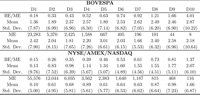
Table I shows the statistics from the two sets of portfolios compared with simi-larly composed US portfolios during the same period. The portfolios are ranked in ascending order in terms of expected return, "anomaly-wise". That is, portfolio 1 containsﬁrms with the lowest BE/ME and the highest ME, inversely to portfolio 10.

Table I

Descriptive Statistics BE/ME and ME. Data from Bovespa, NYSE, AMEX and Nasdaq

Monthly returns in local currency, between January 1999 and August 2006. The porfolios are based on December 2005. ME corresponds to the average size of theﬁrms in US$ million. All portfolios are equally-weighted. Dx represents the x-th decile.

7_{Preferred stock in Brazil is not the same as in the US. It means that the owner are not allowed}

to vote and that dividends must go to owners of preferred stock atﬁrst.

(12)

BOVESPA

D1 D2 D3 D4 D5 D6 D7 D8 D9 D10

BE/ME 0.18 0.33 0.43 0.52 0.63 0.74 0.92 1.21 1.66 4.01

Mean 1.36 1.89 2.37 2.57 1.80 2.53 2.62 2.49 2.46 2.87

Std. Dev. (7.87) (6.99) (6.96) (6.50) (7.14) (6.82) (7.05) (6.20) (6.90) (10.22)

ME 23,283 5,370 2,425 1,588 667 405 196 101 44 8

Mean 2.42 2.04 1.81 2.20 3.01 2.03 1.66 2.40 2.58 2.18

Std. Dev. (7.90) (8.15) (7.65) (7.26) (6.61) (6.15) (5.53) (6.32) (6.96) (10.64) NYSE/AMEX/NASDAQ

BE/ME 0.15 0.26 0.35 0.39 0.46 0.53 0.61 0.73 0.81 1.37

Mean 0.13 0.83 0.98 1.14 1.34 1.60 1.55 1.55 1.77 2.07

Std. Dev. (9.76) (7.52) (6.39) (5.67) (5.07) (4.89) (4.56) (4.51) (5.11) (6.10) ME 55,576 12,044 6,035 3,562 2,383 1,640 1,187 815 468 116

Mean 0.10 0.61 0.68 0.89 0.61 0.64 0.63 0.87 0.98 1.66

Std. Dev. (5.00) (4.95) (5.81) (5.61) (5.77) (6.53) (6.62) (6.64) (7.23) (6.87)

It is vastly documented in the economic literature the existence of a return dif-ferential between the extreme portfolios classified by ME and BE/ME. For the US, such a differential is1.94% per month (D10₋D1) in portfolios ordered by BE/ME (1.44% per month if one takes quintiles9_{). Similarly, the di}_ff_{erential in portfolios}

ordered by ME is positive, about1.56% per month (0.97% in quintiles).

Brazilian data follows similar pattern when the portfolios are ordered by BE/ME, but not when they are ordered by ME. In thefirst case, the difference is1.51% per month (1.04% in quintiles). In the second case, the difference is practically nill:

−0.24% (0.15% in quintiles).

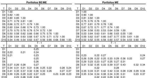
Another feature identified in US data is a high degree of autocorrelation, which is important to the choice of econometric methods to be used to estimate the model pa-rameters. Table II presents the autocorrelation coeficients and the cross-correlation when the statistics overcomes two standard-deviations (±2/√T) between the series. The series are well correlated in general with coefficients higher than0.50. All series are cross-correlated, and one-lagged correlations are significant to roughly half of the series. Other lags are not significant at all.

Table II

Serial Correlation Between Portfolios BE/ME and ME (BOVESPA)

Cross-correlation between monthly returns (panel T; symmetric matrix) and lagged 1 month (panel T-1). Standard-deviation higher than(2/√T).

(13)

T D1 D2 D3 D4 D5 D6 D7 D8 D9 D10 T D1 D2 D3 D4 D5 D6 D7 D8 D9 D10

D1 1.00 D1 1.00

D2 0.82 1.00 D2 0.90 1.00 D3 0.80 0.85 1.00 D3 0.81 0.82 1.00 D4 0.71 0.79 0.81 1.00 D4 0.75 0.76 0.76 1.00 D5 0.66 0.72 0.71 0.79 1.00 D5 0.77 0.81 0.79 0.78 1.00 D6 0.60 0.64 0.68 0.74 0.73 1.00 D6 0.67 0.72 0.71 0.77 0.74 1.00 D7 0.70 0.70 0.76 0.78 0.74 0.72 1.00 D7 0.54 0.58 0.53 0.53 0.64 0.59 1.00 D8 0.50 0.58 0.62 0.66 0.66 0.75 0.76 1.00 D8 0.53 0.64 0.63 0.61 0.66 0.63 0.55 1.00 D9 0.58 0.64 0.63 0.68 0.67 0.70 0.71 0.72 1.00 D9 0.59 0.62 0.67 0.66 0.67 0.77 0.55 0.61 1.00 D10 0.54 0.49 0.54 0.62 0.67 0.56 0.66 0.68 0.66 1.00 D10 0.52 0.52 0.55 0.58 0.60 0.57 0.54 0.53 0.60 1.00

T D1 D2 D3 D4 D5 D6 D7 D8 D9 D10 T D1 D2 D3 D4 D5 D6 D7 D8 D9 D10

D1 0.25 D1

D2 0.22 0.21 0.24 D2

D3 0.21 0.23 D3 0.23 0.22 0.27 0.24 D4 0.25 D4 0.26 0.28 0.22 0.25 0.33 0.29 0.36 0.22 0.27 D5 0.26 D5 0.29 0.23 0.23 0.27 0.25 0.27 0.31

D6 0.27 0.26 0.28 0.27 D6 0.31 0.32 0.35 0.33 0.39 0.37 0.43 0.32 0.34 D7 0.34 0.31 0.31 0.31 0.36 0.25 0.22 0.28 0.24 D7 0.22 0.28

D8 0.41 0.35 0.37 0.32 0.36 0.33 0.26 0.27 0.27 D8 0.35 0.33 0.31 0.42 0.42 0.34 0.28 0.28 0.29 0.34 D9 0.30 0.26 0.28 0.22 0.27 0.25 0.23 0.28 0.23 D9 0.35 0.34 0.34 0.38 0.34 0.35 0.31 0.23 0.37 D10 0.23 0.26 0.22 0.26 D10 0.22 0.22 0.29 0.30 0.31

Portfolios BE/ME

T

T - 1

Portfolios ME

T

T - 1

2.3 Market Portfolio and Factors

The Bovespa Index (IBOV) is the main proxy for market portfolio in Brazil. In order to make this paper comparable to others, we take IBOV as our proxy, but leave in the appendix the results with other proxies like the Morgan Stanley Capital International for Brazil (MSCI-Brazil) and two other alternative proxies. The ﬁrst is made up of all stocks in our database equally weighted (BEW). The second all stocks are weighted by the market value of the ﬁrms (BVW). Next table presents the basic statistics of these indexes in terms of returns.

Table III

Descriptive Statistics: Market Portfolios and Risk Free Rate

Percentual mean and standard-deviation. Correlation between January 1999 and August 2006 (92 months).

Correlation

Mean Std-dev t(mean) Sharpe IBOV MSCI BVW BEW

SELIC 1.48 0.32 43.8

IBOV 1.82 8.64 2.02 0.041 1

MSCI 1.92 7.54 2.45 0.059 0.937 1

BVW 3.03 7.25 4.01 0.214 0.958 0.966 1

(14)

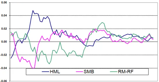
Because the CAPM is not able to explain premia and returns of portfolios based on ME and BE/ME, Fama and French (1992) suggest instead a multifactorial model. Accordingly, they add two other factors to the CAPM, named SMB and HML (SMB

-small minus big and HML - high minus low). SMB corresponds to the diﬀerential

returns betweenﬁrms of big size and small size. HML corresponds to the diﬀerential returns between portfolios with high and low BE/ME. We, then, construct such indexes for Brazil following these authors (see appendix for details on the construction of these indexes).

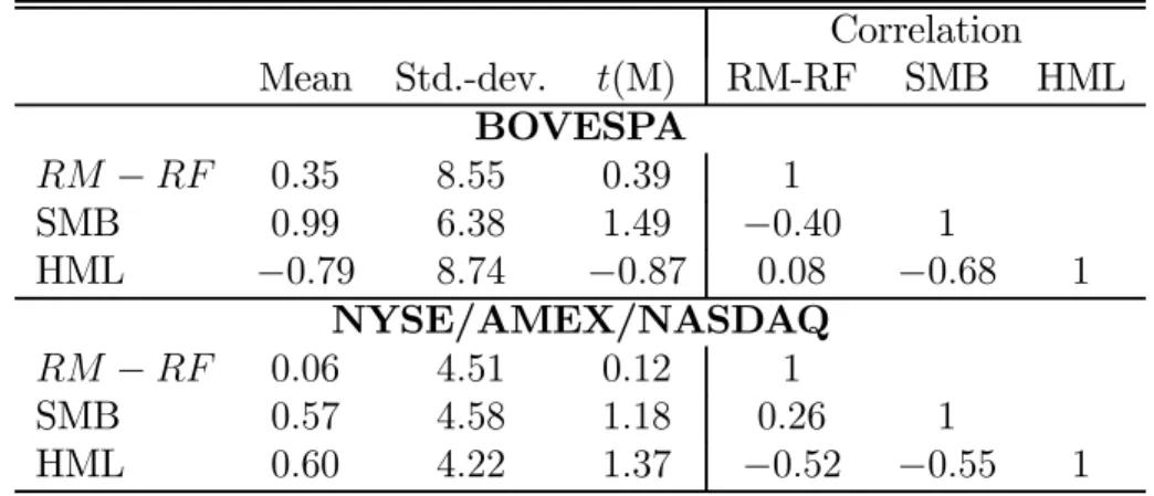
It is desirable that the factors are not correlated. For example, Fama and French (1995) point that between July 1963 and December 1992, the correlation between them is−0.08. Notwithstanding, possibly because of the short period of time avail-able, the Brazilian series HML and SMB are highly correlated. Table IV shows a correlation between such series around −0.68. However, for the same 92 months, Fama and French’s data have a correlation of −0.55. In addition, the unconditional mean of all factors are not statistically signiﬁcant both for Brazilian and US data.

Tabela IV

Descriptive Statistics - 3 Factors - BOVESPA, NYSE,AMEX and Nasdaq

Percentual mean and standard-deviation. Correlation between January 1999 and August 2006 (92 months). In panel Bovespa, the factor RM-RF is the monthly excess return between Ibovespa and Selic. In panel NYSE/AMEX/Nasdaq, RM-RF is the excess return between the value-weighted portfolio and the US T-Bill of one month.

Correlation

Mean Std.-dev. t(M) RM-RF SMB HML

BOVESPA

RM₋RF 0.35 8.55 0.39 1

SMB 0.99 6.38 1.49 −0.40 1

HML ₋0.79 8.74 ₋0.87 0.08 ₋0.68 1

NYSE/AMEX/NASDAQ

RM₋RF 0.06 4.51 0.12 1

SMB 0.57 4.58 1.18 0.26 1

HML 0.60 4.22 1.37 −0.52 −0.55 1

3 Theory and Econometric Tests

(15)

E[Ri,t−Rf,t] =λmβi (1)

for everyt= 1,2, . . . , T, where

λm is the risk price or risk premium given byE[Rm,t−Rf,t] ;

Rm,t is the return of the market portfolio at time t; and

β_i is the amount of risk in portfolioi.

The coeﬃcient βi may be estimated by ordinary least squares according to the

following equation:

Ri,t−Rf,t =αi+βi(Rm,t−Rf,t) +εi,t (2)

for everyi= 1,2, . . . , N.

The CAPM theory generates three main implications that may be tested (Camp-bell, Lo and MacKinlay (1997)):

1. The intercept is zero in equation (2);

2. The risk premium is positive λm >0;

3. There is a linear relationship betweenβs and expected return, following equa-tion (1).

As a matter of fact, the empirical evidence regarding the US usually rejects the theory. Blume and Friend (1975) and Black, Jensen and Scholes (1972) report an intercept diﬀerent from zero, specially in the post-War period. Fama and MacBeth (1973)10 _con_ﬁ_{rmed their results, although they have not rejected the other two}

im-plications of equation (1).

In order to take into account some of these stylized facts, Black (1972) relaxes the assumption about the existence of a risk free asset and introduces the zero-beta portfolio, which is a minimum variance portfolio uncorrelated with the market port-folio. On the other hand, Roll (1977) criticizes the proxy for the market portfolio by arguing that it contains only observed asset returns, rather than representing the re-turns of the entire economy. The market portfolio, hence, would not be observable,

10_{In that work, the authors introduce as estimation methodoloy known as 2-stage Fama and}

MacBeth methodoloy. The portfolios are ordered according to theβsmagnitude, in order to reduce dispersion, which would make insigniﬁcant parameter λm. Thus, in the ﬁrst stage, one estimates

by OLS eachβ using time series data. In the second stage, the estimatedβsbecome explanatory variables of the mean returns of the portfolios at each time t. The total risk premium is then obtained by averaging the risk premia of each time OLS estimation of λm, and the

(16)

because any possible proxy one can think of cannot consider intangible assets for example, therefore the theory is not testable. In view of this situation, Ross (1976) proposes another model, named arbitrage pricing theory (APT), with assumptions less restrictive than the CAPM11_{. In fact, by resuming portfolio choices to choices}

over mean-and-variances, the CAPM implicitly assumes a direct relationship between wealth and consumption, which is a very restrictive hypothesis considering there is a temporal dynamics between these variables. As a consequence, Merton (1973) intro-duces an intertemporal asset pricing model, heavily criticizing the static assumption of the CAPM. The models of Lucas (1978) and Breeden (1979) follow that line of representative agents and formulate the consumption CAPM theory, also known as CCAPM. In those models, the decisions about where allocating wealth result from an intertemporal maximization of the utility function, where the consumption is the controlled variable and theﬁnancial markets enters in order to smooth consumption over time.

Parallel to the theoretical development described, new empirical evidence came out, heavily questioning the CAPM. In particular, assets grouped together according the ﬁnancial characteristics of ﬁrms as size, book value and dividends presented returns unexplained by β (BASU (1977), Banz (1981) and Rosenberg, Reid and Lanstein (1985)).

Such an evidence has motivated Fama and French (1992, 1993) to estimate a multifactorial model by including somead hocfactors taylored to capturate observed anomalies. Thus the expected excess return between the portfolio (Ri) and the risk

free rate (Rf) responds to three factors: the excess return of the market portfolio,

the return spread between portfolios with big and smallﬁrms,SMB, and the return spread betweenﬁrms with high and low BE/ME, HML:

E[Ri,t−Rf,t] =λmβi+λssi+λhhi (3)

whereλi,i=m, s, h, are the expected premia, respectively measured byE[Rm−Rf],

E[SMB]andE[HML]. The coeﬃcients(β_i, si, hi) measure the portfolioi

sensitiv-ity to each factor and are obtained through the time series regression:

Ri,t−R,f,t =ai+βi(Rm,t−Rf,t) +siSMBt+hiHMLt+εt,i (4)

In equilibrium, agents require that premium to oﬀset the risk of owning such assets. Fama e French do not provide a theory based of primitive foundations to

11_{For instance, the CAPM demands homogeneous agents with quadratic preferences or}

(17)

justify why using exactly those factors. However, Fama e French (1996) argue that

firms with profits sistematically low are facingfinancial difficulties and tend to have a high BE/ME. Given that additional risks, returns must be higher in equilibrium. By contrast, consolidadedfirms have low BE/ME, hence a low return, independently of other risks. Similarly, the market value of afirm may on average indicates a negative

financial status or reflects a natural risk of an incipient firm. In such case, returns ex-ante must reflect such additional risks.

This paper tests the implication of the CAPM and the three factors model of Fama and French, FF, for Brazil and the US. The tests focus on two basic implications of the models:

1. The intercepts are jointly null for all assets in the time series regressions rep-resented by equations 2 and 4;

2. The cross-section adjustment between the expected return predicted by the model and the observed mean return, according to equations 1 e 3.

A by-product of the procedure is to estimate the risk premium for Brazil, spreadly used by market practitioners for evaluating cashﬂows of corporations. However, we do not test formally another possible implication regarding whether the risk premium is the expected excess return, λm =E(Rm,t−Rf).

3.1 Test of Intercepts

By assumption, the multifactorial model is able to capturate the behavior of returns. Such an implication will be true if the intercepts are all null. A usual test for that implication is suggested by Gibbons, Ross and Shanken (1989). However, the test does not adjust for autocorrelated series, which is a feature often found in ﬁnancial series. Alternatively, one may use the test by MacKinlay e Richardson (1991), based on the overidentiﬁcation test using GMM estimation method.

In this work, we perform and compare both alternatives. Therefore, let us de-scribe each one in what follows.

3.1.1 Gibbons, Ross e Shanken’s (1989) Test

Using the OLS estimates of equation 4, one can test the null hypothesis that

αi = 0 ∀ i. If the disturbances are temporally independent and jointly normal, with

(18)

GRS =

µ

T N

¶ µ

T ₋N ₋K T −K−1

¶ "

ˆ

a0ˆ

Σ−1_ˆ_a

1 + ˆμ0

fΣˆ−f1μˆf

#

∼F(N, T ₋N ₋K) (5)

where ˆ

a is anN ×1 vector of constants estimated by either equation 2 or 4; ˆ

Σ is an N ×N residual covariance matrix; ˆ

μ_f is aK×1 factors means12_{; and}

ˆ

Σf is aK×K factor covariance matrix.

3.1.2 Overidentiﬁcation Test

An advantage of the GMM estimation over the OLS model (used in the GRS test) is that GMM does not assume any hypothesis over the distribution of the series like

i.i.d.(serial uncorrelatedness and homoskedasticity). However, in general, financial series do present at least autocorrelation. Therefore, MacKinlay and Richardson (1991) suggest two tests through GMM to overcome the difficulties of the GRS test. Thefirst test consists of estimating(α,β0

)0 by GMM and testing the null hypothesis that αi = 0, ∀ i, where β

0

is the vector of factor coeﬃcients.

The second test consists of imposing αi = 0,∀i, estimating the model by GMM,

and then testing whether the objective function at the minimum is statistically null. That is, use a vector of ones as instrument, and, if the null is false, the objective function will fail in being statistically zero. We perform this second test in this work. Therefore, letri,t =Ri,t−Rf,t, and deﬁne the population moments in the following

way:

E[g(w_t_,_β

0)] = E

∙ _r

t−β

0 0ft

(r_t₋_β0

0ft)⊗ft

¸ = ∙ ₀ 0 ¸ (6) where

r_t _{= [}_r₁_,t_{, r}₂_,t_{. . . , r}_N,t_]0 _{is an} _N _×₁ _{vector of excess returns;} f_t _{is a} _K_×₁_{vector of factors;}

⊗ is the Kronecker operator.

By assumption data is ergodic, therefore the population moments have a sample analog given by:

gT (w,β) =T−1 T

X

t=1

g(w_t_,_β)_,

(19)

wherew_t _{is a vector of observed variables.} The GMM estimator gives us βˆgmm = arg

β

min{QT (β)}, from:

QT (β) =gT (w,β)

0

W_T_g_T ₍w_,_β)_, ₍₇₎

whereW_T _{is a matrix that weights e}ﬃ_{ciently each moment.}

There are more moments than parameters to be estimated. It is necessary to estimate NK coeﬃcients (N portfolios and K parameters in each), and there are

N(K + 1) moment conditions, every portfolio is multiplied by the factor plus the conditions that the errors are zero in each portfolio. Hence, the model is overidentiﬁed and, as such, the quantity QT

³

ˆ

βgmm´ follows a χ2 _{distribution with} _N _{degrees of}

freedom (Hansen (1982)). Consequently, it can be statistically tested. If we fail to reject the null that all moments are statistically zero, them the model is correctly identiﬁed and, consequently the intercepts are statistically jointly null.

3.2 Risk Premium

The popularity of the CAPM and FF models probably resides in the fact that they establish a straightforward relationship of return differentials through the pricing equations (1) and (3). A natural way of testing the models emerges, the coefficients significance and sign of the cross-sectional pricing equation, between excess returns andβ_s.

However, since the βs are estimated in the ﬁrst step, it is needed to adjust the variance of the estimated parametersλsin the second step. This motivated Fama and MacBeth (1973) to propose the OLS estimation in two stages. However, nowadays there are other techniques which make Fama and MacBeth’s procedure obsolete. They are the GMM and the ITNLSUR.

Importantly, Shanken and Zhou (2007) recently have studied the small sample properties of cross-sectional expected return estimators like GMM, Maximum Like-lihood, Fama and MacBeth’s (1973) procedure and some variants as the Generalizes Least Squeares - GLS - and the Weighted Least Squares - WLS . They conclude that all estimators are identical for samples greater than960observations (30years). GMM performs as well as the other methods for N = 48 and T > 120. However, GMM gets worse whenN = 25.

(20)

3.2.1 ITNLSUR

Burmeister and McElroy (1988) proposed a new econometric model to estimate the cross-sectional expected returns. Their model focuses on the APT, but it can be used for testing the CAPM and the FF models. The method is an iterated nonlinear seemingly unrelated regression and meant to correct many problems related with the two stage methods (OLS, GLS, WLS). Among the deﬃciencies associated with the conventional methods are the unrobustness of the estimates under non normality, loss of estimation eﬃciency, non uniqueness of the second stage estimators due to the need of grouping assets in portfolios and problems with statistical inference.

This section presents brieﬂy the model by Burmeister and McElroy (1988), in order to make it clear how it works. Thus, consider a multifactorial model with K

factors andN assets. The ITNLSUR methods allows one to estimate simultaneously theNK βs and theK λs, through the econometric model:

Ri,t −λ0,t = K

X

j=1

β_ij(λj +fj,t) +εi,t, (8)

where, in principle, λ0,t is observed and will stand for the risk free asset.

Notice in the model that β_ij multiples both fj,t (conventional ﬁrst stage) and

λj (conventional second stage) simultaneously. That’s the way that Burmeister and

McElroy (1988) nest all model into one. Also, it is assumed that

Et[εi,t] = 0;

Et[εi,tεj,s] =

½

σij, t=s

0, t6=s ; and Et[εi,t|fj,s] = 0.

Observe that there is no assumption about the error distribution. And when the errors are multivariate normal, then the estimator is a maximum likelihood estimator. Let ρ_i ≡ Ri,t−λ0,t be a T ×1 vector representing the temporal excess returns

and rewrite the model in the following way (8):

ρ_i = [λ0

⊗1_T ₊f_]_β

i+εi =X(λ)βi+εi fori= 1, ..., N,

where

λ is aK ×1vector of risk premia, depending on the factor loading;

(21)

1_T _{is a}_T _×₁_{vector of ones; and} X_(λ) _{is a}_T _×_K _matrix.

Stacking the N equalities above, one gets:

ρ≡ ⎛ ⎜ ⎝ ρ₁ ... ρ_N ⎞ ⎟ ⎠= ⎡ ⎢ ⎣

X_(λ) 0 _{· · ·} 0 ... ... ... ... 0 0 _{· · ·} X_(λ)

⎤ ⎥ ⎦ ⎛ ⎜ ⎝ β₁ ... β_N ⎞ ⎟ ⎠+ ⎛ ⎜ ⎝ ε1 ... εN ⎞ ⎟ ⎠.

Rewriting more compactly, one gets:

ρ= [IN ⊗X(λ)]β+ε, (9)

where β= [β0

1, β 0

2, . . . , β 0

N]

0

; ε= [ε0

1, ε 0

2, . . . , ε 0

N]

0

;

The estimation process involves several steps. Firstly, the parameterˆθ =³ˆaij,βˆij

´

,

where ˆaij = βijλ, is obtained by OLS conventionally, following equation (8). Then

the residuals are used to estimate the covariance matrix given by Σˆ = [T−1_ˆ_e0

iˆej].

Then, the parameters ³β,˜ λ´ are obtained iteratively, by minimizing the quadratic error of equation (9):

Q³λ,β; ˆΣ´= [ρ₋[IN ⊗X(λ)]β]

0³_ˆ

Σ−1 _⊗IN

´

[ρ₋[IN ⊗X(λ)]β].

The process follows iteratively until covergence, using the estimated values³β˜s,λs´ to generate Σˆs _{and to minimize} _Q³_λ_{, β}_{; ˆ}_Σs´_{. Notice that the process is not more}

than quadratic residuals minimizations, which implies estimators strongly consistent and asymptotically normal, even when the errors are not normally distributed.

3.2.2 GMM

(22)

However, GMM has not been much used to estimate the cross-section returns in equation (1). According to Shanken and Zhou (2007), the reason for that is the difficulty in finding out numerical solutions for the problem, since there are a large number of parameters to estimate coupled with the nonlinearity of the model. Therefore, if the problem can be linearized in some way and conveniently weighted, then those difficulties may be overcome.

In line with this argument and following Harvey and Kirby (1995), Shanken and Zhou (2007) suggest estimating the model sequentially. To see how it works, deﬁne R_t _{as the}_N _×₁ _{vector of portfolios or assets to which corresponds an}_N _×₁_vector of means,μ_r, that is:

E(R_t_{) =}_μ_r_.

Similarly, let f _{be a} _K _×₁ _{vector of factor to which correspond another} _K _×₁ vector of factor means,μ_f:

E(f_t_{) =}_μ_f_.

LetΣf be a K×K factor covariance matrix, such that:

Eh¡f_t₋_μ

f

¢ ¡_f

t−μf

¢0i

=Σf.

The matrix contains K(K₂+1) distinct covariances. To obtain a vector of these covariances, apply the VECH operator, which stacks the columns of the lower portion of a covariance matrix, such that:

E³vechh¡f_t₋_μ

f

¢ ¡

f_t₋_μ

f

¢0i´

=vech(Σf).

Finally, the last N moment conditions requires that the cross-sectional error are jointly zero. Thus, let the covariante between returns and factor be aN×K matrix, Σrf, such that:

E¡R_t₋_γ

01N −ΣrfΣ−f1γk

¢

=0_,

where γk is a K×1 vector of parameters. If K = 1, then this could be the market

premium, for example.

Putting together all the moment conditions, one obtains:

E[g(w_t_,_θ₀_{)] =} _E ∙

g1¡wt,θ10

¢

g2¡wt,θ10,θ20

¢ ¸ = = E ⎡ ⎢ ⎢ ⎢ ⎣

R_t₋_μ

r

f_t₋_μ

fk

vechh¡f_t₋_μ

f

¢ ¡_f

t−μf

¢0

−Σf

i

R_t₋_γ

01N −ΣrfΣ−_f1γk

(23)

Notice the N ×K matrix β ≡Σ_rfΣ−_f1 corresponds to the matrix of βs of the

ﬁrst step of multifactorial model. In other words, it corresponds to the explanatory variables of the second step of Fama and MacBeth’s procedure. Hence, there are

M =N+K+K(K₂+1)+N moments and P =N+K+K(K₂+1)+K+ 1parameters to estimate. The sequential estimation proposed by Shanken and Zhou (2007) proceeds in two steps. In theﬁrst step estimate theP1 =N+K(K₂+3) parameters using theﬁrst N +K(K₂+3) moments, that is, obtain bθ1 =

∙

b

μ0_r,_bμ0_f, vech³Σbf

´0¸0

. Of course, in that

case the weighting matrix isW1T =I_N₊K(K+3)

2 . Then, use the estimated parameters in the last set of moments to estimate the other P2 = K + 1 parameters, that is,

obtain θb2 = ¡_bγ₀,_bγ0

k

¢0

. The advantage of this procedure is that all the estimations are linear, which makes it easier toﬁnd out the solutions.

In the second step, there is overidentiﬁcation, provided that N > P2, which is

true either for the CAPM or for the FF models. However, in this case, it is very important how to choose the weighting matrix, W2T. Following Ogaki (1993) and

given W1T is identity, Shanken and Zhou (2007) show that the optimal weighting

matrix in the second step is:

W2T =

∙_¡

−Γ21Γ−111 I

¢

ST

µ

−Γ21Γ−111 I

¶¸−1 ,

whereΓ= ∙

Γ11 Γ12

Γ21 Γ22

¸

is anM×P corresponding to the derivative of the moments with respect to the parameters andI a P2×P2 identity matrix. Note that Γ11 is a P1×P1 matrix and that Γ22= [−1N −βN×_K] is anN ×P2 matrix.

For simplicity, but following Harvey and Kirby (1995), we assume that Γ21 =0.

As pointed out by Shanken and Zhou (2007), this assumption implies that the factor model disturbances have zero mean conditional on the factors.

4 Empirical Analysis

(24)

with the vast US literature, where the main results were extensively documented. By contrasting the results, we believe the conclusions would be more reliable.

4.1 Intercept Tests

This section tests whether the intercepts of equations (2) and (4) are jointly null, both for the Brazilian and the US samples, using portfolios based on the ME and BE/ME criteria.

For the Brazilian data and portfolios based on the BE/ME criterium, the statistics GRS andχfail to reject the null of jointly intercepts equal to zero both in the CAPM and in the FF models. In the CAPM model, the intercepts are individually signiﬁcant in portfolios D4 and D7 (5%) and D3, D6 and D8 (10%). However, by introducing the SMB and HML factors, only D4’s intercept rejects the null at10%of signiﬁcance. In terms of adjustedR2_{, the FF model is marginally better than the CAPM, except}

in the upper extreme portfolios D8, D9 and D10 where the diﬀerence is clearer. For the portfolios based on the ME criterium, the statistics GRS andχreject the null of jointly intercepts equal to zero in both CAPM and FF models. The rejection is due to the non zero intercepts of portfolios D1 and D5. In this data set case, the diﬀerence between models in terms of adjustedR2 _{is larger on portfolios D6 through}

D10, where the FF models’ adjustment coeﬃcients are higher.

Although most of the intercepts are not signiﬁcant across the portfolios, it is possible to observe an increasing pattern in the point estimates from the lowest to the highest BE/ME decile. Surprisingly is the fact of the βs being less than one in every portfolio in both models.

Table V

Intercept Tests and Time Series Regression of Portfolios BE/ME and ME (BOVESPA)

The estimated equation is Ri,t−Rf,t =ai+bi(Rm,t−Rf,t) +siSM Bt+hiHM Lt+εt,i. t() is

(25)

GRS

D1 D2 D3 D4 D5 D6 D7 D8 D9 D10 p(GRS)

a -0.37 0.16 0.66 0.88 0.09 0.85 0.92 0.85 0.79 1.14 1.10 10.89 t(a) -0.79 0.48 1.68 2.26 0.20 1.79 2.01 1.73 1.62 1.37 0.37 0.37

b 0.75 0.71 0.68 0.62 0.68 0.58 0.63 0.47 0.58 0.74 t(b) 13.65 17.78 14.77 13.50 13.67 10.35 11.79 8.06 10.07 7.59 0.67 0.78 0.70 0.67 0.67 0.54 0.60 0.41 0.52 0.38

a -0.62 0.01 0.35 0.75 0.14 0.60 0.57 0.48 0.50 0.91 1.19 9.17 t(a) -1.45 0.03 0.99 1.91 0.32 1.34 1.40 1.29 1.34 1.31 0.31 0.52

b 0.79 0.73 0.75 0.66 0.69 0.69 0.77 0.64 0.73 0.92 t(b) 14.06 17.83 16.39 12.81 12.40 11.87 14.23 13.11 14.71 10.10 s 0.07 0.02 0.23 0.17 0.06 0.45 0.52 0.70 0.63 0.79 t(s) 0.71 0.28 2.76 1.83 0.62 4.25 5.29 7.98 7.02 4.77 h -0.20 -0.16 -0.07 0.07 0.15 0.29 0.27 0.49 0.49 0.77 t(h) -2.98 -3.24 -1.33 1.15 2.15 4.03 4.08 8.22 8.14 6.91 0.74 0.82 0.77 0.67 0.69 0.62 0.69 0.68 0.73 0.59

a 0.64 0.25 0.08 0.51 1.32 0.38 0.06 0.77 0.94 0.48 2.08 21.92 t(a) 2.50 0.89 0.18 1.04 3.26 0.82 0.12 1.49 1.61 0.51 0.04 0.02

b 0.87 0.89 0.75 0.64 0.62 0.50 0.36 0.45 0.49 0.66 t(b) 29.04 26.25 14.94 11.19 12.96 9.09 6.48 7.37 7.20 6.04 0.90 0.88 0.71 0.58 0.65 0.47 0.31 0.37 0.36 0.28

a 0.84 0.18 0.04 0.32 1.06 -0.09 -0.38 0.33 0.44 -0.06 2.71 19.99 t(a) 3.59 0.62 0.08 0.69 2.73 -0.23 -0.88 0.84 0.86 -0.07 0.01 0.03

b 0.80 0.92 0.78 0.73 0.71 0.65 0.50 0.64 0.67 0.90 t(b) 25.98 24.02 13.94 12.18 13.88 12.57 8.92 12.10 9.90 8.00 s -0.27 0.13 0.15 0.39 0.34 0.59 0.50 0.75 0.68 0.94 t(s) -4.81 1.80 1.52 3.60 3.69 6.19 4.90 7.89 5.54 4.62 h -0.11 0.08 0.16 0.29 0.14 0.21 0.14 0.47 0.31 0.60 t(h) -3.05 1.62 2.29 4.01 2.26 3.31 2.01 7.36 3.74 4.40 0.92 0.89 0.72 0.64 0.69 0.63 0.47 0.64 0.51 0.42

ME IBOV Portfolios BE/ME ( ) pχ χ 2 R 2 R 2 R 2 R

It is important to stress, however, that the results may vary if the market portfolio proxy changes to MSCI, BVW or BEW. The results can be seen in the appendix. For example, if the proxy is the MSCI or BEW (equally weighted), the intercept tests always fail to reject the null. By contrast, the value-weighted proxy, BVW always rejects the null because of the intercepts of portfolios D1, D2 and D3, although these coeﬃcients are negative13_{. See other references on these tests in Bonomo (2002) and}

Costa Jr., Leal and Lemgruber (2000).

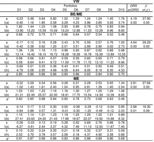
The results with the US data and portfolios based on the BE/ME index show that the models are not able to capturate the returns of portfolios; intercepts are signiﬁcant in most regressions and particularly high in the CAPM model. As a consequence, the null is rejected in both tests. The FF model is consistently better than the CAPM in terms of adjusted R2_{, with improvements around} ₂₀_percentage

points. One can also observe that the intercept point estimates increases from the lowest to the highest decile.

The estimations based on the ME index portfolios show similar results. The null of jointly zero intercepts is rejected in both tests. In fact, the null is rejected in the

13_{Málaga and Securato (2004) reach similar results, although they do not perform all the exercises}

(26)

CAPM because of portfolios D4 and D10. If the model is the FF, it is not rejected at5% using the GMM test. The increasing pattern of intercepts’ point estimates is also present in the CAPM model but not in the FF.

Diﬀerently from the Brazilian case, theβs of the portfolios BE/ME and ME are all greater than one in the CAPM model, but are less than 1 in portfolios D5-D10 if estimation includes the HML and SMB factors.

Table VI

Intercept Tests and Time Series Regression of Portfolios BE/ME and ME (NYSE, AMEX and Nasdaq)

The estimated equation is Ri,t−Rf,t =ai+bi(Rm,t−Rf,t) +siSM Bt+hiHM Lt+εt,i. t() is

the t-statistics of the OLS regressions. p(GRS)andp(χ)correspond to the p-values of the statistics GRS andχ described in the last section. The market portfolio is the value-weighted and T-Bill is the risk free rate. There are 92 monthly observations between January 1999 and August 2006.

GRS

D1 D2 D3 D4 D5 D6 D7 D8 D9 D10 p(GRS)

a -0.23 0.48 0.64 0.82 1.02 1.29 1.24 1.24 1.45 1.76 4.19 37.90 t(a) -0.40 1.16 1.85 2.58 3.29 4.23 3.96 3.85 3.93 3.74 0.00 0.00

b 1.82 1.44 1.23 1.08 0.93 0.89 0.78 0.75 0.83 0.94 t(b) 13.90 15.20 15.59 15.09 13.24 12.88 11.03 10.28 9.96 8.85 0.68 0.72 0.73 0.71 0.66 0.64 0.57 0.54 0.52 0.46

a -0.17 0.12 0.16 0.28 0.43 0.70 0.59 0.57 0.76 1.00 4.64 29.29 t(a) -0.42 0.38 0.62 1.20 2.01 3.51 2.89 2.90 3.02 2.73 0.00 0.00

b 1.36 1.26 1.18 1.10 0.98 0.93 0.87 0.82 0.88 0.98 t(b) 13.14 16.42 18.10 18.72 18.28 18.28 16.78 16.39 13.89 10.55

s 0.58 0.66 0.61 0.57 0.59 0.59 0.60 0.65 0.71 0.79 t(s) 5.59 8.64 9.41 9.72 11.00 11.76 11.72 13.10 11.23 8.66 h -0.60 0.01 0.23 0.36 0.43 0.41 0.51 0.50 0.49 0.51 t(h) -4.79 0.08 2.95 4.98 6.58 6.64 8.05 8.19 6.30 4.53 0.85 0.86 0.86 0.86 0.85 0.86 0.83 0.84 0.80 0.70

a -0.22 0.29 0.34 0.56 0.28 0.31 0.29 0.53 0.65 1.34 2.81 27.66 t(a) -1.02 1.43 1.61 2.40 1.04 0.95 0.81 1.39 1.40 2.54 0.00 0.00

b 1.03 1.03 1.23 1.16 1.16 1.30 1.27 1.25 1.29 1.06 t(b) 21.31 22.49 25.57 22.00 18.91 17.75 15.54 14.39 12.39 8.85 0.83 0.85 0.88 0.84 0.80 0.78 0.73 0.69 0.63 0.46

a -0.14 0.17 0.12 0.30 0.00 -0.08 -0.29 -0.12 -0.04 0.85 2.66 16.30 t(a) -0.84 0.88 0.57 1.31 -0.01 -0.30 -1.20 -0.49 -0.12 2.03 0.01 0.09

b 1.15 1.14 1.31 1.23 1.19 1.25 1.25 1.22 1.21 0.89 t(b) 27.41 23.60 24.93 21.43 17.98 18.67 20.07 19.92 15.88 8.32 s -0.26 -0.03 0.13 0.19 0.28 0.50 0.69 0.76 0.88 0.78 t(s) -6.27 -0.61 2.44 3.37 4.32 7.48 11.13 12.50 11.67 7.40 h 0.10 0.22 0.24 0.25 0.21 0.18 0.33 0.37 0.31 0.09 t(h) 2.03 3.70 3.78 3.57 2.58 2.18 4.37 4.92 3.38 0.68 0.91 0.87 0.89 0.86 0.83 0.86 0.88 0.89 0.86 0.69

(27)

4.2 Risk Premium

This section presents the estimates of equations (1) and (3) by GMM and ITNL-SUR methods. In the GMM case, the covariance function is estimated using the Parzen weighting function following Andrews (1991), who argues it is preferable over the Bartlett window, and, according to Ogaki (1993), it is computationally more convenient than the quadratic option.

The choice of the bandwidth is more critical than the choice of the weighting function (see Hall (2005)). For this reason, we estimate the model with 3 distinct bandwidths: none,1and4. If the series are uncorrelated, then the bandwidth should be zero. Hall (2005) suggests setting it equal to T13 ' 4 because it minimizes the mean square error of the covariance estimator. Finally, we also set the the bandwidth equal to 1 because the analysis of the series in Table II has shown that onlyﬁrst-lag correlations are statistically signiﬁcant.

The tables show the parameters estimated by GMM at the first stage, using the identity as weighting matrix - GMM1 - and the inverse of the long run covariance matrix as weighting matrix, iterated until convergence - GMM IT. Monte Carlo simulations show that when the sample is small, GMM estimates are better if the objective function is iterated until convergence (Ogaki (1993)). The argument for presenting GMM1 is as follows. When one groups portfolios according to financial characteristics, the weights are the same for every asset. If the weighting matrix is the statistical optimal, the economic content of the covariance matrix is lost (see Yogo, 2006, Cochrane, 2005). Therefore, by comparing the parameters of the GMM1 we are able to compare results from distinct, economic based, specifications. On the other hand, estimates obtained in GMM IT have nicer statistic properties. The estimates based on the identity weighting matrix and one iteration are similar to those obtained by OLS. The estimates based on the identity weighting matrix itered until convergence are similar to those obtained by GLS14_.

The portfolios used in the estimations are those deﬁned by the BE/ME and ME criteria. Moreover, we repeat the exercise using 44 stocks without any kind of grouping (44IBOV). In doing that, we avoid the criticism of Lewellen, Nagel and Shanken (2006). They argue that theβs are correlated with the other indexes.

Before going on, one should choose to include or not a constant, λ0, in the model

(1) and (3) (λ0 stands for the exceptional return beyond the excess return of the asset

with respect to the risk free rate). This turned out to be crucial in our estimates since it changed sensibly the results. Such a phenomenum is also present in the US data

14_{The estimate in two stages by OLS, GLS and WLS as suggested by Shanken and Zhou (2007)}

(28)

and is often disregarded in studies. As a matter of fact, Lewellen, Nagel e Shanken (2006) show that recent successful articles in explaining the cross-sectional variability of returns, such as Lettau and Ludvigson (2001) and Yogo (2006), present huge estimates forλ0, contradicting theory. Following economic arguments, we impose the

intercept to be null; the appendix presents the estimation under the less restrictive speciﬁcation for portfolios ME using Brazilian data. As can be seen, the inclusion of the constant lead to negative risk premium and high positive intercepts estimates.

Table VII presents the estimates for the 3 sets of portfolios (panels BE/ME, ME and 44IBOV) for Brazilian data. The CAPM model presented a positive market risk premium for all variants, except in the case 44IBOV with 4 lags, where the model failed to converge. In the cases the coefficient were significantly different from zero (ITNLSUR for ME and 44IBOV portfolios), the market risk premium in annual terms is about 6.5% a very plausible and generally agreed figure in the private market.

When the SMB and HML factors are included in the model, the risk premium is still signiﬁcant in the ITNLSUR method (ME and 44IBOV) at the same magnitude. Using the GMM method, the point estimates hardly resemble the time series means, possibly only on the ME portfolios. The estimates of the SMB premium, λsmb,

approximates the time series mean around0,99%in the portfolios BE/ME according to the GMM method. The HML premium, λhml, is negative and approximates the

time series mean around −0,79% in portfolios ME. However, GMM delivers non signiﬁcant coeﬃcients and, in this sense, agrees with time series means estimates.

Table VII

Cross-Sectional Regressions.

Econometric model: E[Ri,t−Rf,t] =λmβi+λssi+λhhi. In the GMM1,WT =I. The GMM IT

(29)

MAE Time Series 0.35 0.39 0.99 1.49 -0.79 -0.87

GMM 1 0 lag 1.23 1.22 0.43

GMM IT 0 lag 1.15 1.18 10.90 0.28 0.45 GMM IT 1 lag 1.09 1.07 10.88 0.28 0.46 GMM IT 4 lags 0.98 0.96 13.01 0.16 0.49

ITNLSUR 0.43 1.39 0.63

GMM 1 0 lag 0.53 0.53 1.05 0.44 0.19 0.10 0.22 GMM IT 0 lag 0.47 0.47 1.07 0.82 0.12 0.08 6.45 0.49 0.22 GMM IT 1 lag 0.60 0.58 1.03 0.80 0.14 0.10 6.19 0.52 0.22 GMM IT 4 lags 1.31 1.25 0.73 0.61 0.34 0.26 6.02 0.54 0.50 ITNLSUR 0.04 0.10 0.39 0.33 0.66 0.57 0.51

GMM 1 0 lag 1.15 1.14 0.32

GMM IT 0 lag 1.46 1.51 17.74 0.04 0.41 GMM IT 1 lag 1.25 1.28 17.20 0.05 0.34 GMM IT 4 lags 0.55 0.60 19.85 0.02 0.43

ITNLSUR 0.56 2.77 0.43

GMM 1 0 lag 0.96 1.02 0.44 0.41 -0.58 -0.29 0.32 GMM IT 0 lag 0.93 1.00 0.17 0.17 -0.45 -0.25 15.39 0.03 0.31 GMM IT 1 lag 0.84 0.89 0.19 0.18 -0.62 -0.33 15.09 0.03 0.34 GMM IT 4 lags 0.43 0.46 0.58 0.64 -1.25 -0.74 18.39 0.01 0.51 ITNLSUR 0.62 2.86 -0.54 -0.70 -0.21 -0.14 0.59

GMM 1 0 lag 0.86 0.90 1.15

GMM IT 0 lag 1.26 1.38 77.37 0.00 1.17 GMM IT 1 lag 1.09 1.22 84.53 0.00 1.15 GMM IT 4 lags -1.98 -4.88 569.61 0.00 2.75

ITNLSUR 0.51 5.13 1.20

GMM 1 0 lag 0.94 1.01 -1.28 -1.32 -0.73 -0.61 1.12 GMM IT 0 lag 0.87 0.95 0.40 0.50 -1.76 -1.65 69.16 0.00 1.68 GMM IT 1 lag 0.74 0.82 0.21 0.28 -1.45 -1.39 77.42 0.00 1.54 GMM IT 4 lags -1.10 -2.41 2.25 6.31 -1.40 -2.67 516.68 0.00 2.38 ITNLSUR 0.56 5.30 -0.30 -0.66 -1.52 -2.78 1.04

44IBOV Method

BE/ME

ME

χ p( )χ ( m)

tλ

m

λ λsmb t(λsmb) λhml t(λhml)

When comparing both models in terms of mean absolute error (MAE), the great-est improvement occurs in the BE/ME portfolios, where the error is reduced from 0.43% with the CAPM especiﬁcation to 0.22% with FF. There is only a tiny im-provement in the 44IBOV portfolios, decreasing from 1.15% to 1.12%, although the reduction is greater in the ITNLSUR estimation.

(30)

(BOVESPA) Average Monthly Returns (y-axis)× Predicted Monthly Return (x-axis)

Since Brazilian studies use short time series and a fewfirms, it is very difficult to compare the reliability of the results with those from the US, for instance. Therefore, we take the same period and grouping for the US data and compare the results with a longer sample. The portfolios are defined according the BE/ME criterium. The

ﬁrst sample, as usual, starts at January 1999 and ends at August 2006, hence it includes 92 months. The longer sample ends at the same date, but starts at July 1963, hence it includes 518 months.

Table VIII shows the results with the US data. In small sample, both CAPM and FF models estimate negative (except in GMM1) and insignificant market risk premium. The coefficient estimates of the FF model are significant. GMM IT with 1 and 4 lags shows significant coefficients for SMB and HML. The MAE reduced expressively using the FF model, although theχ test still rejects the null.

Table VIII

Cross-Sectional Regressions (NYSE/AMEX/Nasdaq) with 2 Samples: 92 and 518 Months.

Econometric Model: E[Ri,t−Rf,t] =λmβi+λssi+λhhi. In the GMM1,WT =I. The GMM IT

(31)

respectively, of the GMM objective function. MAE is the mean absolute error between the predicted value of the model and the observed value.

The larger sample shows more robust results. The FF model is not rejected and the ITNLSUR does not reduces the MAE with a larger sample. Interestingly, now only the HML coefficients are significantly different from zero, although still far from the time series mean. However, the fit using the larger sample is much better as Figure 2 shows. This result is responsible for the great success the FF model had in

(32)

(NYSE/AMEX/Nasdaq) Average Monthly Returns (y-axis)× Predicted Monthly Return (x-axis)

5 Conclusions

The intercept tests produce similar conclusions with respect to the CAPM and the 3 Factors Fama-French models. When the market portfolio proxy is the Ibovespa for Brazil, the intercepts with portfolios selected according to the BE/ME criterium are jointly null in both models, whereas under the ME criterium, the models are both rejected. However, other proxies for the market portfolio may change the results. If the proxies is either the MSCI Brazil or a portfolios with equal weights for the assets, then the models are not rejected at all.

Notwithstanding, the point estimates of the intercepts increases from the lowest to the highest portfolios as in the US case when portfolios selected according to the BE/ME criterium. Such an observation is independent of the proxy for the market portfolio. Possibly this reﬂects the presence of a value-premium in the Brazilian data, as the descriptive statistics already showed. The phenomenum does not occur to portfolios chosen by the ME criterium.

(33)

CAPM model on the BE/ME portfolios: mean absolute error - MAE - falls from 0.43% to 0.22% per month. On the other hand, both models perform similarly on the ME portfolios, around 0.32% of monthly MAE. In the case of the 44IBOV data set, the multifactorial model is marginally superior to the CAPM (1.15% to 1.12%). The US data are more conclusive, and justiﬁes the success of the FF model relatively to the CAPM (MAE from 0.67% to 0.08% in the BE/ME portfolios). With US data, anomalies are sharper than Brazilian data, what really makes the CAPM performance in the US to be unsatisfactory. Indeed, in the more robust results with the larger sample, the FF model was not rejected whereas the CAPM was. In the reduced sample, the same qualitative conclusion is reached, although the signiﬁcance of the parameters worsens.

The risk premium, in general, was not statistically significant with Brazilian data. However, when the premium was significant, it was positive; the ITNLSUR point estimate indicates a premium of 6.5% per year, in line with private market usually agreed expectations, whereas the time series mean pointed to 4.25% per year although not statiscally significant. The factor premia SMB and HML were both statistically non significant, even when accounting for serial correlation. Using the US data, the premia SMB and HML were significants with the small and large samples, respectively, and the market premia was zero.

(34)

6 References

Andrews, D. W. K. (1991): “Heteroskedasticity and Autocorrelation Consistent

Covariance Matrix Estimation,” Econometrica, 59(3), 817—858.

Banz, R. W.(1981): “The Relationship between Return and the Market Value of

Common Stocks,” Journal of Financial and Quantitative Analysis, 14, 421—441.

BASU, S.(1977): “Investment Performance of Common Stocks in Relation to their

Price-Earnings Ratios: A Test of the Eﬃcient Market Hypothesis,” Journal of

Finance, 32, 663—682.

Black, F.(1972): “Capital Market Equilibrium with Restricted Borrowing,”

Jour-nal of Business, 75(3), 444—455.

Black, F., M. Jensen, and M. Scholes (1972): “The Capital Asset Pricing

Model: Some Empirical Tests,” in Studies in the Theory of Capital Markets, ed. by M. C. Jensen, pp. 79—121. Praeger, New York.

Blume, M., and I. Friend (1975): “The Asset Structure of Individual Portfolios

with Some Implications for Utility Functions,” Journal of Finance, 30, 585—604.

Bonomo, M.(2002): Financas Aplicadas Ao Brasil. Editora FGV, RJ.

Breeden, D. T. (1979): “An Intertemporal Asset Pricing Model with Stochastic

Consumption and Investment Opportunities,”Journal of Financial Economics, 7, 265—296.

Burmeister, E., and M. B. McElroy (1988): “Arbitrage Pricing Theory as a

Restricted Nonlinear Multivariate Regression Model,” Journal of Business and

Economic Statistics, 6(1), 29—42.

Campbell, J. Y., A. Lo, and C. MacKinlay (1997): The Econometrics of

Fi-nancial Markets. Princeton University Press, Princeton.

COSTA Jr., Newton, R. L., and E. Lemgruber (2000): Mercado de Capitais:

Analise Empirica No Brasil. Editora Atlas, SP.

Fama, E. F., and K. R. French (1992): “The Cross-Section of Expected Stock

Returns,” Journal of Finance, 47(2), 427—465.

(1993): “Common risk factors in the returns on stocks and bonds,”Journal

(35)

(1995): “Size and Book-to-Market Factors in Earnings and Returns,”

Jour-nal of Finance, 50, 131—156.

(1996): “Multifactor Explanations of Asset Pricing Anomalies,” Journal of

Finance, 51(1), 55—84.

Fama, E. F.,and J. MacBeth(1973): “Risk, Return and Equilibrium: Empirical

Tests,”Journal of Political Economy, 81, 607—636.

Gibbons, M. R., S. A. Ross, and J. Shanken(1989): “A Test of the Eﬃciency

of a Given Portfolio,” Econometrica, 57(5), 1121—1152.

Hall, A. R.(2005): Generalized Method of Moments. Oxford University Press, New

York, NY.

Hansen, L. P.(1982): “Large Sample Properties of Generalized Method of Moments

Estimators,” Econometrica, 50(4), 1029—1054.

Harvey, C., and C. Kirby (1995): “Analytic Tests of Factor Pricing Models,”

Working Paper.

Lewellen, Jonathan, S. N., and J. Shanken (2006): “A Skeptical Appraisal

of Asset-Pricing Tests,” NBER Working Paper.

Lintner, J. (1965): “The Valuation of Risky Assets and the Selection of Risky

Investments in Stock Portfolios and Capital Budgets,” Review of Economics and

Statistics, 47, 13—37.

Lucas, Jr., R. E.(1978): “Asset Prices in an Exchange Economy,”Econometrica,

46, 1426—14.

MacKinlay, A. C., and M. P. Richardson(1991): “Using Generalized Method

of Moments to Test Mean-Variance Eﬃciency,”Journal of Finance, 46(2), 511—27.

Malaga, F. K., and J. R. Securato (2004): “Aplicação Do Modelo de Três

Fatores de Fama e French No Mercado Acionário Brasileiro - Um Estudo Empírico Do Período 1995-2003,” in EnAnpad. Anpad.

Markowitz, H. M.(1952): “Portfolio Selection,”Journal of Finance, 7(1), 77—91.

Merton, R. C. (1973): “An Intertemporal Capital Asset Pricing Model,”

(36)

Ogaki, M. (1993): Generalized Method of Moments: Econometric

Applica-tionschap. 17, pp. 455—485, Handbook of Statistics, Vol 11. Elsevier Science

Pub-lishers.

Roll, R. W.(1977): “A Critique of the Asset Pricing Theory’s Tests,” Journal of

Financial Economics, 4, 129—176.

Rosenberg, B., K. Reid, and R. Lanstein (1985): “Persuasive evidence of

market ineﬃciency,”Journal of Portfolio Management, 11, 9—17.

Ross, S. A. (1976): “The Arbitrage Theory of Capital Asset Pricing,” Journal of

Economic Theory, 13, 341—360.

Shanken, J., and G. Zhou(2007): “Estimating and Testing Beta Pricing Models:

Alternative Methods and their Performance in Simulations,” Journal of Financial

Economics, 84, 40—86.

Sharpe, W. F. (1964): “Capital Asset Prices: A Theory of Market Equilibrium

Under Conditions of Risk,” Journal of Finance, 19, 425—442.

Yogo, M. (2006): “A Consumption-Based Explanations of Expected Stock

Re-turns,” Journal of Finance, 61(2), 539—580.

7 Appendix

The appedix division follows the body text. Details regarding each section follows the text section titles.

7.1 Data Set and Portfolio Construction

7.1.1 Portfolios

Composition of ME Porftolios The ﬁrms were ordered according to their marke value (ME), and grouped in 10 portfolios (D1 the largest corporations, D10 the smallest corporations). Firms with more than one stock were kept in the same group with the same weight. The returns were equally weighted. Next table presents the composition of the portfolios in 2006, based on information released in December 2005.

Table A1

(37)

The data set contains 123 ﬁrms, whose stocks were traded in Bovespa between January 1999 and August 2006.

D1 D2 D3 D4 D5 D6 D7 D8 D9 D10

PETR TNLP BRKM SBSP ACES GLOB AVPL RHDS FJTA IENG VALE TMAR BRTP SDIA LIGT LEVE PEFX BOBR IGBR INEP BBDC CMET GOAU GUAR DURA CNFB ITEC FBRA HGTX TELB AMBV EMBR VIVO NETC TMCP CLSC EBCO CRIV MTSA TRFO ITAU CSNA EBTP BFIT PTIP PQUN ROMI FLCL TNCP TEKA BBAS CMIG VCPA KLBN TMGC RSID BRIV BRGE VAGV MWET UBBR BESP BRTO PRGA ALPA MYPK FRAS ETER PNVL BCAL

ITSA USIM TCSL SUZB CTNM COCE DXTG RPAD MNDL LIXC TLPP ARCZ LAME CGAS CESP CEPE ASTA LIPR PLAS ESTR ELET TBLE CPSL FFTL UNIP ELEK PLTO EMAE MGEL SULT ARCE CRUZ WEGE CEEB PMAM RIPI ILMD SGAS CGRA JBDU GGBR PCAR CPLE CBEE RAPT BSCT FESA PNOR BDLL MNPR

DPPI POMO MAGS

BE/ME The ﬁrms were ordered according to the size of the BE/ME index, from the lowest to the highest and grouped in 10 portfolios (D1toD10). Firms with more than one stock were kept in the same group with the same weight. We have excluded ﬁrms with negative book equity, they were grouped in portfolio VX. Next table shows the composition of the portfolios in 2006, based on information released in December 2005.

Tabela A2

Portfolios Composition BE/ME in December 2005

VX D1 D2 D3 D4 D5 D6 D7 D8 D9 D10

BCAL BSCT AMBV ARCZ ALPA ARCE BRKM AVPL ACES ASTA BDLL BOBR CMET BBDC BESP BBAS CNFB CEEB BRTO CEPE BRGE CESP ESTR CPSL CGAS BFIT CBEE DURA COCE BRTP CGRA BRIV ELET MWET CRUZ EMBR CMIG CSNA DXTG LIGT CLSC CRIV CPLE EMAE PMAM GUAR FFTL ELEK GLOB GOAU POMO ETER CTNM EBCO FJTA

TEKA HGTX FRAS GGBR LIPR ILMD PQUN FBRA DPPI FESA IENG VAGV LAME ITAU ITSA MTSA ITEC ROMI IGBR EBTP JBDU INEP MYPK LEVE PCAR PEFX KLBN TMAR PTIP FLCL PLTO LIXC NETC PRGA PETR RIPI TMCP USIM RHDS MAGS PNOR MGEL RSID RAPT PLAS SDIA VIVO VCPA SUZB MNDL RPAD MNPR TBLE UBBR TLPP TCSL TRFO PNVL SBSP SULT VALE WEGE TNLP TMGC UNIP SGAS TNCP TELB

7.1.2 Factors

(38)

terms of market value, and the other, the remaining 62. The firms were again split into 3 groups according to the size of the index BE/ME: H (high), M (medium) and L (low). The extreme groups counted each for 30% of the firms, and the medium group for 40% of thefirms. The market value was calculated by multiplying the free

ﬂoat stocks times the price stocks.

The intersection of these two groups makes 6 sets of stocks: HB,HS,MB, MS,

LB andLS, which weighted by the market value of eachﬁrm generate 6 portfolios. The composition of these stocks is rebalanced yearly on the basis of the Balance sheet corresponding to December of the previous year, except the initial portfolio based on January 1999. Firms with negative equity were excluded. The next table shows the last composition ofﬁrms in each group followed by a descriptive statistics.

Table A3

Fama French Portfolios for SMB and HML in December 2005

HB HS MB MS LB LS

ACES ASTA ALPA AVPL AMBV BSCT CESP BDLL ARCE CLSC ARCZ ELEK CPLE BRGE BBAS CNFB BBDC FRAS CTNM BRIV BRKM COCE BESP HGTX EBTP CEPE BRTO DXTG BFIT LEVE ELET CGRA BRTP ETER CGAS MYPK SBSP CRIV CBEE FBRA CMET PLAS DPPI CEEB IGBR CMIG RSID EBCO CSNA ILMD CPSL EMAE DURA ITEC CRUZ FESA GLOB LIPR EMBR FJTA GOAU MTSA FFTL FLCL KLBN PEFX GGBR IENG LIGT PNVL GUAR INEP PTIP POMO ITAU JBDU SDIA PQUN ITSA LIXC SUZB RHDS LAME MAGS TCSL RIPI NETC MGEL TMAR ROMI PCAR MNDL TMCP TRFO PETR MNPR TMGC PRGA PLTO TNLP RAPT PNOR UNIP TBLE RPAD USIM TLPP SGAS VCPA UBBR SULT VIVO VALE

TELB WEGE

TNCP

Table A4

Descriptive Statistics - Fama French Six Portfolios: BOVESPA and NYSE/AMEX/Nasdaq between January 1999 and August 2006

The Capm and Fama-French models in Brazil: a comparative study

Fundação Getulio Vargas

Escola de Economia de São Paulo

The CAPM and Fama-French Models in Brazil: A

Comparative Study

Fernando Daniel Chague

Fernando Daniel Chague

The CAPM and Fama-French Models in Brazil: A

Comparative Study

The CAPM and Fama-French Models: A

Comparative Study

Fernando Daniel Chague

Escola de Economia de São Paulo

Fundação Getulio Vargas

November 22, 2007

Contents

1

Introduction

2

Data Set and Portfolios Construction

2.1

Data Set

2.2

Portfolio Construction

2.3

Market Portfolio and Factors

3

Theory and Econometric Tests

3.1

Test of Intercepts

3.2

Risk Premium

4

Empirical Analysis

4.1

Intercept Tests

4.2

Risk Premium

5

Conclusions

6

References

7

Appendix

7.1

Data Set and Portfolio Construction