A Structuralist Philips Curve Nelson Barbosa*
Abstract: this paper presents a structuralist model of the Philips curve and applies it to the US and Brazilian economies. The theoretical model starts from a simple markup rule to build a Philips curve based on the assumptions that firms have a desired rate of profit and wokers have a target real wage. Inflation expectations are modeled in terms of current inflation and the governments’ target, and the model shows that relative prices can have both a short-run and long-run influence on inflation. When applied to the US, the structuralist Philips curve results in a nonlinear model in which there are two steady states for inflation, and where the wageshare of income becomes the main instrument to drive inflation to the governments’ target. When applied to Brazil, the structuralist Philips curve reveals a nonlinear relationship between long-run inflation and the real exchange rate, so that the same inflation target can be consistent with more than one value of the exchange rate. The main conclusion of the paper is that a structuralist specification of the Philips curve is a useful instrument to model many macroeconomic topics as well as alternative theoretical closures.
Keywords: inflation, Philips curve, structuralist macroeconomics JEL code: E11, E12 and E31
*
Introduction
The Philips curve is an indispensable part of any macroeconomic model. Many works have been done on the link between inflation and economic activity since the first proposition of the Philips curve in the 1950s, as related by Gordon (2009). In general terms the current mainstream approach to the topic specifies inflation in terms of three components: expected inflation, demand pressures and supply shocks. The modeling varies across authors but there is a common view in the mainstream literature that agents have rational expectations about inflation and that there is only one level of economic activity, be it the non-accelerating-inflation rate of unemployment or rate of capacity utilization, consistent with stable inflation. The ob*ective of this paper is to present an alternative formulation of the Philips curve based on the structuralist
approach to macroeconomics (Taylor 2004). The starting point of the structuralist Philips curve is similar to the one adopted in some mainstream models, a markup rule for price determination, but its underlying assumptions follow the post-Keynesian and Sraffian views about effective demand and income distribution. The result is a versatile model in which there may be more than one level of economic activity consistent with stable inflation, an inflation curve, and where income distribution plays an important part in inflation dynamics. The structuralist Philips curve also allows relative prices to have a long-run impact on inflation through its effect on the rate of profit and income distribution. In this way a structuralist specification of the Philips curve opens the
possibility of multiple equilibria as well as of a long-run link between inflation and growth. The analysis is organized in three sections. The first section presents the
theoretical model and discusses its main implications. The second section applies the model to the US economy and shows how indexation and income distribution may impact inflation in the long-run. The third section applies the model to Brazil and shows how a key relative price, the real exchange rate, can have a long-run impact on inflation. The final section concludes the analysis with observations on other lines of research based on the structuralist approach to the Philips curve.
Theoretical Model
Assume that prices are fixed through a markup rule over unit production cost as follows:
= ( + ), (1)
where is the price level, the markup multiplier, the nominal wage, the price of non-labor inputs, the labor-output ratio, and the ratio of non-labor inputs to output. The economic logic of (1) is that firms determine prices to obtain a desired markup over unit production costs, which in its turn is an instrument to obtain a desired rate of profit on physical capital. From (1) the rate of inflation is:
where is the growth rate of the markup, the share of labor in the cost of production, the wage inflation, − the growth rate of average labor productivity, the inflation rate of non-labor input prices, and the growth rate in the non-labor input-output ratio.
Next, in line with Structuralist or Sraffian models of income distribution, assume that the change in the markup follows an error-correction process in which the effective rate of profit on physical capital converges to the desired rate of profit by firms.1 More formally:
= ∗− (1 − − )( ⁄ ) , (3)
where is a nonnegative parameter, ∗ is the target rate of profit, the wageshare of output, the relative price of the non-labor input, the output-capital ratio and the relative price of the non-labor input. In structuralist macroeconomics the target rate of profit is usually a function of the real interest rate, the monopolistic power of firms, the risk of investing in physical capital and other institutional and behavioral variables.
Moving to wage inflation, assume that workers set their claims as the sum of expected inflation and a desired growth rate of the real wage, that is:
= + ( , ). (4)
The economic logic behind (4) is that workers have a target for the real wage, which in its turn is a function of both the level of economic activity and the state of income
distribution. On one side, as usual in mainstream models, we assume that a high level of economic activity increases the workers’ bargaining power and pushes wage inflation up. On the other side, from a structuralist perspective, we also assume that a low wageshare means that only a small part of labor productivity is being paid to workers, which also pushes up wage inflation. In terms of (4) these two assumptions mean that is a positive function of and a negative function of .2
By analogy with (4), define the inflation rate on non-labor inputs simply as expected inflation plus a relative-price term, that is:
= + ", (5)
where by definition # represents the expected change in the relative price of non-labor inputs. The modeling trick of (5) is to use the very own definition of a supply shock to
1
Many mainstream and heterodox models assume a fixed markup and focus the analysis *ust on the wageshare. We do not do this here because the rate of profit and not the markup is the main variable for firms. As we will see later, the change in the markup introduces interesting dynamics in the model. 2
define non-labor input inflation in a way that isolates changes in relative prices in an independent term.
After some algebraic operations we can rewrite inflation as:
= + ∗− (1 − − )( ⁄ ) + ( + ) + (1 − )( + "). (6)
In terms of the literature on the Phillips curve, (6) resembles Gordon’s (1982) “triangle” model since it specifies inflation in terms of an “expected” component, a “demand” component, and “supply-shock” component.3 Despite this similarity, there are two main differences between the mainstream approach to inflation and the structuralist approach presented in (6): the possibility of multiple equilibria and the impact of relative prices on inflation. Let us see each point separately.
First, note that since the wageshare of income enters as an independent determinant of inflation in the structuralist version of the Phillips curve, we can have more than one level of economic activity consistent with stable inflation in (6). More formally, if we define the income-capital ratio as a proxy of capacity utilization, then there is a “curve” of points in the × plane consistent with = . So, in contrast to mainstream models, according to (6) there may be more than one value of capacity utilization consistent with stable inflation.4
Second, the markup dynamics depend not only on the wageshare and the level of economic activity, but also on the level of some key relative prices. More formally, from (6) inflation depends on the relative price of the non-labor input and the relative price of capital. As a result, inflation depends both on the temporary impact of changes in relative prices and the long-run level in which relative prices stabilize. The economic intuition of this result is that a particular set of relative prices may be more or less inflationary than another because of its impact of the rate of profit. As a result, the long-run values of relative prices matter because they affect the state of income distribution and the level of economic activity necessary to stabilize inflation.
To complete the model, assume that expected inflation is a positive function of current inflation and the inflation target set by the government.5 On the one side the logic behind this assumption is that agents expect some inertia in inflation, so that
current inflation has a positive impact on expected inflation. On the other side agents also expect that macroeconomic policy in general, and monetary policy in particular, will drive
3
The expected component is naturally the expected inflation in the right-hand side of (6). The demand component is the sum of the growth rates of the markup and the wageshare. The supply-shock component is the residual.
4
One common characteristic of structuralist models is that capacity utilization is stable but not necessarily unique in the long-run. For the heterodox literature on growth and distribution, see: Marglin (1984), Dutt (1990), Taylor (1991 and 2004) and Foley and Michl (1999).
5
inflation to the target set by the government. The simplest way to represent these two assumptions is to define:
= & + (1 − &) ∗, (7)
where 0 < & < 1 represents the degree of inflation inertia and ∗ is the agents’ expectation about the government’s inflation target.6 From (6) and (7) we have:
= ∗+ ( )
)*+, -( ∗, , , , , , ) + .( , #) , (8)
where naturally - = ∗− (1 − − )( ⁄ ) + ( + ) and . = (1 − )( +
"). The main economic meaning of (8) is that, in the absence of supply shocks (. = 0), inflation is equal to the government’s target as long as macroeconomic policy drives effective demand and income distribution to a point in which there are no excessive pressures on inflation (- = 0).7
Finally, let’s see the main theoretical implications of (8). First considering the level of economic activity, we have:
/0 /1= (
) )*+, 2−
3()*4*56)
57 +
/8 /19,
so that inflation is pro-cyclical as long as the positive impact of economic activity on the workers’ target real wage growth predominates over its positive impact on the rate of profit.
Second, considering income distribution, we have: /0
/4= ( ) )*+, 2
31 57+
/8 /49,
which can be either positive or negative depending on how the workers’ target real-wage growth responds to the wageshare.
Third, focusing on the link between inflation and growth, assume that supply shocks are equal to zero in the long-run. If the wageshare is stable ( + = 0) and firms obtain their desired rate profit ( = 0), then inflation is equal to the governments’ target. Since in the long run the output-capital ratio is usually stable, the stability of the markup gives us the long-run growth rate of the economy in terms of income distribution,
6
It should be noted that & can be a positive function of inflation, so that high inflation tend to increase inflation inertia. As we will see in the next section, when we work in discrete time this assumption gives rise to two equilibrium points, one stable and one unstable.
7
the desired rate of profit, the relative prices of capital the non-labor input, and the investment-GDP ratio. More formally, by definition the steady-state value of is
= (: + ;) <⁄ ,
where : is the growth rate of income, ; the rate of capital depreciation and < the investment-GDP ratio.8 So, the stability of the markup means that:
: = < ( =∗57
)*4*56>, − ;.
In economic terms we have at least two ways to read the equation above. The desired rate of profit and the stable wageshare determine economic growth for a given set of relative prices and technological parameters, or economic growth and the desired rate of profit determine the wageshare for a given set of relative prices and technological parameters. But so much for theory, let us now see two possible applications of our theoretical framework.
Inflation inertia: an application to the US economy The discrete-time version of (6) can be defined as:
? = ? + -? + .?+ @?, (9)
where - and . have the same meaning of the previous section and @? is a residual term that represents all second-order effects that inevitably appear when one works in discrete time. Our assumption about expectations can be represented as:
? = & ?*)+ (1 − &) ?∗, (10)
so that our Phillips curve can be rewritten as
Δ ? = (1 − &)( ?∗− ?*)) + -?+ .?+ @?. (11)
The intuitive meaning of (11) is that the change in inflation can be modeled as a result of four terms: (i) an error-correction term according to which inflation converges to the target set by the government; (ii) a demand-distribution term that captures the influence of capacity utilization and income distribution on inflation; (iii) a supply-shock term that captures the influence of changes in the productivity and relative price of non-labor inputs on inflation; and (iv) a residual term that represents second-order effects.
8
It should also be noted that if the inertia coefficient & is a function of past
inflation, then we have two possible steady states for inflation. More formally, assume for simplicity that & takes a linear form for the economic relevant values of inflation:9
&? = &A+ &) ?*). (12)
Then, in the absence of supply shocks and residual effects and assuming that
macroeconomic policy eliminates demand and distributive pressures on inflation, there are two steady states for inflation: ?∗ and −&A/&). The lower value of these two roots is the stable equilibrium point and the higher value is the unstable one.
Now let us apply the model to the US. Using the data from the Bureau of Economic Analysis, our sample consists of quarterly time series for the following variables:
1. Inflation: measured by the first difference of the log of the price index of personal consumption expenditures (PCEP).
2. Wageshare: measured by the ratio of labor compensation to gross domestic income (S_LCOM).
3. Output gap (GAP): measured by the difference between the log of real GDP and its long-run trend, with the latter defined as the Hodrick-Prescott moving average of GDP with a smoothing factor of 1600.
4. Supply-shock: measured by the first difference of log of the price index of oil imports (POIL) taken from the US balance of payments.
5. Crash of 2008-09: a dummy variable (DCRASH08) that equals one in the last quarter of 2008 and first quarter of 2009 to represent the impact of the recent financial crisis.
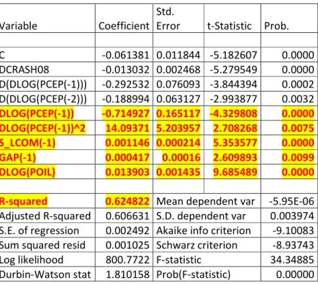
The period under analysis is 1967-2010 and, following (11), we estimate the model for the change in inflation. Table 1 below presents the econometric results of our model. We can re*ect the null hypothesis for all estimated coefficients at 2% of statistical significance and the regression explains 62% of the sample variation of the dependent variable. The variance-covariance matrix was estimated using the Newey-West method to deal with heteroskedasticity and autocorrelation.
TABLE 1 HERE
In economic terms the coefficients indicate that inflation is pro-cyclical and that an increase in the wageshare pushes up inflation. As expected, changes in price of oil have a positive impact on inflation and, more importantly, the results also indicate a
non-linearity in the US economy during the period under analysis. More specifically, for a given value of the other explaining variables, the change in inflation seems to be a concave-up function of past inflation, so that there are two equilibrium points for
9
inflation. To illustrate this, figure 1 below show the change in inflation as a function of past inflation for different values of the wageshare. The underlying assumption is that the supply shock, the output gap and the residual term are all equal to zero to focus the analysis *ust on the impact of income distribution on the long-run value of inflation.
FIGURE 1
According to figure 1, in the absence of supply and demand shocks the US annual inflation is stable at 1.7% when the wageshare is equal to 56% of gross domestic income. If the wageshare rises to 60%, then the stable annual inflation rate moves to 3.5%. The economic logic of this result is that a higher wage share pushes up inflation because it reduces the rate of profit. So, assuming that the government has a pre-determined inflation target, macroeconomic policy has not only to zero the output gap, but also to change income distribution until the wageshare is consistent with the inflation target. Since the output gap is defined in a way that it always tends to zero in the long-run, at the end of the day the wageshare and the growth rate at which the output gap equals zero become the “instrument” variables to meet the inflation target.10 In other words, macroeconomic policy “closes” the model by determining the long-run inflation target, which in its turn set the non-accelerating-inflation wageshare according to the curve shown in figure 1.
The econometric results also indicate that US annual inflation tends to become unstable when it reaches 18% for a wageshare of 56%, or 16% for a wageshare of 60%. The economic logic is that the higher the inflation the more rigid it becomes downwards. As inflation goes up, the economy reaches a point in which inflation stabilizes, the “high-inflation” equilibrium, and beyond which the economy enters in the path to hyper-inflation.
Exchange rate and inflation: an application to the Brazilian economy
In the previous section we modeled supply shocks as changes in the price of oil because this has usually been the main source of “exogenous” price disturbances in developed economies. When we move to developing economies the real exchange rate is usually the main source of exogenous shocks to inflation because these economies do not issue international-reserve currencies. With this idea in mind, we will now apply out theoretical model to the Brazilian economy.
From (11) we can assume that a change in the real exchange rate affects inflation by the change in the relative price of non-labor inputs. As expected in cost-push models of inflation, a depreciation of the domestic currency accelerates inflation and an
10
appreciation decelerates it.11 Moreover, as long as the economy is not in the unstable-inflation region in which inertia becomes explosive, the impact of a depreciation of the domestic current is temporary. As long as the real exchange rate and relative prices stabilize at new levels the supply shock goes back to zero. But what about the permanent effect of the new relative prices? From our theoretical model the rate of profit depends on income distribution, which in its turn depends on the wageshare and some key relative prices as the real exchange rate.
To analyze the effect of the real exchange rate on long-run inflation assume that there are no supply shocks or residual disturbances in (11). Then the impact of the real exchange rate on inflation dynamics occurs through its influence on the long-run values of the wageshare, the relative price of non-labor inputs, the relative price of capital and the level of economic activity.
Considering first the wageshare, we can assume that is a negative function of the real exchange rate for two reasons. First, an increase in the real exchange rate pushes up the price of both tradable and non-tradable goods, with the former rising
proportionally more than the latter. Since wages usually do not keep up with prices, the result is a fall in the real wage, that is, a shift in income distribution against workers. Second, an increase in the real exchange rate also accelerates the growth rate of the tradable sector of the economy, which is usually the sector with the higher average labor productivity. As result, the change in relative price alters the composition of output and employment, which increases the average labor productivity and reduces the wageshare of income. In terms of our model these two assumptions can be represented as:
= A− )C, (13)
Where C is the real exchange rate and )> 0.
Moving to the other relative prices, the impact of the real exchange rate in the long-run is indeterminate a priori because it depends on weight of tradable and non-tradable goods in the composition of non-labor inputs and capital. Based on the
economic history of developing economies like Brazil, the real exchange rate usually has a positive impact on the relative prices of non-labor inputs and capital because a high share of these goods are imported. Based on this stylized fact, we can model relative prices as:
E= E,A+ E,)C, (14)
for F = G, H and where E,)> 0.
Finally, considering the level of economic activity, the impact of the real exchange rate on the income-capital ratio depends on the balance between its impact on domestic absorption and net exports. On one side, a high real exchange rate tends to reduce
11
domestic consumption and investment because it reduces the real disposable income of domestic agents. On the other side a high real exchange rate also increase net exports because it increases the competitiveness of domestic producers of tradable goods. The net impact is indeterminate a priori, it has to be closed empirically.
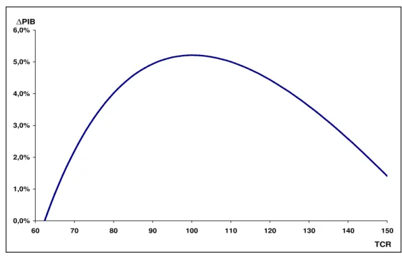
To make things more interesting, a recent study of the Brazilian economy found that the real exchange rate has a nonlinear impact on economic growth.12 The logic of this result is that initial condition matters, that is the impact of depreciation or appreciation of the domestic currency depends on the initial level of the exchange rate. The results indicate that if the real exchange rate is too low, a depreciation of the domestic currency accelerates growth because its negative impact on domestic absorption is more than compensated by its positive impact on net exports. By analogy, when the real exchange rate is too high the opposite happens and, therefore, there is an “optimal” level of the real exchange rate that maximizes the growth rate of the economy, as shown in figure 2.
FIGURE 2 HERE
The concave-down curve shown in figure 2 can be explained in many ways. It may be a result of macroeconomic policy that turns restrictive either when the real exchange rate is too low, to avoid excessive current-account deficits, or when the real exchange rate is too high, to avoid an acceleration in inflation. Alternatively, it may be the result of the market strategy of firms, since a reduction in the real exchange rate does not reduce net exports if domestic firms cut their markup, which in its turn is most probable if the initial markup was high due to an initially high real exchange rate. By analogy, the opposite happens when the initial real exchange rate is too low, so that we obtain the concave-down curve shown in figure 2.
Returning to inflation, for the specific purpose of our Philips curve it is sufficient to note that figure 2 means that the output-capital ratio can be modeled as:
= A+ )C − ICI, (15)
where I> 0.
Now, based on (13), (14) and (15), the growth rate of the markup becomes a nonlinear function of the real exchange rate. To see this, not that (3) can be rewritten as:
= ∗− J)*K4LM56,L>NMK4O*56,O>NP
57,LM57,OP Q ( A+ )C − IC
I). (16)
In mathematical terms (16) means that the growth rate of the markup, and therefore inflation itself, behaves approximately as 3rd-degree polynomial of the level of the real exchange rate. The economic meaning of this result is that inflation is relatively constant for moderate levels of the real exchange rate, but it varies substantially when the real
12
exchange rate is either too high or too low. For example, if )− ,) > 0, then inflation is a positive function of the real exchange rate when the real exchange rate is either too low or to high, but a negative function when the real exchange rate is at an intermediary level. The logic off this result is that too much appreciation or deprecation reduces the level of economic activity, which in its turn reduces the rate of profit and pushes up inflation. In contrast, for intermediary values of the real exchange rate the level of economic activity goes up and pushes down inflation through its influence on the rate of profit.
Moving to the Brazilian case, let us estimate a version of (11) in which the change in inflation is a 3rd-degree polynomial of the real exchange. The sample consists of quarterly observations of the following variables:
1. Inflation: the first difference of the log of consumer prices, according to the IPCA index.
2. Real exchange rate (RER): the real effective exchange rate estimated by the Central Bank of Brazil according the prices of Brazilian exports and the IPCA price index, this is an index number for which 1994=100.
3. Output gap (GAP): the difference between the log of industrial production and its long-run trend, with the latter defined as the Hodrick-Prescott moving average of GDP with a smoothing factor of 14400.
We did not introduce the wageshare as a separate explaining variable in the model because there is no quarterly series for such a variable available in Brazil. As an
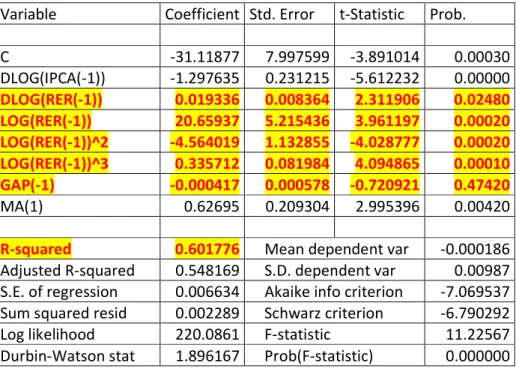
alternative and to control for autocorrelation, we modeled the error term of our model as a 1st order moving average process, which indirectly captures the fluctuations in the wageshare and other explain variables. The period under analysis is 1996-2011 and table 2 below presents the econometric results of the econometric model.
TABLE 2 HERE
As we did in the previous sections, the variance-covariance matrix of the error terms was estimated using the Newey-West method. The model explains 60% of the sample variance of the dependent variable. The coefficient on the change in the real exchange rate is positive and statistically significant at 5%. In economic terms this means that a depreciation of the domestic currency has a temporary positive impact on inflation, as one would expect from markup models. More importantly, all coefficients for the levels of the real exchange rate are statistically significant at less than 0,05%, which is a strong evidence that Brazilian inflation behaves as a 3rd-degree polynomial of the real exchange rate. In addition to this, the model also indicates that we cannot re*ect the null hypothesis that the coefficient on the output gap is equal to zero even at 10% of
exchange rate and the level of economic activity, which also confirms our previous assumption.13
Finally, to illustrate the long-run impact of the real exchange on inflation, assume that the real exchange rate is stable, that the output gap is zero and that there are other shocks to prices.14 Then, according to our results, inflation can be represented as shown in figure 3 below.
FIGURE 3 HERE
In economic terms, inflation is a positive function of the level of the real exchange rate when the real exchange rate is either too low (an index number below 80 in figure 3) or too high (an index number above 108 in figure 3). For intermediary values inflation becomes a negative function of the real exchange rate and, most importantly, in some cases the same inflation rate can be consistent with more than one value of the real exchange rate. In terms of macroeconomic policy this result means that there may be more than one equilibrium real exchange rate consistent with the same inflation target.
In comparison to the US case, where the wageshare defined the long-run rate of inflation for a zero output gap, in Brazil the real exchange rate functions as the main variable to “close” the Phillips curve. More specifically, given an inflation target, macroeconomic policy has not only to zero the output gap, but also to drive the real exchange rate to a point or an interval consistent with the governments’ ob*ective. To illustrate this point, figure 3 also shows the current upper and lower bounds of Brazil’s inflation target. From our econometric results there is a range of possible real exchange rates consistent with inflation being within the governments’ interval.15 So, as usual in structuralist macroeconomics, relative prices matter, but relative prices do not
necessarily constrain macroeconomic policy to a limited number of choices, provided that the government targets are adequate to the economy’s structure.
Conclusion
Structuralist macroeconomics takes a top-down approach in modeling economic problems. The starting point is usually an accounting identity to which behavioral functions and stylized facts are added to form a theoretical model. The models are usually versatile to be able to deal with the variety of economic structures and institutions that one finds in real-world economies. The model we presented in this paper follows the structuralist tradition and offers a flexible approach to model inflation dynamics in advanced and developing economies. The general principle is that prices are
13
In a separate regression, the output gap in Brazil seems to be a concave-down function of the real-exchange-rate during the period under analysis, as assumed in (15).
14
By analogy with what we did for the US, by definition the long-run output gap for Brazil is always zero. 15
determined by the conflicting claims on output, and that effective demand influences price determination through its impact on the rate of profit and the bargaining power of workers. In addition to these traditional features of Keynesian-Sraffian models, the Phillips curve presented in this paper also opens new ways to expand our analysis of inflation. First, as we modeled the US economy, the impact of inflation on markets’ expectations can result in multiple equilibria through endogenous indexation. More importantly, income distribution also becomes a crucial endogenous variable to make inflation coincide with the governments’ target. Second, as we modeled the Brazilian economy, relative prices matter for the long-run rate of inflation. A particular set of prices may be more inflationary than another, and there may also be multiple equilibria. The same inflation target can be consistent with alternative values of the exchange rate, which in its turn can result in different but stable growth rates.
References:
Barbosa, N. (2010), Duas Não Linearidades e uma Assimetria – Observações sobre a Taxa de Câmbio no Brasil, Texto apresentado no 7º Fórum de Economia da FGV, São Paulo.
Barbosa, N.H., Silva,. J.A., Goto, F. e Rocha, B. (2011). “Crescimento Econômico,
Acumulação de Capital e Taxa de Câmbio”, em Holland. M. and Nakano, Y. (org): Taxa de Câmbio no Brasil, São Paulo: Campus-Elsevier
Dutt, A.K (1990), Growth, Distribution and Uneven Development, Cambridge: Cambridge University Press.
Foley, D.K. and Michl, T.R. (1999).Growth and Distribution, Cambridge MA: Harvard University Press.
Gordon, R. (1982). “Inflation, flexible exchange rates, and the natural rate of
unemployment.” In M. N. Baily ed., Workers, Jobs, and Inflation, Washington: Brookings, 89-158.
Gordon, R. (2009). The History of the Phillips Curve: Consensus and Bifurcation, available at:
http://faculty-web.at.northwestern.edu/economics/gordon/Pre-NBER_forComments_Combined_090307.pdf
Marglin, S.A. (1984). Growth, Distribution and Prices, Cambridge MA: Harvard University Press.
Taylor, L. (1991). Income distribution, inflation and growth, Cambridge MA: The MIT Press.
Table 1: Econometric Model for US inflation, 1967-2010 Dependent Variable: D(DLOG(PCEP))
Method: Least Squares
Sample (ad*usted): 1967Q2 2010Q3 Included observations: 174 after ad*ustments
Newey-West HAC Standard Errors & Covariance (lag truncation=4)
Variable Coefficient Std.
Error t-Statistic Prob.
C -0.061381 0.011844 -5.182607 0.0000
DCRASH08 -0.013032 0.002468 -5.279549 0.0000 D(DLOG(PCEP(-1))) -0.292532 0.076093 -3.844394 0.0002 D(DLOG(PCEP(-2))) -0.188994 0.063127 -2.993877 0.0032
DLOG(PCEP(-1)) -0.714927 0.165117 -4.329808 0.0000
DLOG(PCEP(-1))^2 14.09371 5.203957 2.708268 0.0075
S_LCOM(-1) 0.001146 0.000214 5.353577 0.0000
GAP(-1) 0.000417 0.00016 2.609893 0.0099
DLOG(POIL) 0.013903 0.001435 9.685489 0.0000
R-squared 0.624822 Mean dependent var -5.95E-06
Table 2: Econometric Model for Brazilian inflation, 1996-2010 Dependent Variable:
D(DLOG(IPCA)) Method: Least squares
Sample (ad*usted): 1996Q3 2011Q2
Included observations: 60 after ad*ustments Convergence achieved after 92 iterations
Newey-West HAC Standard Errors & Covariance (lag truncation=3)
Variable Coefficient Std. Error t-Statistic Prob.
C -31.11877 7.997599 -3.891014 0.00030
DLOG(IPCA(-1)) -1.297635 0.231215 -5.612232 0.00000
DLOG(RER(-1)) 0.019336 0.008364 2.311906 0.02480
LOG(RER(-1)) 20.65937 5.215436 3.961197 0.00020
LOG(RER(-1))^2 -4.564019 1.132855 -4.028777 0.00020
LOG(RER(-1))^3 0.335712 0.081984 4.094865 0.00010
GAP(-1) -0.000417 0.000578 -0.720921 0.47420
MA(1) 0.62695 0.209304 2.995396 0.00420
R-squared 0.601776 Mean dependent var -0.000186
Figure 1: long-run inflation dynamics in the US economy, 1967-2010
-3% -2% -1% 0% 1% 2% 3% 4% 5%
0% 2% 4% 6% 8% 10% 12% 14% 16% 18% 20% 22%
Wageshare = 56% Wageshare = 60% Change in inflation in t
Figure 2: real-exchange rate and growth in Brazil. 1996-2010
Source: Barbosa et al. (2011).
Figure 3: real exchange rate and inflation in Brazil, 1996-2011
0,0% 1,0% 2,0% 3,0% 4,0% 5,0% 6,0%
60 70 80 90 100 110 120 130 140 150
∆PIB
TCR
0% 2% 4% 6% 8% 10% 12%
60 66 71 76 81 86 91 96 101 106 111 116 121 126 131 136 141
Inflation Lower bound Higher bound