QV is the particle distribution

of Chemical

Engineering

ISSN 0104-6632 Printed in Brazil www.scielo.br/bjce

Vol. 35, No. 02, pp. 731 - 744, April - June, 2018 dx.doi.org/10.1590/0104-6632.20180352s20160318

PREDICTING THE PENETRATION AND

NAVIGATING THE MOTION OF A LIQUID DROP

IN A LAYERED POROUS MEDIUM: VISCOUS

FINGERING VS. CAPILLARY FINGERING

M. Nazari

_{*, H. Salehabadi}

_{, M. H. Kayhani}

_{and Y.}

Daghighi

1 _{Faculty of Mechanical Engineering, Shahrood University of Technology,}

Shahrood, Iran,

2 _{Department of Mechanical Engineering, University of California, Berkeley, CA}

(Submitted: June 8, 2016; Revised: November 27, 2017; Accepted: December 26, 2017)

Abstract - In this paper, penetration of a liquid drop in a layered porous medium as well as its motion navigation was investigated using the lattice Boltzmann method (LBM). The porous medium was generated by locating square obstacles randomly in the each layer which would cause the layered porosity in the domain. Two regimes

of penetration; (a) capillary fingering regime and (b) viscous fingering regime were used for this study. The relationship between the porosity and the penetration rate was studied. The effect of porous surface type (i.e.,

hydrophobicity or hydrophilicity) on the penetration rate and penetration pattern was also investigated. A new

parameter, called “Percent of hydrophobicity”, was defined such that each layer of the porous medium could

have multiple properties. This means that in each layer some solid elements might be randomly hydrophobic or

hydrophilic. Using this hydrophobicity coefficient, one could navigate the motion of the liquid in such porous

media.

Keywords:Layered Porous Medium, Penetration, Navigating, Fingering, Lattice Boltzmann Method.

INTRODUCTION

Studying fluid flow in porous media has a wide

range of applications in (i) industry (such as fuel cell (see Ben Salah and Chikahisa (2012)), resin transfer moulding (Nabovati(2009)), oil recovery (Dong et al. (2011)), heat exchangers (Nazari et al. (2015), Maghrebi et al. (2012), Nazari et al. (2013), Salehi et al. (2014), Nazari et al. (2014)), (ii) geological sequestration of carbon dioxide, (iii) environment

(such as assessing the release of hazardous liquids into

the soil (Roberts and Griffiths (1995)) and analyzing

the penetration of rainwater through the soil). Thus,

a new accurate and flexible method of studying such

phenomena is highly required. Recently, researchers

are trying to develop fluid flow modeling, particularly two-phase flows, using the lattice Boltzmann method

(LBM) (Huang et al. (2015)). LBM is well-known for its exclusive features such as computational parallelism, analyzing complex geometries (such as

porous media), and simple coding. In the past decades, several LBMs were proposed for modeling multiphase

flow. Among these, three models are currently widely

used: 1) the multiphase model called “color model”, proposed by Gunstensen et al. (1991), 2) the free energy model, derived by Swift et al. (1995), 3) pseudo-potential methods, proposed by Shan and Chen (1993 and 1994). Most of the other models were derived from these three models.

LBM and its derivative methods have been widely

used for numerically modeling different fluid flows

in porous substrates. Huang and Lu (2011) evaluated the performance of three numerical models (free energy (FE) model, the Shan-Chen (S-C) model, and the Rothman and Keller (R-K) model) to model

two-dimensional immiscible two-phase flow in porous

media. The FE model was found to satisfy the Galilean invariance through a numerical test. Huang and Lu (2011) showed that the FE model was able to simulate

multiphase flows with large viscosity ratio accurately. The efficiency of the FE model was also comparable to

that of R-K model; and it was shown that the FE model was also as good as the R-K model. They found that

the FE model was able to mimic multiphase flow in the

porous medium, with very small error in calculating

velocity (compared to the main velocity of the fluids).

Liu et al. (2013) developed a lattice Boltzmann

model with high density ratio, using diffuse interface theory to simulate immiscible multiphase flows in porous media. The diffuse interface theory was

originally introduced by Lee and Liu (2010) to describe the interfacial dynamics. Liu et al. (2013) validated the capability and accuracy of their model by simulations of equilibrium contact angle, dynamic capillary intrusion and displacement of liquid in a homogenous pore network (consisting of uniformly spaced square

obstructions). The influences of capillary number

(Ca), viscosity ratio (M), surface wettability, and Bond number (B₀) were studied systematically in

their simulation of horizon flow into ordered porous medium. They observed three different displacement regimes: (i) stable displacement, (ii) viscous fingering, and (iii) capillary fingering. These regimes strongly

depend on the capillary number, viscosity ratio, and Bond number. Taghilou and Rahimian (2014) investigated the penetration of a liquid drop in a porous media using the Lee and Liu (2010) method. The method of Lee and Liu (2010) was based on the Chan-Hilliard theory in the lattice Boltzmann method. Taghilou and Rahimian (2014) generated the porous medium by locating square obstacles randomly in

a domain. They studied the effects of the Reynolds

number, the Froude number, the Weber number, viscosity, and density ratios. The porosity and the pore size were the non-dimensional characteristics

of the porous structures which could affect the liquid

penetration into the porous media.

In the present study, we used pseudo-potential LBM to simulate the drop penetration in a "layered porous media". Unlike previous works (i.e., Dong et al. (2011), Liu et al. (2013), Lenormand et al. (1983), Dullien (1992) and Huang et al. (2014)) that

only investigated the regimes of continuous flow in a

simple (non- random) porous medium, in this study, the authors focused on the multiphase regimes of

"drop" and "liquid film" penetration in a "layered"

porous medium. Each layer of the porous medium

could have different properties. Capillary fingering and viscous fingering regimes were also observed and compared in this study. The effects of porosity and

hydrophilic/hydrophobic characteristics of the solid surfaces on the penetration rate and the penetration

pattern was also studied. A new parameter was defined

called “percent of hydrophobicity”, which could be

adjusted in different layers to investigate the effect of

hydrophobicity on the penetration path of liquids in a porous medium.

NUMERICAL METHODOLOGY

In the pseudo-potential lattice Boltzmann model, the BGK model is extended to multi-components

using different sets of particle distribution functions.

The particle distribution functions are governed by

(1)

where the superscript σ represents the different fluid

components. f eq x t, a

vQ V

Q

V

is the particle distribution

function of the σth _{component at position x at the} time t. f eq

avQ V is the corresponding equilibrium particle

distribution function and τ_σ is the relaxation time of

the σth component. τ

σ is related to the viscosity. The

relaxation time should be larger than 0.5 to avoid numerical instability. It also depends on the kinematic

viscosity of the σth component by the formula

3 2 1 ov=Qxv- V . e

α is the particle velocity, where the

subscript α stands for the α th velocity vector of the

model. For a D₂Q₉ model, α is equal to 9 with one rest particle sitting in the center of the square lattice forever, and eight particles moving toward the eight nodes of the lattice with four nodes residing on the

,

,

,

,

f

x

x t

t

f

x t

f

x t

f

x t

1

x

D

D

+

+

-

=

-av av

v

av av R

Q

V

Q

Q

W

V

V

V

vertices of the lattice and four nodes sitting on the midpoints of the sides. The density and velocity of

each fluid component can be written as:

(2)

The velocity set e_α is given as:

(3)

Consider c = δx/δt as the lattice speed. Under the assumption that lattice spacing, δx, and time step δt are 1, in this study for simplicity c is set as 1.The equilibrium particle distribution functions can be written as:

(4)

where cs=c 3 is the lattice speed of sound, and W_a is the weighting factor, given as W_a=4/9, for α= 0; as W_a=1/9 for α= 1-4 and W_a=1/36 for α= 5 to 8.

The interaction between multiple fluid components can be considered by the following definition of

(5)

where F_σ is the total force acting on the σ th _component

including fluid-fluid interaction F⃗_f,σ, fluid-solid

interaction F⃗_s,σ, and an external force F⃗_body,σ such as gravity. u⃗' is the common averaged velocity of all the

fluid components in the absence of any additional forces, and can be defined as follows (Shan and

Doolen, 1996):

(6)

The non-local interaction between fluids is also

considered by introducing an interaction potential (Shan and Chen, 1993; Shan and Doolen, 1995):

(7)

where x'=x+eαδt indicates the neighbor at position x

in the αth _{direction. G}

σσ̅(x,x') is the Green’s function

which satisfies G_σσ̅(x,x')=G_σσ̅(x',x); ψ_σ(x) called

the ‘‘effective density” of the σ th _{component. The}

effective density is defined as a function of local particle density. Different equations of state can be obtained for different forms of effective density. The density ratio between fluids can reach up to 1000

(Yuan and Schaefer, 2006)) by changing the equation

of state. The effective density ψ_σ(x) is calculated based on the proposed model by Shan and Chen. This can be written as ψ_α(x)=ρ₀(1-exp(-ρ_σ/ρ₀)). If only homogeneous isotropic interactions between the nearest neighbors are allowed, then G_σσ̅(x,x') reduces to the following matrix:

(8)

where c' is the lattice spacing. Adding up all the components and considering only homogeneous isotropic interactions between the nearest neighbors, the total long range force acting on the particles of the

σth _{component at site} x _{would be of the form of Eq.(9)}

(for non-ideal gas). This was first proposed by Sukop and Thorne (2006) for an ideal gas with a coefficient factor that could be used in different directions.

(9)

where W_α is the coefficient factor. σ=σ̅ is related to the inter-particle interaction force between one-component particles. σ≠σ̅ is the interaction force between two-component particles. The value of G

controls the strength of the interaction force between

fluid components. By varying G_σ=σ̅, the surface tension

between the fluids can be controlled. To describe the fluid-solid interaction this interaction is determined as

follow

(10)

In Eq. (10), S is an indicator function which is equal to 1 for the solid phase, and zero anywhere else. Similarly, G_ads controls the interaction strength. In the current study (to control the wettability of the surfaces)

the following fluid-solid force is used:

(11)

The influence of gravity can be simply introduced

as

(12)

,

f u

1

f e

S S

t

=

=

_t

v a v a a

/

/

si n c

0 0 0

1 2 1 2 1 2 3 4

5 2 4 5 6 7 8

a

a a a

a a = = - - = - + = a r r r r y

Q

Q

V

V

V V

"

"

" % "

% % _ ฀ a bb bbb bb bbb eq eq eq

.

.

f

w

c

e

c

e u

c

u

1

3

2

9

2

3

eq 2 2 2 2 2

t

=

+

+

-av v a a v

a v v

u

y v

y v

v

Q

Q

V

V

_!

u

=

u

+

x

_t

F

v v v

l

v

v

v

u u S S 1 1 x t x t = v v v v v v v = = l v

/

/

v x x

Q

V

Q

V

, ,

G x x x x c

G x x c

0 ₂ # vv vv =

-l l l

l l

r

r

Q V G

, ,

Ff x x t G W x e t t e

S

1 1

8

} vv }v d

=- + v v v a a a a = =

y r r y y y

r

Q V

Q

V

/

/

, , ,

F x tS Gads x t W S x e t t e t

1 8

} d d

=- a +

a

a a

=

y y

Q

V

Q

V

/

, ,

, ,

F x t x t W G

x e t t S x e t t e t

S ads

1 8

}

d d d

=-+ +

a a

a a a

=

y y y

y y y y y

R

Q

Q

V

V

/

F

=

t

g

Z]] ]]] []] ] \ ]] Z]] ]]] []] ] \

]] Z ]] ]

where g⃗ is the acceleration due to gravity (refer to Buick and Greated (2000)). In terms of the D₂Q₉ model, the pressure p of the fluid mixture is given as

(Dong et al., 2010):

(13)

The viscosity of the fluid mixture is defined as

v = vx x -₂1 /3

v v

S

/

the σ th _{component in the form of} x

σ=ρσ/ρ. The velocity

of the fluid mixture is defined as u⃗ = Σ_σρ_σu⃗_σ/ρ+Σ_σF⃗_σ/ (2ρ) (Shan and Doolen, 1995).

EVALUATION OF THE SURFACE TENSION

In order to tune the surface tension presented in the D₂Q₉ model, a series of droplet tests is performed in a 100 × 100 lattice system. Various radii (of droplet) are used in the tests. The relationship between the

radii and pressure difference is expressed by Laplace’s law Δp=γ/R (where γ is the surface tension, R and

Δp are radius and the pressure difference). Based

on the different viscosity ratios of fluids, surface

tensions could be determined when no external force is applied. Periodic boundary condition is imposed in

each direction of the domain. Initially, different sizes

of droplet are placed in the center of the computational

system; then, after a while, steady droplets of different

radii will be obtained. The pressures inside and outside of the droplet are measured at the lattices that are far away from the interface. The radius of the circle (where

the density of fluid # 1 and fluid # 2 are identical) is

chosen as the radius of the droplet in the steady-state condition.

The relationship between Δp and 1/R is plotted in Fig.1. As shown, for all the cases, the pressure

difference between inside and outside of the droplet

is proportional to the reciprocal of the droplet radius. The agreement between the Lattice Boltzmann results and the ones based on Laplace’s law shows that the developed code can be employed to conduct the following simulations. As shown in Fig. 1, by increasing the viscosity ratio, the surface tension is increased. The values of surface tension are about 0.045 and 0.135 and the viscosity ratios are 1 and 3 for

ρ₁=1, ρ₂=0.25, respectively.

STATIC CONTACT ANGLE

When a solid phase or solid surface is present,

the interaction between the solid phase and the fluid

should be suitably taken into account. The wettability of a surface depends upon the static contact angle θ.

For θ<90, the fluid has a tendency to wet the surface;

thus, the surface condition can be described as wetting

(which is also known as hydrophilic). When θ>90, the fluid tends to form a compact liquid; therefore, the

surface condition is non-wetting (which is also known as hydrophobic). In order to determine the relationship

between fluid-solid interaction strength, G_ads, and static contact angle, θ, a series of droplet tests is conducted. The two-dimensional schematic geometry in the simulation is shown in Fig. 2 where h is the droplet height and b is the droplet spreading length over the solid surface.

The radius of the droplet, R, can be calculated according to the equations governed by Dullien using the values of h and b as (see Dullien (1992))

(14)

Figure 1. Relationships between ∆pand 1⁄R. Figure 2. Contact angle calculation (θ).

( ) ( ) ( ) ( )

p x c x ₂3 G x x

, S

2 _{} } }}

= v + vv

v v v

v v

/

/

/ /

The tangential angle of the static contact angle can be expressed in the form of:

(15)

The densities of both fluids are set as ρ₁=1, ρ₂=0.25.

The fluid-solid interaction strength of both fluids is

set as G_ads,1=-G_ads,2, while no external force is taken into account. For the upper and lower boundaries, the bounce back boundary scheme is applied to reach a non-slip velocity condition. The periodic boundary condition is also used on both the left-hand side and

right-hand side boundaries. Initially, different sizes of

droplet are placed along the lower boundary (the center of the circle is located in the center of the boundary). Once a steady state condition is reached, the contact

angles of different fluids can be determined according

to Eq.(14) and Eq.(15) by measuring parameters h and

b using the final shape of the droplet. Thus, different

contact angles and wetting conditions can be obtained by changing the value of G_ads. In Fig.3, two different

contact angles are shown. The left frame in this figure

is related to θ=60 while the right frame shows θ=120.

GEOMETRY OF THE PROBLEM

A drop with initial diameter of d₀ is tangentially in contact with the surface of porous medium. Once the droplet is stabilized (which took about several

thousand iterations) the gravity force affects the

system. As a result, the droplet penetrates into the porous medium with initial velocity of u₀. The most important geometric parameter in this study is porosity,

which is defines as V_pores/V_total (where V_pores is volume of pores and V_total is total volume). In 2D simulations,

the porosity is defined as the number of fluid nodes to

the total nodes in the porous area. Random distribution of the solid blocks is chosen, since there is no regular distribution of particles in the media. The main property of this random distribution is to produce several

sub-layers in the porous medium with different porosity or

hydrophobicity. Each layer can be constructed from 3 × 3 squares which are placed randomly inside the

domain. A random generator program is utilized to fill

the computational domain. This program distributes the solid blocks in each layer monotonously and produces a desired porosity. The range of porosity considered is 0.6-0.9, which is applicable for metal foams, silica grains and many powders in industrial

applications. Water flow in fuel cells, two phase flow in

oil recovery systems and powder technology are some of the practical applications of the present physics. The main purpose is to introduce the penetration pattern in porous materials, especially with random

media and with different hydrophobicities. The main configuration of the result is shown in Fig.4. As shown, four layers with the same porosity (but different pore

shapes) are generated. The computational domain is surrounded by walls. The full bounce back boundary condition is also used.

RESULTS AND DISCUSSION

In this study, the regime of droplet penetration into a porous medium was investigated. Moreover,

the influence of porosity coefficient as well as surface

hydrophobicity/hydrophilicity on the rate (and also pattern) of penetrationwas investigated. To investigate the rate of penetration quantitatively, dimensionless

parameters (such as penetration coefficient: h*=h/L,

Figure 3. Final shape of a droplet with radius of 20 (lu) initiated in the 100 × 100 computational domain, τ1= τ2= 1; (a) θ=60º, (b)

θ=120º

(

)

arctan

R

h

b

2

where h was the height of the droplet penetrating inside the substrate and L the height of the porous

medium) were defined and shown in Fig.5. The non-dimensional time was defined as t*=TU₀/D₀, where

T was related to total time in the lattice unit. In all

simulations, ρ₁ and τ₁ were the density and relaxation

time of penetrating fluid, and ρ₂, τ₂ are the density and

relaxation time of fluid that initially filled the substrate. The employed values were ρ₁= 1.0, ρ₂= 0.25 and τ₁ = τ₂ = 1.0. The important dimensionless numbers are Re u D_v

1

= q q _and

Ca= t1u v_c1 1 where ν₁ is the viscosity of

the penetrating fluid.

Penetration Regimes

To investigate the regime of penetration, we used a "log Ca - log M" phase diagram which was obtained by Lenormand et al. (1983, 1988). They conducted a large

number of drainage experiments for several fluid pairs

in an oil-wet micro-model. Lenormand et al. (1983, 1988) plotted log Ca versus log M and obtained the

phase diagram. They identified simply three different

displacement regimes: (i) stable displacement, (ii)

viscous fingering and (iii) capillary fingering. The shape

of the penetration was presented and discussed in each of the three zones by Lenormand et al. (1983, 1988). It should be noted that the position of zone boundaries (the boundary between the mentioned regimes) can be derived based on a simple force balance, relating the viscosity to capillary forces. In general, the above mentioned regimes strongly depend on the capillary

number, viscosity ratio, and bond number. Bond

number could be defined as B0 ga 2

v t

D

= where 'a' was the average-diameter of pores. According to previous works (Liu et al., 2013; Lenormand et al., 1983; Huang et al., 2014; Dong et al., 2010; Lenormand, 1988), each regime had some characteristics.

According to the obtained results (which will be presented in the future sections), for stable

displacement, the front between the two fluids was almost flat. Moreover, some irregularities were created

on the scale of a few pores in the advancing front. For

viscous fingering, several finger-like regions spread

across the whole porous medium; they were slim and

presented no loops. For capillary fingering, the fingers

grew in all directions and were thicker, even projecting

backward toward the entrance. In capillary fingering, the fingers may trap the displaced fluid. In other words, the loops developed by the fingers (in the capillary type) may trap the displaced fluid somewhere.

The previous studies were about drainage and gas

displacement of fluid flows in porous medium under a pressure difference. However, in the present study,

the shape of penetration in a "layered porous medium" was studied under gravity force and initial velocity

Table 1. Different viscosity ratios, M, and capillary numbers, Ca.

test case τ1 τ2 u0(Lu) M Ca log M log Ca

1st _{1 1 0.1 1 0.37 0 -0.43}

2nd _{2 1 0.0003 3 0.001 0.48 -2.95}

3rd _{1 1 0.3 1 1.11 0 0.046}

4th _{2 1 0.0002 3 0.0007 0.48 -3.13}

Figure 5. Schematic of the problem, L is the height of the porous medium and h is the height that the droplet penetrates inside the substrate (red line refers to the border of a drop).

Figure 4. A layered porous domain generated randomly with ε = 0.8 in

of a droplet or film of liquid. Viscous fingering and capillary fingering regimes were considered and

studied using several tests.

In the phase diagram, only the effects of Ca and

M were considered. Therefore, the present numerical

simulation should be done at a fixed value of the Bond

number. In the 1st _{and 2}nd _{simulations (see Table 1),}

the densities were considered to be ρ₁ = 1, ρ₂ = 0.25, the initial diameter of droplet, d₀, was 80 lattice units and the computational domain as well as porous area had the sizes of 160 × 230 and 160 × 118. The rest of the parameters used for this study are listed in

Table 1. When the contact angle was =90º it means that the surface was neutral. In the phase diagram, four test cases were shown (Fig. 6). The 1st _{and 2}nd tests for penetration of droplet in porous medium are

shown in Fig.7. As shown, in the first case, the shape of penetration was like fingers, but in the second one it penetrated like a piston. In frame "a" of this figure,

the front of the penetrating liquid is thin and it moves along the pores. This thin front of the liquid is called

a finger. In frame "b" of Fig. 7, the moving front of

liquid is thick. In other words, the advancing front of the liquid occupies more pores in the porous medium.

The penetration of liquid film was also demonstrated

in Fig.8 using the 3rd _{and 4}th _{cases (to make clear the}

difference between two regimes). The sizes of the

computational domain and porous area were 160 × 175 and 160 × 118, respectively. The initial height

of the liquid film was 50 (lu). In the 3rd _{case (similar} to the 1st one), the fluid penetrated like fingers and just wet a few lattices. One can compare Fig. 7(a) and Fig. 8(a). Although in both cases (3rd _{and 4}th _cases)

some fingers were observed, in the 3rd _{case the numbers}

of fingers were more than is the 4th _{one and they were} slimmer. On the other hand, in the 3rd case, the fluid just

tended to find a way to penetrate, so penetration would

occur in the vertical direction and with more speed. In contrast, in the 4th case, fluid wet more lattices and

would penetrate like a piston with very small fingers in the front. These fingers were also thick. Due to

Table 2. Average penetration velocity for ε = 0.8.

Condition Average Penetration Velocity (lu₎

Hydrophilic Surface 0.0052

Hydrophobic Surface 0.0092

Figure 6. The phase diagram (Lenormand et al., 1983, 1988). The thick gray dashed lines represent the boundaries approximately drawn to separate the three domains and the thin red one represent M=1.

Figure 7. Pattern of penetration for ε=0.96, for Bo= 0.03, a) 1st case, b) 2nd case (The sizes of the computational domain and porous

the fluid tendency to penetrate a colony (all the fluid

particles together), the penetration occurred slowly and propagated in the transverse direction. According to the above explanations, among the mentioned cases, the 1st _{and 3}rd ones obeyed the viscous fingering regime and the 2nd _{and 4}th_{cases would categorize in the}

capillary fingering regime.

Effects of Porosity

To examine the porosity effects, five different cases

were considered. Porosity values were set to 0.70, 0.75, 0.80, 0.85 and 0.90, for each case. The surfaces were neutral and the surface tension was selected as 0.045. The results are shown in Fig.9. As shown in

the figure, once the porosity decreases, the droplet

spreads on the top surface (at the early times); then it penetrates into the porous media as the time goes on. As a result of droplet spreading on the surface, the rate of penetration was decreased. According to

this figure, a strong reduction in h* was observed at the early times. At the lower porosities, the droplet only tended to spread on the surface. The droplet will then penetrate into the porous media as the time steps increase. This penetration process is the result of the

capillary effects and gravity force.

Hydrophilic versus Hydrophobic Solids

By choosing τ₁ = τ₂ = 1, the viscosity ratio, M, becomes equal to one and the capillary number,

Ca, becomes equal to 1.1. As shown in Fig. 6, the characteristic line of M = 1 was almost placed

in the viscous fingering zone. Therefore, it was

expected that the penetration regime was viscous

fingering. Nonetheless, in this condition, it would be

possible to change the general pattern of the viscous

fingering regime by changing the wettability property

(hydrophilic/hydrophobic) of the solid surfaces.

To investigate the effects of hydrophilicity (or

hydrophobicity) of solid surfaces on the rate and pattern of penetration, all the solid blocks in the

computational domain were first set to be hydrophobic.

Then these blocks were chosen to be hydrophilic. The

simulations were done for three different porosities.

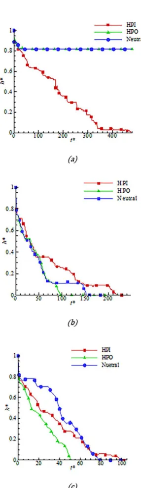
In Fig. 10, the rates of penetration h* versus t* were

shown for three different porosities under three

conditions: (i) hydrophilic, (ii) hydrophobic, and (iii) neutral. As shown in Fig. 10, in high porosities when

solid surfaces were hydrophobic, the rate of fluid

penetration was larger than that of the neutral case. In

the hydrophilic condition, due to the tendency of fluid

to wet the surfaces, it would take more time to separate from the surfaces and penetrate in. By decreasing the porosity, the results obtained were changed.

In the case of a porous medium with hydrophobic

surfaces, the fluid did not completely penetrate inside

the medium. This means that the droplet spread gradually on the top surface of the porous medium. In the hydrophilic condition, the adhesive force

between fluid and solid cells caused the penetration

Figure 8. Pattern of penetration for ε=0.93, for Bo= 0.07, a) 3rd case,

b) 4th case (The sizes of the computational domain and porous area are

160×175 and 160×118, respectively. The Initial height of liquid film is 50 lu. (red line refers to the border of fluid))

of fluid into the pores. The patterns of penetration

for the aforementioned cases are shown in Fig. 11. As shown, in the hydrophilic situation, the generated

fingers surrounded more lattices (more solids) and the observed fingers were thick (i.e., thick-finger-type).

In the hydrophobic case, the droplet penetrated as it contained the minimum number of lattices and the

fluid-run-away was accelerated due to the formation of thin fingers. We named it the thin-finger-type pattern. The fluid in the case of a thin-finger-type pattern

would need less penetration time in comparison with

the thick-finger-type (as shown in Fig. 11(b)). In the case of hydrophobic surfaces, the displaced fluid was not trapped due to the movement of the fingers. The average velocity of the penetrating fluid was also

reported in Table 2. Under the hydrophobic condition,

the calculated penetration velocity of fluid into the

medium (u_hydrophobic=0.0092 lu/s) was 1.77 times faster than that in the hydrophilic condition (u_ hydrophilic=0.0052 lu/s).

Confidence Interval in Different Configurations

Since the porous medium was generated randomly;

there were several different configurations for each porosity value, which would influence the rate and pattern of penetration. Therefore, different configurations of two porosities were considered to investigate the effect of these configurations on the

reliability of results. The rate of penetration in several

configurations is different, so just the average values of penetration rate and offsets from the averaged values

were plotted in Fig. 12. The deviation from the average value (in time steps) was vigorous in low porosity. However, since the general manner of penetration was similar, one can generate various random patterns for the domain to study one individual problem. In general, penetration time would increase 434 percent by decreasing the porosity from 0.9 to 0.8. It would also increase 65.4% when ε = 0.9 and the surface condition changed from hydrophilic to hydrophobic. When the surface condition changed from hydrophilic to hydrophobic while ε = 0.8, the penetration time would increase about 49.3%.

Percent of Hydrophobicity

As shown in Fig. 10 and Fig. 11, when all the solid nodes were hydrophobic, the rate of penetration was much more than in other cases. However sometimes it would cost more to makethe entire medium hydrophobic. In other words, to make a surface hydrophobic, it is necessary to cover the surface with

Figure 10. The rate of penetration h*versus t*, Re=72, Ca=1.1,

Figure 11. Pattern of penetration in two cases for ε=0.8, (a) hydrophilic

situation, (b) hydrophobic situation. (The initial radius of the droplet is set to 20 lu , 80 × 200 computational domain is considered, Re=72, Ca=1.1(red line refers to the border of a drop))

Figure 12. The confidence intervals for (a) hydrophobic, (b) hydrophilic

conditions.

Figure 13. The rate of penetration h* versus t* for different hydrophobicity

for ε=0.8,Re=72,Ca=1.1

special materials similar to the case observed in the

"Gas Diffusion Layer" of PEM Fuel cells. If there

was a way to have the same rate of penetration using cheaper methods, it would have a great impact. Here, we introduce the ‘‘Percent of Hydrophobicity, ƒ" parameter. Using this parameter enables us to produce

layered porous media with different hydrophobicity coefficients. “Percent of Hydrophobicity” could be defined as the number of hydrophobic solid nodes encountered by fluids to the whole number of solid

nodes (the rest of solid nodes were considered hydrophilic) in each layer. Thus, ƒ=1 means that all the solid nodes were hydrophobic; while, ƒ=0.1 means

that 10% of the solid nodes which encountered fluid

in each layer were hydrophobic and the others were hydrophilic. It should be noted that the selection of solid nodes is random.

In Fig. 13, the rate of penetration, h*, versus time,

t*, for different hydrophobicity percentages (when

ε=0.8) is plotted. As shown, the penetration happened by changing the value of ƒ. The rate of penetration was reduced when ƒ is reduced. However, for ε>0.8, the penetration rate was less sensitive to the reduction of” ƒ" and it took less time until the liquid completely penetrates into the medium. It would depend on the

user to choose the hydrophobicity coefficient that satisfies his/her needs the best, instead of using the

costly ideal condition (ƒ=1). Up to this section, all

Figure 14. The rate of penetration h* versus t* for different hydrophobicity

coefficient for ε=0.85, Re=72, Ca=1.1

Here we investigate the effect of heterogeneity of hydrophobicity coefficient in different layers on the

penetration rate and the pattern. The comparison

between different cases was shown in Fig. 14 when

ε=0.85. In this condition, the percent of hydrophobicity

(ƒ) was tuned for each layer which caused a specific

value in each layer. As shown, there was a layout for distribution of ƒ (in the layers) that improved the rate of penetration (see the distribution of ƒ=0.8, 0.6, 0.4, 0.2 for which the average value of ƒ is equal to 0.5 in

the entire medium). Strictly speaking, fluid penetrated

more quickly than the case in which all the layers had the same percent of hydrophobicity (i.e., ƒ= 0.5 in Fig. 14). Using this method, we could increase the

penetration rate for a specified distribution of ƒ and

thus compare the case to the ideal condition (with ƒ=1).

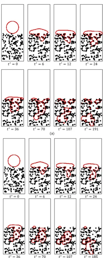
In Fig. 15 penetration patterns for two cases when ε=0.8 are shown. As illustrated in Fig. 15(a) the first

layers were less hydrophobic so they obeyed a piston-type penetration pattern and they wet more nodes. If the layers follow an increasing pattern in their percent of hydrophobicity as they get deeper, the droplet

penetrates like a finger (and it followed a finger-type

penetration regime). If there was an empty space in layers (due to existence of hydrophobic surfaces), a

drop would fill it and would not propagate (as shown

for t* = 36 - 107). Instead, when the first layers were

more hydrophobic, the penetration regime at first was fingering and then it obeyed a piston-type regime

passing through the less hydrophilic layers (Fig. 15(b)).

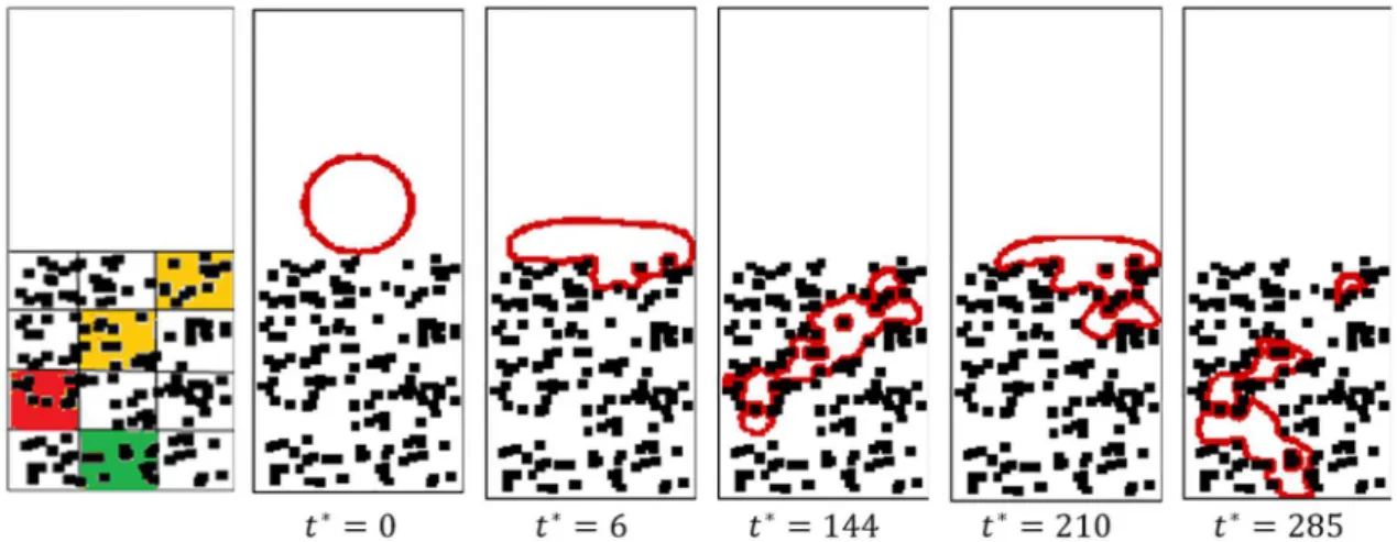
Navigate the Drop into the Porous Medium

Sometimes it is very important to route the fluid

(or droplet) in the porous medium, like in the fuel cell industry, oil exploitation and rain water penetrating

Figure 15. Pattern of penetration in two cases for ε=0.8, (a) f= 0.2,0.4,0.6,0.8

into the ground. To navigate the droplet motion, we

split the domain into several parts with different hydrophobicity coefficient. Here, all parts have ƒ=1 and just some desired parts (color sections) have different

values. In Figs. 16 and 17, the path of motion of liquid in the porous medium was illustrated. The Re and Ca

of the flow were set to 24 and 0.37, respectively. The specified path in Figs. 16 and 17 is related to the yellow, red and green colors which have different

values of ƒ of 0.1, 0.05 and 0, respectively. The arrangement of solid obstacles in the computational domain is random. As the porous medium was more uniform (particularly in the desired direction), navigating the penetration was more predictable. In other words, due to the agglomeration of solid obstacles

in a specific zone and the presence of empty spaces in

the next zones, the penetration may stop in that zone and it would continue in empty spaces. The main goal here was manipulating the droplet penetration in a

specified path.

CONCLUSION

In the current study, the penetration rate and pattern of a two-dimensional droplet has been simulated. The pseudo-potential model was used and a layered porous substrate is generated randomly with square obstacles in which the porosity could be set to the desired values in each layer. A two-dimensional droplet is located tangentially to the substrate surface and injected with initial velocity into the layered porous medium as a result of the gravity force. The regime of penetration

has been studied; capillary fingering and viscous fingering have been observed. The effect of porosity

and hydrophilic/hydrophobic surface on penetration

Figure 16. Specified path and results of simulation for ε=0.8. (The initial radius of the droplet is set to 20 lu , the 80 × 200 computational

domain is considered, Re=24, Ca=0.37(In specified path, yellow, red and green colors show different values of ‘f’ as 0.1, 0.05 and 0

respectively))

Figure 17. Specified path and results of the simulation for ε=0.8, Re=24,

Ca=0.37(In specified path, yellow, red and green colors show different

values of ‘f’ as 0.1, 0.05 and 0 respectively)

rate and penetration pattern was investigated. A new

parameter has been defined as the hydrophobicity coefficient which could be adjusted in different

layers, as required. This parameter could change the penetration pattern. By splitting the layers in some

ACKNOWLEDGMENT

This work has been supported by the Center for

International Scientific Studies & Collaboration

(CISSC).

REFERENCES

Buick, J.M., Greated, C.A., Gravity in a lattice Boltzmann model, Physical Review E, 61(5), 5307 (2000). Dong, B., Yan, Y.Y., Li, W., Song, Y., Lattice Boltzmann

simulation of viscous fingering phenomenon of immiscible fluids displacement in a channel, Computers & Fluids, 39(5) 768-779 (2010).

Dong, B., Yan, Y.Y., Li, W., LBM Simulation of Viscous Fingering Phenomenon in Immiscible Displacement of Two Fluids in Porous Media, Transport in Porous Media, 88(2) 293-314 (2011).

Dullien, F. A. L., Porous media: fluid transport and pore

structure, Academic Press, San Diego (1992).

Gunstensen, A.K., Rothman, D.H., Zaleski, S., Zanetti,

G., Lattice Boltzmann model of immiscible fluids,

Physical Review A, 43(8), 4320 (1991).

Huang, H., Wang, L., Lu, X.-Y., Evaluation of three lattice

Boltzmann models for multiphase flows in porous

media, Computers and Mathematics with Applications, 61(12) 3606-3617 (2011).

Huang, H., Huang, J.-J., Lu, X.-Y., Study of immiscible displacements in porous media using a color-gradient-based multiphase lattice Boltzmann method,

Computers & Fluids, 93 164-172 (2014).

Huang, H., Sukop, M., Lu, X.-Y., Multiphase Lattice Boltzmann Methods: Theory and Application, Wiley, (2015).

Lee, T., Liu, L., Lattice Boltzmann simulations of micron-scale drop impact on dry surfaces, Journal of Computational Physics, 229(20) 8045-8063 (2010). Lenormand, R., Zarcone, C., Sarr, A., Mechanisms of the

displacement of one fluid by another in a network of

capillary ducts, Journal of Fluid Mechanics, 135 337-353 (1983).

Lenormand, R., Touboul, E., Zarcone, C., Numerical models and experiments on immiscible displacements in porous media, Journal of Fluid Mechanics, 189 165-187 (1988).

Liu, H., Valocchi, A., Kang, Q., Werth, C., Pore-Scale Simulations of Gas Displacing Liquid in a Homogeneous Pore Network Using the Lattice Boltzmann Method, Transport in Porous Media, 99(3) 555-580 (2013).

Maghrebi, M.J., Nazari, M., Armaghani, T., Forced

Convection Heat Transfer of Nanofluids in a

Porous Channel, Transport in Porous Media, 93(3) 401-413 (2012).

Nabovati A., Pore Level Simulation of Single and Two Phase Flow in Porous Media using Lattice Boltzmann Method, PhD Thesis, Mechanical Engineering, NEW BRUNSWICK (2009).

Nazari, M., Kayhani, M.H., Mohebbi, R., Heat Transfer Enhancement in a Channel Partially Filled with a Porous Block: Lattice Boltzmann Method, International Journal of Modern Physics C, 24(9), 1350060 (2013).

Nazari, M., Mohebbi, R., Kayhani, M.H., Power-law

fluid flow and heat transfer in a channel with a

built-in porous square cylinder: Lattice Boltzmann simulation, Journal of Non-Newtonian Fluid Mechanics, 204 38-49 (2014).

Nazari, M., Ashouri, M., Kayhani, M.H., Tamayol, A., Experimental study of convective heat transfer of

a nanofluid through a pipe filled with metal foam,

International Journal of Thermal Sciences, 88 33-39 (2015).

Roberts, I.D., Griffiths, R.F., A model for the

evaporation of droplets from sand, J. Atmospheric Environment, 29(11) 1307-1317 (1995).

Salah, Y.B., Tabe, Y., Chikahisa, T., Gas channel optimisation for PEM fuel cell using the lattice Boltzmann method, J. Energy Procedia, 28 125-133 (2012).

Salehi, A., Abbassi, A., Nazari, M., Numerical Solution of Fluid Flow and Conjugate Heat Transfer in an Channel Filled with Fibrous Porous Media-A Lattice Boltzmann Method Approach, Journal of Porous Media, 17(12), 1075 (2014).

Shan, X., Chen, H., Lattice Boltzmann model

for simulating flows with multiple phases and

components, J. Physical Review E, 47(3), 1815 (1993).

Shan, X., Chen, H., Simulation of nonideal gases and liquid-gas phase transitions by the lattice Boltzmann equation, Physical Review E, 49(4), 2941 (1994).

Shan, X., Doolen, G., Multicomponent lattice-Boltzmann model with interparticle interaction, J. Stat. Phys., 81(1-2), 379-393 (1995).

Shan, X., Doolen, G., Diffusion in a multicomponent

Sukop, M.C., Thorne, D.T., Lattice Boltzmann Modeling, 1 ed., Springer-Verlag Berlin Heidelberg, Florida USA (2006).

Swift, M.R., Osborn, W. R., and Yeomans, J.M.,

Lattice Boltzmann simulation of nonideal fluids,

Phys. Rev. Lett., 75(5), 830 (1995).

Taghilou, M., Rahimian, M.H., Investigation of

two-phase flow in porous media using lattice Boltzmann method, Computers & Mathematics

with Applications, 67(2) 424-436 (2014).