1
... .,..FUNDAÇÃO ... GETULIO VARGAS
EPGE
Escola de Pós-Graduação em Economia
~
"The Distribution of Male
Wages
in Brazil"
Prof. N aercio Menezes Filho
(USP)
LOCAL
Fundação Getulio Vargas
Praia de Botafogo, 190 - 100 andar - Auditório
DATA
29/07//99 (58 feira)HORÁRIO 16:00h
•
The Distribution of Male Wages in Brazil:
Some Stylised Facts
Naércio Aquino Menezes-Filho
Reynaldo Fernandes
Paulo Picchetti
Department of Economics Universidade de São Paulo
Abstract
This paper examines the evolution of wage inequality in Brazil in the 1980s and 1990s . It tries to investigate the role played by changing economic returns to education and to experience over this period together with the evolution of within-group inequality. It applies a quantile regression approach on grouped data to the Brazilian case. Results using repeated cross-sections of a Brazilian annual household survey indicate that :
i) Male wage dispersion remained basically constant overall in the 1980's and 1990' s but has increased substantially within education and age groups.
ii) Returns to experience increased significantly over this period, with the rise concentrated on the iliterate/primary school group
iii) Returns to college education have risen over time, whereas return to intermediate and high-school education have fallen
iv) The apparent rise in within-group inequality seems to be the result of a fall in real wages, since the difference in wage leveIs has dec1ined substantially over the period, especially within the high-educated sample.
v) Returns to experience rise with education. vi) Returns to education rise over the life-cycle. vii) Wage inequality increases over the life-cycle.
The next step i~ this research will try to conciliate all these stylised facts.
Acknowledgements: We would like thank Renata deI Pelicio for excellent research
•
•
1 - lntroduction
There has recently been a renewed interest in the role of technological change
in the labour market. This has been spurred by several events. Many comentators have
pointed to a large increase in earnings inequality in Britain and in the V.S. (and to a lesser
extent other European countries), for which technology is frequently seen as the major
culprit.! The argument is that the rapid increase in skilled workers' reI ative remuneration,
accompanied by the rise in education qualifications, drives fundamentally from a demand
shock which would be associated with the computer revolution.
This paper is an attempt to investigate this issue in the Brazilian context. This is
important for several reasons. One ofthe main features ofthe Brazilian economy is its
extremely wide wage and income distribution. A study by Psacharopoulos (1991), for
example, shows that among 56 countries in the world, Brazil is the most unequal. The
proportion of income appropriated by the 10% richest families was about 50% in Brazil in
early 1980s, whereas the 40% poorest got only 7%? Also, Squire and Zou (1998) present
new data on Gini coefficients which has Brazil on the top ofthe list with an average (over
time) coefficient of57.8 reI ative to a sample mean (s.d.) of36.2 (9.2). Moreover, the
important institutional differences between Brazil and most European and North American
countries, especially its extremely high and inflation rates over the 1980s and the high
proportion of employees in the infonnal sector ofthe economy, make a comparison ofthe
Brazilian experience with labour market trends in Europe and V.S. worth investigating.
The leveI and dispersion ofwages in a country at a point in time will in general
depend on the distribution of characteristics ofworkers such as education, effort,
experience, other observed and unobserved skills and on the returns to these
characteristics. These returns will, in turn, depend on the distribution ofthe demand for
these characteristics. Institutional factors like trade unions and minimum wages may also
affect the wage structure. With respect to the evolution ofwage inequality over time, it can
I See Freeman and Katz (1997) for some internacional comparisons and Johnson (1997) for an interesting
explanation.
2 The equivalent numbers for the U.S. were (23% and 17%), for the UK (23% and 18%), Sri lanka (34%
•
•
- - - - .---~---~
be thought to depend on time, experience and cohort effects (see Gosling et aI, 1998). The
time (or macro) effects include changes in economic environrnent, such as institutional
factors, inflation and unemployment rates that affect the workforce as a whole. Increasing
retums to education that affect alI individuaIs at a point in time would enter under this
heading. Experience effects would, for example, reflect an increasing wage dispersion over
the life-cyc1e, together with an aging population. FinalIy, cohort effects reflect permanent
changes in the composition ofthe population due to differences in the characteristics of
new entrants vis-a-vis leavers in the labour market (such as the size ofthe cohort and the
leveI, quality and inequality of schooling). For example, Gosling et aI (1998), using UK
data, find that wage dispersion increased for workers of younger cohorts (conditional on
age and time effects) and that this may reflect an increasing diversification of education.
Moreover, the authors show that returns to education increased for new cohorts and that
wage dispersion tends to increase over the life-cycle, mainly for individuaIs with low leveIs
of education.
There is an extensive literature on the reasons underlying the high leveI of income
inequality in Brazil. The existing explanations range from the country's historical
background to the educational composition ofthe workforce and institutional factors, such
as labour market segmentation and discrimination (see Cacciamali, 1993, for a review). AlI
in alI, it seems inescapable to conc1ude that any reasonable explanation for the income and
wage inequality in Brazil has to be linked to education. Brazil is a country with a high leveI
of education inequality and the retums to education are also very high, as compared to other
countries (see Lam and Levinson, 1992). Barros (1997) for example, estimates that
education explained, ceteris paribus, from 35% to 50% ofwage inequality in Brazil on
average in the 1980s.3
There have also been marked increases in inequality in Brazil since the 1960's.
Bonnelli and Ramos (1995) for instance, show that the Gini coefficient increased from
0.500 in 1960 to 0.568 in 1970, 0.580 in 1980 and 0.615 in 1990. There is much less
agreement on the causes underlying this rapid rise in inequality. In a landmark study,
3 Barros (1997) also estimates that the sector ofactivity is responsible, ceteris paribus, for about 15% of inequality in Brazil, that formal/informal segmentation for about 7%, that regional differences account for 2% to 5%, gender discrirnination for about 5%, racial discrimination for 2%, and that 5% are returns to
•
1-1
I
Langoni (1973) conc1udes that education was responsible for about 58% ofthe increase in
inequality between 1960 and 19704. Some other studies, however, emphasize the role of
institutions like govemment wage policies, weakening oftrade unions, etc. (see Cacciamali,
1993). More recently, some studies have played down the role of education in the
increasing inequality, emphasing instead macroeconomic effects, such as inflation and
gdp-growth.5
The main piece ofBrazilian evidence emphasizing the role of cohort effects is Lam
and Levinson (1992). The authors investigate the re1ationship between the distribution of
years of schooling and income inequality in Brazil and document a significant rise in mean
years of schooling in Brazil for more recent birth cohorts and a fall in the variance. This
fact, together with an increasing residual variance and returns to schooling with age,
means that wage inequality tends to increase with age in Brazil in a point in time.
This paper also intends to focus on the evolution ofwage inequality in Brazil in
1980's. We intend to build upon Lam and Levison (1992) in order to understand the
behaviour of the economic returns to education and to experience over time by relaxing the
assumption that cohorts are perfectly substitutable to each other in the Brazilian economy.
If, for example, technological improvements lead to differential returns to education
between young and older workers, as new entrants into the labour market may be more
vulnerable to changes in demand for labour, then returns to experience will change over
time and this would be interpreted as a cohort effect. This has special significance if there
are changes in the quantity, quality and inequality of education across generations (which,
as we show below, is case in Brazil).
Ther main aim ofthis paper is to investigate the behaviour of the wage
inequality in Brazil in the 1980s and 90s. With repeated cross-sections and an specification
developed by MaCurdy and Mroz (1991) and used by Gosling et aI (1998), it is possible, in
principIe, to disentangle de-trended time effects (constructed as to average zero over the
sample period) from trend and life cyc1e effects, as determinants ofthe evolution ofwage
4 Ofwhich 35% due to compositional changes and 23% to changing economic retums to education .
5 Bonnelli and Ramos (1990) state that education is responsible for about 15% ofthe increase in inequality
•
..
inequality. Therefore, we intend to net out macro-effects and go deep into the structural
causes of tlie rise in inequality in Brazil in the 1980s.
2- Econometric Methodology
As we saw above time, cohort and age effects may seem important in driving
the increase in wage inequality. Unfortunately it is impossible to disentangle their separate
effects, due to a fundamental identification problem. As Heckman and Robb (1985) point
out, birth cohort (c) is completely determined by age (a) and a time trend (t):
c=t-a (1)
We try to model the wage equation in a parsimonious way, following MaCurdy and Mroz(1995) with functions oftime, age and cohorts as follows:
lw
=
a+
A(a)+
T(t)+
C(c)+
R(a,c,t) +u (2)where the functions R are inc1uded to try and capture interactions between age, time and cohorts, like changing returns to experience over time. When exploring third order
interactions between cohort, time and age:
A(a)
=
Ala + A2a2+
A3a3T(t) = J;t
+
T2t2+
1;t
3C(c)
=
Clc + C2C 2+ C3C3
we know that because ofthe identification problem, out ofthe 18 coefficients associated
with third order terms, only 9 linear combinations ofthem can be identified. We therefore,
,
and the estimated parameters are in fact:
A) = (A) -K)),
7;
=
(7;
+
K) ) ,This fact must be kept in mind, when interpreting the results of the regressions. The error
term in (3) inc1ude time effects:
that are constructed to be orthogonal to the age and trend functions, that is, they include no
trends AlI trends in the data will then be reflected in the age and trend variables.
fu the empirical investigation below we wilI break the data into education, year
and age celIs using the fact that our variables of interest are all discrete. We then compute
different sample percentiles ofthe wage distribution and estimate (weighted) linear
regression models on the grouped data for each quantile and education group separately, as
in Chamberlain (1993). Ifall percentiles evolve in the same way (apart form an intercept
shift), then the changing dispersion ofwages can be explained by changing prices andlor
composition of observed skill characteristics. The median defines the location ofthe
distribution and the percentiles around it describe the changes in dispersion.
We therefore have:
The set of functions Tq for each quantile wiIl measure differences in wages over time. The
difference in these functions between the top and bottom of the distribution will capture
trend effects on the within-groups dispersion of wages. The difference across education
---~---~~-~----~
~
,
•
functions Aq measure how the wage distribution changes as each education group gets
older. The changes in the median will reflect experience effects and differential rates of
leaming by doing will mean that the variance ofwages will increase with age (see Mincer,
1974 and Farber and Gibbons, 1997). Common shocks to the wage distribution UI are the
same for each educational group regardless of age, such as macroeconomic effects common
to all individuaIs at any point in time.
We proceed as follows: We first choose within each cell a population characteristic of
interest and estimate it using the corresponding sample characteristic. We estimate the
median, 10th, 25th, 75th and 90th percentiles for each age, year and education cell. This
equivalent to using the fulI sample to regress wages on all education year and age
interactions. The percentiles are asymptotically nonnally distributed (see Koenker and
Portnoy, 1998). The variance ofthese estimated order statistics is given by
V(q)=q(1-q) (6)
f(q)2
We estimate f( q) (conditional density) using a Gaussian Kernel with bandwith equal to half
the standard deviation ofwages for each cell.
We then try to impose some structure on the wage distribution by means of a
minimum distance estimator. The minimum distance procedure chooses
f3
such as tomlmmlse:
(q - pzrV(qrl (q -
PZ)
(7)where q are the estimated order statistic and Z is a set of linear restrictions.
Under the null that the restrictions are valid, the minimised value follows a chi-squared
distribution with degrees of freedom equal to the number of restrictions. As this is like
weighted Ieast squares, the grouped regression procedure wilI give us consistent estimates
and alI we have to do to construct the test statistic is to sum the weighted squared residuaIs,
i.e. the empiricaI percentiles minus the age and trend effects, minus the orthogonal time
- - - - . - - - -
---~---~:
•
3 - Data
fu this paper we use a particularl y rich data set, consisting of repeated
cross-sections of an annual household survey, conducted every September by the Brazilian
Census Bureau. It consists of around 125,000 annual individual levei data. From the original data we kept only male (to avoid the usual composition problems due to changes
in female participation), with positive hours worked in the reference week, positive
monetary remuneration, with between 25 and 55 years of age. The final sample have
706,782 observations in the low education group (O to 4 years ofschooling) 214,077 in the
intermediate one (5 to 8), 161,355 in the (some) high school group and 110,883 in the
(some) college one. The sample period ranges from 1977 to 1996.
The main variable used in this analysis is real hourly wage, defined as normallabour
income in the mainjob in the reference month normalised by normal week1y working
hours. The nominal wage was deflated using the Brazilian consume price index (IPCA) and
took into account the change in currency that took place in 1986.
4 - Results
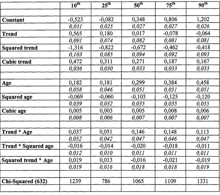
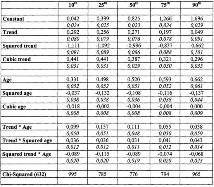
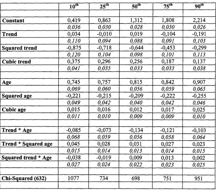
Tables 1 to 4 present the main results ofthe paper. Although the results are best
interpreted in terms of the figures presented in the end of the paper, some points deserve
mentioning. Firstly, all coefficients seem to have been precisely estimated. Secondly, there
are important differences both among the different percentiles within each education group
and across different education groups. Thirdly, the coefficients on the interactions between
trend and age tend to be significant in all education groups and percentiles, which means
that returns to experience are seem to be changing in the sample period. Finally, the
Chi-squared test tends to reject the restrictions in alI specifications, which raises serious doubts
about the explaining power ofthe restricted model.
The examination ofthe figures tell a very interesting story. Figures 1 and 2 plot the
predicted median wages for the first and fourth education group respectively, for different
..
•
..
sample period. It is also interesting to note that real wages have fallen dramaticalIy over time for alI·education groups. Figures 3 and 4 do the same for the 90th percentile and the
results are similar though the fit is a not quite as good. Figures 5 and 6 show that, although
we are able to folIow the evolution ofthe 90/1 O differential of (log) wages quite c10sely for
the lowest education group, the results are poor if one consider the college group, especially
at higher ages. This is probably the result of the small sample size in these cells.
Graph 7 plots the evolution of the trend effect on wages (abstracted from cyc1ical
effects), for those with 44 years of age. It seems c1ear that real wages have falIen for alI groups, but the falI was markedly lower for the highest eudcation group. This resulted, as
shown in figure 8, in a rise in the retums to college education in Brazil, together with a falI
in the returns to intennediate and high school education. This has taken place across the
wage distribution, as shown by figures 9 and 10.
On the evolution ofthe wage inequality over time, figures 11 and 12 show that the
90/1 O ratio of smoothed predicted wages has increased in Brazil over the sample period
withing education groups, apart from the intennediate education group. To check whether
this rise in inequality is the result of a rise in the spread or a fall in the median, figures 13
and 14 plot the predicted wages from a regression ofthe leveI ofwages on age and trend.
The results are impressive, as it seems that the absolute leveI of inequality has decreased for
the higher education groups and remained roughly constant for the less educated.
Tuming now to the age effects, Figure 15 shows that there are important interactions
between education and experience, as evidenced by the significant differences in the age
pro files across education goups. Retums to experience are higher for the more educated.
This is also reflected in figure 16, which shows that the retums to education tend to
increase over the life cyc1e. The results ofthe interactions between age and trend are plotted
in figures 17 to 20. It seems that retums to experience have risen mostly for the low education group, whilst have risen from 1977 to 1987 and then fallen in 1996 for the other
groups.
Figures 21 to 24 show that the retums to experience vary dramatically across
percentiles, especially for the low education groups. Significantly, for the high education
groups, there is almost no variation. Finally, figure 25 shows that inequality tends to
•
•
JV
These results are evidence that the wage behaviour over the life cyc1e in Brazil is similar to
the UK, nofwithstanding the differences between the two countries in various aspects.
4 - Conclusions
•
5 - References
Baker, G., Gibbs, M. and Holmstrom, B. (1994) - "The Wage Policy ofthe Firm", QuarterlyJournal ofEconomics, 109,921-955.
22/97.
Barros, R. (1997) - "Os Determinantes da Desigualdade no Brasil", USP-DP
Bonelli, R. and Ramos, L. (1995) - "Distribuicao de Renda no Brasil", Revista Brasileira de Economia, 49,353-373.
Cacciamalli, M. C. (1997). - "The Growing Inequality inIncome Distribution in Brazil" in Willumsen and Fonseca (eds) - Brazilian Economy: Structure and Performance in Recent Decades, North-South Center Press.
Freeman, R. and Katz, L. (1997). Changes and Differences in Wage Structures.
Chicago IL, University of Chicago Press.
Gosling, A., Machin, S. and Meghir, C. (1998) - "The Changing Distribution of Male Wages in the UK", Centre for Economic Performance Discussion Paper 271.
Johnson, G. (1997) - "Changes in Earnings Inequality: The Role ofDemand".
Journal ofEconomic Perspectives, 11,41-54.
33-50. Koenker, R. and Basset, G. (1978) - "Regression Percentiles", Econometrica, 46,
Lam, D. and Levinson, D. (1992).- Declining Inequality ofSchooling in Brazil and its Effect on Inequality ofWages" ,Journal ofDevelopment Economics, 37, 199-225.
Langoni, G. (1973) -Distribuicao de Renda e Cerscimento Economico.
Expressa0 e Cultura.
MaCurdy, T. and Mroz (1991) - "Estimating Macro Effects from Repeated Cross-Sections", University of Standford, mimeo.
Psacharopoulos, G. (1991) - "Time Trends ofthe Returns to Education: Cross-National Evidence", Economics and Education Review, 8, 3.
-IC
Table 1 - Education between O and 4 years of schooling
10th 25th 50th 75th 90th
Constant -0,523 -0,082 0,348 0,806 1,202
0,031 0,025 0,027 0,027 0,026
Trend 0,565 0,180 0,017 -0,078 -0,064
0,091 0,074 0,082 0,081 0,081
Sguared trend -1,316 -0,822 -0,672 -0,462 -0,418
0,103 0,085 0,094 0,092 0,093
Cubic trend 0,472 0,311 0,271 0,187 0,167
0,036 0,030 0,033 0,033 0,033
A~e 0,182 0,181 0,299 0,384 0,458
0,058 0,046 0,051 0,051 0,051
Squared a2e -0,069 -0,060 -0,103 -0,125 -0,120
0,039 0,032 0,035 0,035 0,035
Cubic age 0,005 0,003 0,005 0,008 0,006
0,008 0,006 0,007 0,007 0,007
Trend
*
Age 0,037 0,051 0,146 0,148 0,1130,052 0,042 0,047 0,046 0,047
Trend
*
Squared age -0,016 -0,014 -0,020 -0,018 -0,0110,012 0,010 0,011 0,011 0,011
Sguared trend
*
Age 0,019 0,013 -0,016 -0,021 -0,0190,019 0,016 0,018 0,018 0,019
Chi-Squared (632) 1239 786 1065 1109 1331
Table 2 - Education between 5 and 8 years of schooling
10th 25th 50th 75th 90th
Constant 0,042 0,399 0,825 1,266 1,696
0,024 0,025 0,023 0,024 0,029
Trend 0,292 0,256 0,271 0,197 0,049
0,080 0,079 0,076 0,078 0,091
Squared trend -1,111 -1,092 -0,996 -0,837 -0,662
0,091 0,089 0,086 0,088 0,101
Cubic trend 0,441 0,441 0,387 0,321 0,296
0,031 0,031 0,029 0,030 0,035
Age 0,331 0,498 0,520 0,593 0,662
0,052 0,052 0,051 0,052 0,061
Squared age -0,037 -0,132 -0,108 -0,116 -0,137
0,038 0,038 0,036 0,038 0,044
Cubic age -0,018 -0,002 -0,004 -0,004 0,000
0,008 0,008 0,008 0,008 0,009
Trend
*
Age 0,099 0,157 0,111 0,055 0,0380,050 0,051 0,048 0,050 0,059
Trend
*
Squared age 0,036 0,036 0,031 0,041 0,0430,012 0,012 0,011 0,012 0,014
Squared trend
*
A~e -0,089 -0,115 -0,089 -0,074 -0,0680,020 0,020 0,019 0,020 0,023
Chi-Squared (632) 995 785 776 794 965
Table 3 - Education between 9 and 11 years of schooling
10th 25th 50th 75th 90th
Constant 0,419 0,863 1,312 1,808 2,214
0,036 0,030 0,028 0,030 0,026
Trend 0,034 -0,010 0,019 -0,104 -0,191
0,110 0,094 0,088 0,091 0,103
Squared trend -0,875 -0,718 -0,644 -0,453 -0,299
0,120 0,104 0,098 0,101 0,113
Cubic trend 0,375 0,296 0,256 0,187 0,137
0,041 0,035 0,033 0,033 0,038
Age 0,745 0,757 0,815 0,842 0,907
0,069 0,060 0,056 0,059 0,065
Squared a2e -0,221 -0,215 -0,209 -0,222 -0,255
0,049 0,042 0,040 0,042 0,046
Cubic age 0,015 0,016 0,012 0,017 0,025
0,011 0,010 0,009 0,009 0,010
Trend
*
Age -0,085 -0,073 -0,134 -0,121 -0,1030,068 0,059 0,056 0,058 0,064
Trend
*
Squared age 0,045 0,028 0,031 0,027 0,0230,015 0,014 0,013 0,014 0,015
Squared trend
*
Age -0,038 -0,019 0,009 0,013 0,0020,027 0,024 0,022 0,023 0,025
· Table 4 - Education more than 12 years of schooling
10th 25th 50th 75th 90th
Constant 0,937 1,393 1,961 2,515 2,902
0,041 0,030 0,035 0,034 0,036
Trend -0,011 -0,046 -0,243 -0,561 -0,805
0,124 0,113 0,100 0,097 0,103
Squared trend -0,657 -0,553 -0,354 -0,071 0,393
0,141 0,125 0,111 0,108 0,114
Cubic trend 0,288 0,234 0,174 0,027 -0,066
0,049 0,043 0,039 0,038 0,040
A2e 1,106 1,216 1,215 1,106 1,157
0,080 0,060 0,067 0,066 0,069
Squared age -0,446 -0,500 -0,510 -0,448 -0,498
0,056 0,050 0,045 0,045 0,047
Cubic age 0,054 0,065 0,068 0,059 0,071
0,012 0,011 0,010 0,009 0,010
Trend
*
Age -0,048 -0,071 -0,039 -0,008 0,0080,076 0,068 0,062 0,061 0,065
Trend
*
Squared a2e 0,052 0,040 0,037 0,029 0,0320,018 0,016 0,015 0,014 0,016
Squared trend
*
A2e -0,052 -0,017 -0,020 -0,015 -0,0270,030 0,027 0,024 0,023 0,025
o Iwhm1a + Iwhm1b
o (p 50) Iw
id==24 id==34
.5
o
-.5
id==44 id==54
.5
o
-.5
1975 1980 1985 1990 1995 1975 1980 1985 1990 1995
year
Graphs by id
-\2)
o Iwhm4a
<> (p 50) Iw
+ Iwhm4b
id==24 id==34
3
2.5
2
1.5
..
id==44 id==543
2.5
2
1.5
1975 1980 1985 1990 1995 1975 1980 1985 1990 1995
year
, - - -
~--o Iwh901a + Iwh901 b
o (p 90) Iw
id==24 id==34
2
1.5
.5
id==44 id==54
2
1.5
.5
1975 1980 1985 1990 1995 1975 1980 1985 1990 1995
year
~---~_.~---o Iwh904a + Iwh904b
o (p 90) Iw
id==24 id==34
4
3
2
id==44 id==54
4
3
2
1975 1980 1985 1990 1995 1975 1980 1985 1990 1995
year
o c90101 + p9010
id==24 id==34
2.5'
2
1,5
id="'44 id="'54
2.5
2
1.5
1975 1980 1985 1990 1995 1975 1980 1985 1990 1995
year
@
o c90104 + p9010
id==24 id==34
2.5
2
1.5
id==44 id==54
•
2.5
2
1.5
1975 1980 1985 1990 1995 1975 1980 1985 1990 1995
year
3
2
1
o
o tlw1d
O tlw3d
1975 1980
t:. tlw2d
tlw4d
1985 year
wages over time:age44
1.5
1
.5
o
o tlw21d
O tlw43d
1975 1980
te. tlw32d
1985 1990
year
returns to educ over time:age44
o tlw2110 D. tlw3210
o tlw431O
1
.8
.6
.4
1975 1980 1985 1990 1995
year
o tlw2190 t:. tlw3290
o tlw4390
.9
.8
.7
.6
.5
1975 1980 1985 1990 1995
year
o tlw90101
o tlw90103
1975
•
1980
®
t:. tlw90102
tlw90104
1985 year
90/10 over time:age34
o tlw90101
o tlw90103
2.2
2
1.8
1975 1980
@
6 tlw90102
tlw90104
1985 year
90/10 over time:age44
~O
30
20
10
o
o tw90101
O tw90103
~tw90102
tw90104
:
:
:
:
: :
:
:
:
.& .& .&O O o o O
1975 1980 1985 1990
year
90/10 (Iev) over time:age34
.40
30
20
o tw90101
O tw90103
t::.tw90102
o ilw961
o ilw963
. 3
2
1
o
20
{:, ilw962 ilw964
30 40
idade
returns to exp: 1996
o ilw2196 t:. ilw3296
o ilw4396
1
.8
.6
.4
20 30 40 50 60
idade
@
o nilw771 /:,. nilw871
o nilw961
. 1
.8
.6
.4
.2
20 ~ 40 00 60
idade
@
o nilw772 t; nilw872
o nilw962
1.6
1.4
1.2
1
.8
20 30 40 50 60
idade
o nilw773 !;, nilw873
o nilw963
3
2.5
2
1.5
1
20 30 40 50 60
idade
o ni/w774 I:; nilw874
o nilw964
3
2.5
2
20 30 40 50 60
idade
---~----
---~~---o nilw1 b, ni901
o ni101
.6
.4
.2
o
20 30 40 50 60
idade
o ni/w2 l::. ni902
o ni102
. 1
.5
•
o
20 30 40 50 60
idade
o nilw3 t:. ni903 o ni103
. 1
.5
o
30 40 50 60
idade
o nilw4 t:. ni904 o ni104
1. .5
1
.5
o
20 30 40 50 60
idade
returns to exp: educa4
.6
.4
..
.2
o
•
•
o i90101
o i90103
20
6 i90102 i90104
30 40 50
idade
inequality over the life-cycle
60
-,
.
..
..
000089068
FUNDAÇÃO GETULIO VARGAS
BIBLIOTECA
ESTE VOLUME DEVE SER DEVOLVIDO A BIBLIOTECA NA ÚLTIMA DATA MARCADA
N.Cham. P/EPGE SPE M536d
Autor: Menezes Filho, Naércio Aquino.
Título: The distribution of male wages in Brazil.
089068
1111111111111111111111111111111111111111 52057