Geographic Routing Using Logical Levels in
Wireless Sensor Networks for Sensor Mobility
Yassine SABRI
NTICLaboratory,
HigherInstitute ofApplied Engineering(IGA), El JadidaMOROCCO
Najib EL KAMOUN
STICLaboratory, ChouaibDoukkaliUniversity,
El JadidaMOROCCO
Abstract—In this paper we propose an improvement to the GRPW algorithm for wireless sensor networks called GRPW-M , which collects data in a wireless sensor network (WSN) using a mobile nodes. Performance of GRPW algorithm algorithm depends heavily on the immobile sensor nodes . This prediction can be hard to do. For that reason, we propose a modified algorithm that is able to adapt to the current situation in the network in which the sensor node considered mobile. The goal of the proposed algorithm is to decrease the reconstruction cost and increase the data delivery ratio. In comparing the GRPW-M protocol with GRPW protocol in simulation, this paper demonstrates that adjustment process executed by GRPW-M does in fact decrease the reconstruction cost and increase the data delivery ratio . Simulations were performed on GRPW as well as on the proposed Routing algorithm. The efficiency factors that were evaluated was total number of transmissions in the network and total delivery rate. And in general the proposed Routing algorithm may perform reasonable well for a large number network setups.
Keywords—WSN ; Routing ; Ad hoc ; Localization ; Scalability
I. INTRODUCTION
Remarkable advances have been made in micro-electronicsmechanical system (MEMS) and wireless communication technologies. This development has enabled sensors to collect contexts from the real world. Many sensor nodes compose a wireless sensor network (WSN) that detects data regarding a physiological change or the presence of various chemical or biological materials. An external device, called a base station or a sink, such as a mobile device or a mobile robot, is used to detect events and collect data from the sensing environment. One or multiple mobile sinks move throughout the WSN to gather data coming from all nodes. There is a lot of research on the moving strategy of mobile sinks [1], [2], [3], [4] . Almost all of them use the routing based on the physical locations of nodes for data transmission . It is important to choose a routing protocol for WSN with a mobile sink, because the efficient routing paths between the sensor node and the sink change with time. The greedy forwarding is a candidate because it is simple and efficient about data transmission in WSN. In greedy forwarding, each node just needs to know three pieces of information: its location, the location of neighbors, and the location of the sink. In the WSN with mobile sink, the first two pieces
are fixed and the location of the sink could be broadcasted to the nodes with a virtual backbone [9]. However, greedy forwarding may lead into a dead end when there is no neighbor closer to the destination, and recovery strategy such as GPSR [10] is necessary to guaranty data packets can be delivered to the destination.
Research in WSN has developed fast during the last couple of years and has made the implementation of WSN feasible. However the cost and the size of the nodes in the networks have to be lowered to make the WSN attractive to be used in mainstream applications.
Wireless Sensor Networks (WSN) are constituted of a large number of tiny sensor nodes randomly distributed over a geographical region whose power consumption is low. How-ever, as shown in current research [5] , the classical rout-ing protocols are not applicable to sensor networks in a real environment,mainly because of specific radio conditions. Noise, interference, collisions and the volatility of the node neighborhood leading to a significant drop in performance. Many applications for sensor networks such as monitoring of forest fires, the remote meter reading,...For these cases,The Ge-ographic routing of data in this type of network is an important challenge, Geographic routing uses nodes locations as their addresses, and forwards packets (when possible) in a greedy manner towards the destination. Since location information is often available to all nodes in a sensor network (if not directly, then through a network localization algorithm) in order to pro-vide location-stamped data or satisfy location-based queries, geographic routing techniques are often a natural choice.
II. RELATED WORK AND BACKGROUND
Various routing protocols have been proposed for the WSNs with mobile sinks. In [12], Nazir proposes the Mobile Sink based Routing Protocol (MSRP) in which the sink movement strategy depend on the residual energy information from the cluster-heads and takes the movement based on the residual energy of the cluster-heads [12]. In the Local Update-based Routing Protocol (LURP) [13], a broadcast protocol is proposed to resolve the problem that frequent location updates from the sink can lead to both rapid energy consumption of the sensor nodes and increased collisions in wireless transmissions . The most widely known proposal is [6][7], but several other geographic routing schemes have been proposed [8] One of the key challenges in geographic routing
is how to deal with dead-ends, where greedy routing fails because a node has no neighbor closer to the destination; a variety of methods (such as perimeter routing in GPSR/GFG) have been proposed for this. More recently, GOAFR [9] proposes a method for routing approximately the voids that is some asymptotically worst case optimal as well as average case efficient. Geographic routing is scalable, as nodes exclusively maintain state for their neighbors, and supports a full general any-to-any communication pattern without explicit route establishment. However, geographic routing requires that nodes know their location. While this is a natural assumption in some settings (e.g., sensornet nodes with GPS devices), there are many circumstances where such position information isn’t available.are most often require information about the position of their voisins to function effectively.Or, this assumption is far from the reality.The other, the localization of protocols, used as a preliminary step by geographical routing protocol are not necessarily precise. For example, in [10],the authors proposed localization methods with which sensors determine their positions with a rate of less than about90% positioning in large scale. or, if a node that does not know its location, the node risk of never communicate with other node of networks,and no information will be transmitted to the user and the base station never knows that node.
A lot of work has previously been done on routing protocols for WSN. Most of these protocols have been designed for a specific kind of WSN and have parameters which must be estimated in order to make the system perform effectively.
Mobility of nodes in the network adds a significant challenge. The study of routing over mobile ad hoc networks (MANET) has indeed been an entire field in itself, with many protocols such as DSR, AODV, ZRP, ABR, TORA [11], [12], etc. proposed to provide robustness in the face of changing topologies [13], [14], [15], [16]. A thorough treatment of networking between arbitrary end-to-end hosts in the case where all nodes are mobile is beyond the scope of this text. However, even in predominantly static sensor networks, it is possible to have a few mobile nodes. One scenario in particular that has received attention, is that of mobile sinks. In a sensor network with a mobile sink (e.g. controlled robots or humans/vehicles with gateway devices), the data must be routed from the static sensor sources to the moving entity, which may not necessarily have a predictable/deterministic trajectory. A key advantage of incorporating mobile sinks into the design of a sensor network is that it may enable the gathering of timely information from remote deployments, and may also potentially improve energy efficiency.
In this paper we propose an enhancement to the GRPW algorithm based on scheduling techniques that allow the sink node to send its position in a planned manner . We propose mobile sensors with limit path in the edge of site which sensor nodes are scattered there. With this manner we dont have security problems of mobile nodes.
When sensor Sink are mobile, it is not reasonable that sink sensor send its position continually, due to constraint of energy. A first work in [7] proposes three methods SFR (Static Fixed Rate), DVM (Dynamic Velocity Monotonic), MADRD
(Mo-bility Aware Dead Reckoning Driven) to determinate periods where a node the sink sensor send its position according to its speed mobility and its previous position. The following sub-sections explain these three methods.
1) Static Fixed Rate (SFR): In this method, the sensor sink send its localization with a fixed time period tsf r .Lets be a
sink sensor. If s sends its localization at timet it obtains its position(xt, yt). In fact,sconsiders that its position is(xt, yt)
during period between tandt+tsf r . This method does not
take into account mobility of the sink sensor. Specifically, if a sink is moving quickly, the error will be high; if it is moving slowly, the error will be low.
2) Dynamic Velocity Monotonic (DVM): In DVM, sensor sink adapts the sending of its position as a function of its mobility: the higher the observed velocity, the faster the node should be localized to maintain the same level of error. Thus when a sink positions it computes its velocity by dividing the distance it has moved since the last localization point by the time that elapsed since the localization. Thus, the node can schedule the next localization point at the time when a specified distance will be covered if the node continues with the same velocity. Therefore, localization will be carried out more often as soon as the node is moving fast. Conversely, localization will be carried out less frequently as soon as the node is moving slowly. Similar to SFR, the location referred by the node between two localization points will be one calculated at the previous localization point.
3) Mobility Aware Dead Reckoning Driven (MADRD): MADRD is a predictive protocol that computes the mobility pattern of the sensor and uses it to predict future mobil- ity. If the expected difference between the actual mobility and the predicted mobility reaches the error threshold, then localization should be triggered. This differs from DVM where localization must be carried out when the distance from the last localization point is predicted to exceed the error threshold. Therefore, localization can be carried out at very low frequency, if the node is moving predictably. Otherwise, localization will be carried out more often. In the case where the prediction is perfect, node does not carried out localization. However, the predicted mobility pattern will generally be imperfect. Sensors will typically not follow a predictable model; for example, there may be unpredictable changes of directions or pauses that will cause the predicted model to go wrong. For all these reasons it is necessary to continue localization periodically to detect deviations from the predicted model. In this paper contrary to the previous solutions, we consider the case where all sensors are mobile. We propose a new method to locate sensors and to adapt periodicity to invoke the localization procedure in order to obtain high accuracy while reducing energy consumption. We analyze our solutions and compare them to the previous ones and we adapt them in order to take into account positioning error.
A. Motivation
In this paper we select the GRPW algorithm (Geographic Routing Protocol Washbasin). as basis for an investigation on improving the deployment of a network. GRPW is a geograph-ical routing protocol for Wireless Sensor Networks (WSN) ensures a load balancing, minimizing energy consumption and
the rate of message delivery for very low power networks and uses a routing policy with logical levels, inspired from the water flow in a washbasin .
GRPW requires knowledge the immobile sink position which is considered as parameter for initialization of the network to construct the logical levels topology . By changing these parameter a trade off is made between an overhead in the number of transmissions used to setup routing infor-mation in the network and an overhead in the number of transmissions used for sending the queries. In order to set these parameter, the immobile sink node position has to be known before deployment. If GRPW is initialized with mobile sink parameter then it will not be efficient and can in some cases be outperformed by a simple protocol such as classic flooding. In many cases the number of events or queries cannot be expected to be known in advance. As a consequence, GRPW will not always be an attractive routing protocol.
B. Organization
We have organized this paper in the following way: Section II describes the previous work. In this section we will focus on GRPW which is the basis for our extension. In Section III we describe our algorithm and the implementation of it. Section IV describes the simulation details of our algorithm and the results obtained are presented in Section V. In Section VI results are discussed and conclusions presented.
III. GRPWALGORITHM
Several papers have been published about routing in WSN. In this section we will focus on introducing the GRPW Routing approach as this is the foundation for our work. For a more elaborate description to GRPW please refer to [17].
GRPW that each node can get its own location information either by GPS or other location services [18][19]. Each node can get its one-hop neighbor list and their locations by beacon messages. We consider the topologies where the wireless sensor nodes are roughly in a plane.
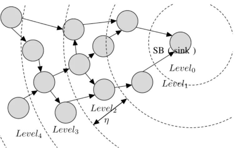
Our approach involves three steps:
Level0
Level1
Level2
Level3 Level4
SB ( sink )
η
Fig. 1: Illustration of GRPW routing network levels
1) The distribution the immobile sink position to all sensors networks: In the first step,The communica-tions in this step are made in three steps:
• When a node wants to transmit the sink position to its neighbors ,it first emits ADV message containing the location of sink.
• A node receiving a message ADV. If inter-ested by this information, it sends a message REQ to its neighbor.
• In Receiving a message REQ, the transmitter transmitted to the node concerned the sink position in a DATA message.
2) Construction of logical levels:In this step the node networks determine its level of belonging through the sink node position,each node u well localized, calculate its level based on the received position of sink in the Phase 1 ,with which u calculates the distance duSink which separates him with the sink
node .the levels is calculated so that the width level
η be constant is less than and inversely proportional to the density of networksδ.
The levell of the node udefined by:
Levelu={l∈N/ duSink
η ≤l≤ duSink
η + 1}
Set of the neighbor nodes that are well localized and which belongs to the same level asu:
LNΛ(u)={v∈NΛ(u)/Levelu=Levelv}
Set of the neighbor nodes that are well localized and which belongs to the higher level thanu:
L+N
Λ(u)={v∈NΛ(u)/Levelu=Levelv−1}
Set of the neighbor nodes that are well localized and which belongs to the lower level thanu:
L−
NΛ(u)={v∈NΛ(u)/Levelu−1 =Levelv}
3) Data forwarding : The routing decision is done in our approach in three modes, depending on dispoini-bilites neighboring nodes and of their level of belong-ing: theEven Forwarding,Anterior Forwardingand theRear Forwarding (respectively called EF, AF and RF).
In the first mode AF ,GRPW constructs a route traversing the nodes of the source to the destination which each node receiving a packet DataPacket with the mode of transport ANTERIOR_FORWORD, will
move toward the intermediate node in its coverage area what in before , the intermediate node select among the neighboring node using a lookup function. Lookup function is used by a node in order that he can determine the next hop to reach the next level, to determine the next hop function, lookup based on the principle of Round Robin (RR). In the second mode EF, on account of the frequent failures of nodes, the mobility of nodes or policy scheduling
of activities used, disconnections can occur in the network generates, so, what are called holes in this situation, GRPW will change the routing mode to
EVEN_FORWORD to reroute the packet in EF mode
and to overcome the void case. In the third mode RF, GRPW reroute the packet DataPacket, who was failed in AF and EF, RF fact sends a packet to the low level
L−
NΛ() by seeking the next hop among neighboring
based on the lookup function. RF is leaning on same technique used in EF, for avoids the routing loop we safeguard the sets of node traversed by the packet DataPacket in a vector-type structure
IV. GRPW-M: ADAPTIVEROUTING FORSENSOR
MOBILITY INWSNS
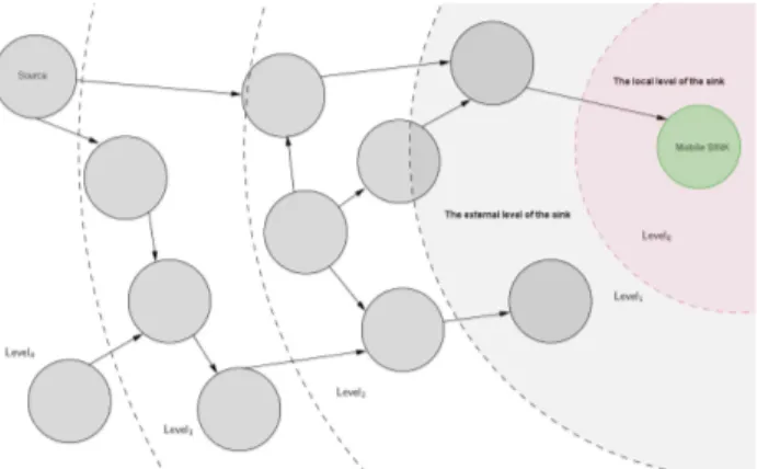
Let us now consider the use of GRPW in a sensor network with static nodes and a single mobile sink. If the sink moves, its virtual level will change, and the messages routed to the old coordinates will not reach the sink. A simple solution would be to notify all the nodes about the sinks new coordinates. This solution, however is expensive in terms of the number of messages, and the corresponding energy consumption.
The GRPW-M algorithm takes an idea which had been successfully applied to geographical routing to reduce the number of update messages necessary to maintain routability. The general idea is that as long as the sink moves inside a limited local level area, the nodes outside that level area will not be notified about the sinks movement. The routing will rely on the nodes at the periphery of the level area to forward the messages to the sink. Thus, the local area will be defined as all the nodes which are belong to the same level to the initial location of the sink :
Note, however, that the current location of the mobile sink might be different . Defining the local level area, we say that the sink can make two different types of moves:
• a local move keeps the sink inside the local level area. In this case, the sink will update only the nodes inside the local level about its new location using one of the scheduling methods previously presented SFR,MADRD or DVM, and the local level area will not change.
• in an external move the sink leaves the current local level area . As a result, the sink must create a new local level area (see Figure 1) and (b) notify the whole network about its new virtual coordinates and new local level area .
GRPW-M uses three type of messages: (a)LOCALmessages carry updates about the local moves of the sink and they are broadcasted only within the confines of the local level area , (b) EXTERNAL messages carry updates about the external move of the sink and they are broadcasted to the whole area and (c)SENSINGmessages which carry data collected by the network, and are transmitted by hop-by-hop transmission from the nodes to the sink (whichever its current location it may be)
Fig. 2: Illustration of GRPW-M routing network
V. SIMULATION
In this section, details about how the simulations were carried out are presented. Using a simulator J-Sim based on the Java programming language, which is able to simulate GRPW-M routing as well as the original routing GRPW .
A. Simulation Specifics
In this section, the simulation results using J-Sim. The sensor nodes were randomly deployed in a monitoring area of 300m×300m, where one node is the mobile sink and the others are static sensor nodes. The number of nodes varied from150 to400 nodes. All sensor nodes had the same communication range and energy, where the communication range was15m.
• The nodes are arranged within a rectangular grid, with every node residing in a particular sector of the grid. As a result, the neighbours of a particular node are determined by the square formed around that node instead of the radial distance computed in the original paper. This, however, should not effect the performance of the algorithm.
• The nodes are placed randomly on the grid, rather than fixing them. As a result, the events are also assigned randomly to the generated nodes.
• The node from which the queries originates is also randomly selected. It is checked that the querying node is not a node which has been assigned the same event as in the query.
• In the simulation , the network lifetime is defined as the time when the first sensor node dies .
In order to ensure reproducibility, all random values are initialized with a seed from the configuration file. This way, any simulation which is run from a particular configuration will generate the same result.
B. Simulation Results
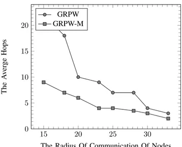
1) Varying the communication radius of nodes: Figs. 3 show the average hops decrease when the communication radius increases. This is caused by the increase of R results the increase of average distance of one hop and fewer nodes
15 20 25 30 0
5 10 15 20
The Radius Of Communication Of Nodes
The
A
v
er
ge
Hops
GRPW GRPW-M
Fig. 3: The average hops whenR is changed.
are required to transmit a packet to the sink. In GRPW, there is a dramatic decrease when R is changed from 15 units to 18 units. This is because the greedy forwarding often fails when the network is a sparse network. Form those result, we can get that GRPW-M outperforms other algorithms when the network is sparse.
100 120 140 160 180 200 220 240 5
10 15 20 25
The Number Of Nodes
The
A
v
er
ge
Hops
GRPW GRPW-M
Fig. 4: The average hops when N is changed.
2) Varying the number of nodes: In Fig. 4, we study the impact of the increasing number of nodes when nodes communication radius is 15 units, the threshold of degree is 5 and the number of nodes increases from 100 to 180. We still assume that there is no failed node in the network. In Figs. 13 and 14, the average hops showing a decreasing trend in generally. The increase of N makes the network denser, therefore, the rout more like to get a shorter path. However, there are some fluctuations because the corresponding param-eters of algorithms influence the virtual coordinates given to nodes. We can get that there is a dramatic decrease about the average hops of GRPW when N increase. This is caused by the
fewer occurrences of hole [10], which result in more nodes are required to transmit the data packet to the sink. Five criteria were adopted to judge the performance and overhead of the different protocols: data delivery ratio, maintenance cost, total packet cost, latency, and hop count. The data delivery ratio was calculated by dividing the number of received packets from the mobile sink by the total number of data packets. A high data delivery ratio demonstrated that the routing protocol could construct and adjust tree routing and deliver data to the mobile sink.
0 5 10 15
1,000 1,500 2,000 2,500
Speed of Mobile Sensorm×sec−1
Number
of
Control
P
ack
ets
GRPW GRPW-M
Fig. 5: The maintenance cost of GRPW-M structures.
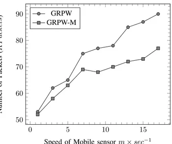
3) The maintenance cost : The maintenance cost repre-sented the total number of control packets, including construc-tion and adjustment packets. A low maintenance cost meant that the routing protocol saved more energy and communi-cation cost, and decreased collisions. The total packet cost included the number of data packets and routing maintenance packets. Latency denoted the average delay time before receiv-ing the data from the sensor nodes. The hop count represented the average delivery count from the sensors to the mobile sink . Fig. 5 shows the maintenance cost of GRPW-M structures compared to GRPW . The maintenance cost of GRPW-M was better than that of the GRPW because the updated of GRPW-M were less than that of the GRPW. Fig. 6 shows the total packet cost of GRPW-M structures compared to GRPW. The total packet cost of GRPW-M was better than that of GRPW because GRPW-M not need update message to all networks node . This created more backbone paths than the other structures provided; therefore, each node chose shorter paths to send data packets to the mobile sink. In addition, the frequency of GRPW-M route updating was higher than that of the others. With GRPW, the sensors used longer paths to transmit data because it does not support mobility of sink node, the members had to use multi-hop paths to get to their mobile sink, and the length of the communication route from the rendezvous point to the mobile sink was longer than that of the other structures.
4) Varying the speed of the mobile sensor: This subsec-tion presents the performance of GRPW-M after varying the velocity of the mobile sink. The data interval was 12s in
0 5 10 15 50
60 70 80 90
Speed of Mobile sensorm×sec−1
Number
of
P
ack
ets
(
K
P
a
ck
et
s
) GRPW
GRPW-M
Fig. 6: The total packet cost of of GRPW-M structures.
0 5 10 15
0.6 0.8 1
Speed of Mobile Sensorm×sec−1
Success
Ratio
GRPW GRPW-M
Fig. 7: Comparing the data delivery ratio with GRPW.
this simulation. Fig. 7 shows the data delivery ratio of the different routing protocols. The performance of the structure-based protocols, including GRPW, were better than that of the structure-free GRPW protocol because the structure-based protocols decreased the frequency of reconstruction. In our proposed virtual structure, the mobile sink of the GRPW-M protocol adjusted the logical level routing. The high frequency of reconstruction caused the maintenance cost of GRPW routing to increase more than that of the others. This caused network congestion. GRPW-M had a better maintenance cost than GRPW because GRPW-M adjusted only part of the network. Because GRPW-M does not need to reconstruct the convergecast level, this decreased much of the maintenance cost. GRPW routing, on the other hand, must reconstruct the complete levels.
VI. CONCLUSION
In this paper, we propose a novel routing algorithm for WSN with mobile sensor. This algorithm embeds the WSN into a logicals levels plane and gives each node a virtual coordinate without the physical geographic information. The particular solutions of embedding parameters are also pre-sented with concise style. After the embedding process, the greedy forwarding always successful in the network if there is no failure of node. This algorithm supports the additions of new nodes after the initial embedding. And it can deliver packets to the sink efficiently when there are some failed nodes in the network. From the simulation results, we can observe that the GRPW-M outperform others virtual coordinates based methods in the terms of average stretch and hops. . The proposed algorithm can dynamically adjust the levels structure to collect the periodic data packets from the WSN whenever the mobile sink moves. The simulation results show that GRPW-M increases the data delivery ratio and decreases the route maintenance cost.
REFERENCES
[1] A. Cerpa, J. Elson, M. Hamilton, J. Zhao, D. Estrin, and L. Girod, “Habitat monitoring: application driver for wireless communications technology,” in Workshop on Data communication in Latin America and the Caribbean, ser. SIGCOMM LA ’01. New York, NY, USA: ACM, 2001, pp. 20–41. [Online]. Available: http://doi.acm.org/10.1145/371626.371720
[2] T. van Dam and K. Langendoen, “An adaptive energy-efficient mac protocol for wireless sensor networks,” in Proceedings of the 1st international conference on Embedded networked sensor systems, ser. SenSys ’03. New York, NY, USA: ACM, 2003, pp. 171–180. [Online]. Available: http://doi.acm.org/10.1145/958491.958512 [3] J. Li, J. Jannotti, D. S. J. De Couto, D. R. Karger, and
R. Morris, “A scalable location service for geographic ad hoc routing,” in Proceedings of the 6th annual international conference on Mobile computing and networking, ser. MobiCom ’00. New York, NY, USA: ACM, 2014, pp. 120–130. [Online]. Available: http://doi.acm.org/10.1145/345910.345931
[4] “Adaptive beacon placement,” in Proceedings of the The 21st Inter-national Conference on Distributed Computing Systems, ser. ICDCS ’01. Washington, DC, USA: IEEE Computer Society, 2013, pp. 489–. [Online]. Available: http://dl.acm.org/citation.cfm?id=876878.879324 [5] P. Levis, A. Tavakoli, and S. Dawson-Haggerty, “Overview of Existing
Routing Protocols for Low Power and Lossy Networks,”IETF, Internet-Draft draft-ietf-roll-protocols-survey-07, Apr. 2009.
[6] P. Bose, P. Morin, I. Stojmenovic’, and J. Urrutia, “Routing with guaran-teed delivery in ad hoc wireless networks,” inWIRELESS NETWORKS, 2001, pp. 609–616.
[7] B. Karp and H. T. Kung, “GPSR: greedy perimeter stateless routing for wireless networks,” inProceedings of the 6th annual international conference on Mobile computing and networking, ser. MobiCom ’00. New York, NY, USA: ACM, 2000, pp. 243–254. [Online]. Available: http://dx.doi.org/10.1145/345910.345953
[8] A. Rao, S. Ratnasamy, C. Papadimitriou, S. Shenker, and I. Stoica, “Geographic routing without location information,” inProceedings of the 9th annual international conference on Mobile computing and networking, ser. MobiCom ’03. New York, NY, USA: ACM, 2003, pp. 96–108. [Online]. Available: http://doi.acm.org/10.1145/938985.938996 [9] F. Kuhn, R. Wattenhofer, Y. Zhang, and A. Zollinger, “Geometric ad-hoc routing: of theory and practice,” inProceedings of the twenty-second annual symposium on Principles of distributed computing, ser. PODC ’03. New York, NY, USA: ACM, 2003, pp. 63–72. [Online]. Available: http://doi.acm.org/10.1145/872035.872044
[10] C. Saad, A. Benslimane, and J.-C. K¨onig, “AT-Dist: A Distributed Method for Localization with High Accuracy in Sensor Networks,” International journal Studia Informatica Universalis, Special Issue on
”Wireless Ad Hoc and Sensor Networks”, vol. 6, no. 1, p. N/A, 2008. [Online]. Available: http://hal-lirmm.ccsd.cnrs.fr/lirmm-00270283 [11] G. S. Sara and D. Sridharan, “Routing in mobile wireless sensor
network: A survey,”Telecommun. Syst., vol. 57, no. 1, pp. 51–79, Sep. 2014. [Online]. Available: http://dx.doi.org/10.1007/s11235-013-9766-2 [12] Z. H. Mir, S. Imran, and Y.-B. Ko, “Neighbor-assisted data delivery to mobile sink in wireless sensor networks,” inProceedings of the 9th International Conference on Ubiquitous Information Management and Communication, ser. IMCOM ’15. New York, NY, USA: ACM, 2015, pp. 107:1–107:8. [Online]. Available: http://doi.acm.org/10.1145/2701126.2701230
[13] M. Salamanca, N. Pe˜na, and N. da Fonseca, “Impact of the routing protocol choice on the envelope-based admission control scheme for ad hoc networks,”Ad Hoc Netw., vol. 31, no. C, pp. 20–33, Aug. 2015. [Online]. Available: http://dx.doi.org/10.1016/j.adhoc.2015.03.008 [14] S. Tan, X. Li, and Q. Dong, “Trust based routing
mechanism for securing oslr-based manet,” Ad Hoc Netw., vol. 30, no. C, pp. 84–98, Jul. 2015. [Online]. Available: http://dx.doi.org/10.1016/j.adhoc.2015.03.004
[15] F. Carrabs, R. Cerulli, C. D’Ambrosio, M. Gentili, and A. Raiconi, “Maximizing lifetime in wireless sensor networks with multiple sensor families,”Comput. Oper. Res., vol. 60, no. C, pp. 121–137, Aug. 2015. [Online]. Available: http://dx.doi.org/10.1016/j.cor.2015.02.013 [16] T.-S. Chen, H.-W. Tsai, Y.-H. Chang, and T.-C. Chen, “Geographic
convergecast using mobile sink in wireless sensor networks,”Comput. Commun., vol. 36, no. 4, pp. 445–458, Feb. 2013. [Online]. Available: http://dx.doi.org/10.1016/j.comcom.2012.11.008
[17] Y. Sabri and N. E. Kamoun, “Article: Geographic routing with logical levels forwarding for wireless sensor network,” International Journal of Computer Applications, vol. 51, no. 11, pp. 1–8, August 2012, full text available.
[18] Y.SABRI and N.ElKAMOUN, “ A Distributed Method for Localization in Large-Scale Sensor Networks based on Graham’s scan ,” Journal of Selected Areas in Telecommunications (JSAT). [Online]. Available: http://www.cyberjournals.com/Papers/Jan2012/04.pdf
[19] Y. Sabri and N. E. Kamoun, “Article: A distributed method to localiza-tion for mobile sensor networks based on the convex hull,”International Journal of Advanced Computer Science and Applications(IJACSA), vol. 3, no. 10, August 2012.