Antonio F. B. Costa* Marcela A. G. Machado Production Department
São Paulo State University (UNESP) Guaratinguetá – SP – Brazil
fbranco@feg.unesp.br; marcela@feg.unesp.br
* Corresponding author / autor para quem as correspondências devem ser encaminhadas Recebido em 03/2006; aceito em 09/2006
Received March 2006; accepted September 2006
Abstract
In this article, we consider the synthetic control chart with two-stage sampling (SyTS chart) to control bivariate processes. During the first stage, one item of the sample is inspected and two correlated quality characteristics ( x; y ) are measured. If the Hotelling statistic 2
1
T for these individual observations of ( x; y ) is lower than a specified value UCL1 the sampling is interrupted. Otherwise, the
sampling goes on to the second stage, where the remaining items are inspected and the Hotelling statistic T22 for the sample means of ( x; y ) is computed. When the statistic T22 is larger than a specified value UCL2, the sample is classified as nonconforming. According to the synthetic control chart procedure, the signal is based on the number of conforming samples between two neighbor nonconforming samples. The proposed chart detects process disturbances faster than the bivariate charts with variable sample size and it is from the practical viewpoint more convenient to administer. Keywords: bivariate processes; synthetic control chart; two-stage sampling.
Resumo
Este artigo apresenta um gráfico de controle com regra especial de decisão e amostragens em dois estágios para o monitoramento de processos bivariados. No primeiro estágio, um item da amostra é inspecionado e duas características de qualidade correlacionadas ( x; y ) são medidas. Se a estatística de Hotelling T12 para as observações individuais de ( x; y ) for menor que um valor especificado UCL1
a amostragem é interrompida. Caso contrário, a amostragem segue para o segundo estágio, onde os demais itens da amostra são inspecionados e a estatística de Hotelling 2
2
T para as médias de ( x; y ) é calculada. Quando a estatística 2
2
T é maior que um valor especificado UCL2, a amostra é classificada como não conforme. De acordo com a regra especial de decisão, o alarme é baseado no número de amostras entre duas não conformes. O gráfico proposto é mais ágil e mais simples do ponto de vista operacional que o gráfico de controle bivariado com tamanho de amostras variável.
1. Introduction
The control charts have been widely used for process surveillance because of their operational simplicity. However, this operational simplicity, that is, taking samples of fixed size at regular time intervals and searching for an assignable cause when a point falls outside the control limits, makes the control chart slow in detecting small to moderate shifts in the process parameter being controlled. Many innovations have been proposed to improve the charts’ performance, such as the adaptive schemes, the supplementary run rules, or the two-stage sampling procedure. When the standard Shewhart control charts are in use, the rate of sampling is kept fixed, once samples of equal size are taken from the process at fixed-length sampling intervals. A more elaborated scheme, called adaptive scheme, has been proposed, in which the size of the samples and/or the length of the sampling intervals and/or the false alarm risk are allowed to vary in an adaptive manner, that is, in real time, based on current sample information. The adaptive scheme enhances the ability of the control chart to signal process disturbances (Reynolds et al. (1988); Prabhu et al. (1993); Costa (1994, 1997, 1998, 1998a, 1999, 1999a); Costa & De Magalhães (2007); De Magalhães et al. (2001, 2002, 2006); De Magalhães & Moura Neto (2005); Epprecht & Costa (2001); Epprecht et al. (2003, 2005); Michel & Fogliatto (2002)). In the multivariate SPC, the adaptive schemes have been applied for Hotelling’s T2 control charts (Aparasi (1996); Aparasi & Haro (2001, 2003); Chou et al. (2006); Yeh & Lin (2002)).
Champ & Woodall (1987) determined the properties of control charts with supplementary runs rules. More recently, Wu & Spedding (2000) presented the synthetic control chart, where the signal is given after the occurrence of a second point on the action region. According to Davis & Woodall (2002), the synthetic control chart is a runs rule chart with a head start feature. The growing interest in the synthetic charts (see Wu & Spedding (2000, 2000a), Wu & Yeo (2001), Wu et al. (2001), Calzada & Scariano (2001), Davis & Woodall (2002), Machado & Costa (2005), Costa & Rahim (2006)) may be explained by the fact that many practitioners prefer waiting until the occurrence of a second point beyond the control limits before looking for an assignable cause.
In this paper, we consider a synthetic control chart with two-stage sampling (SyTS chart) to control bivariate processes. As in the case of Shewhart control charts, samples of fixed size are taken from the process at regular time intervals; however, the sampling is performed in two stages. During the first stage, one item of the sample is inspected and two correlated quality characteristics ( x; y ) are measured. If the Hotelling statistic T12 for these individual observations of ( x; y ) is lower than a specified value UCL1 the sampling is interrupted.
Otherwise, the sampling goes on to the second stage, where the remaining items are inspected and the Hotelling statistic T22 for the sample means of ( x; y ) is computed and
compared with UCL2, the upper control limit. When the synthetic control chart is in use, the signal is given by the occurrence of a second point on the action region and under the condition they can not be far from each other.
variance, or the sample range. When the two-stage sampling scheme is in use, the second stage is frequently discarded, consequently most of the time the user will be dealing with the direct information from the parameters under surveillance, specifically, with their ( x; y ) values. The go-no-go gauge devices are appropriate to decide if the sampling should be interrupted or not.
2. The properties of the synthetic control chart with two-stage sampling
A synthetic control chart with two-stage sampling (SyTS chart) is proposed for simultaneously monitoring of two correlated quality characteristics ( x; y ), described by a
bivariate normal distribution with mean vector '=(µ µx; y) and a known covariance matrix
2
2
x xy yx y
σ σ
σ σ
= , where σxy =σyx=ρσ σx y is the covariance between x and y. The process
is considered to start with the mean vector on target, '0=(µ0x;µ0y), but at some random time in the future an assignable cause shifts the mean vector from 0 to 1, where
'
1 0
( − ) =(δ σ δ σx x; y y), with δx≠0 and/or δy ≠0. During the in-control period = 0
and during the out-of-control period = 1. The objective of process monitoring is the
detection of any assignable cause that shifts ′.
Similar to the Shewhart control charts, samples of size n0+1 are taken from the process at regular time intervals. The sampling is performed in two stages. At the first stage, one item of the sample is inspected and two correlated quality characteristics ( x; y ) are measured;
if the statistical distance between X'=( , )x y and '0=(µ0x;µ0y), given by
2 ' 1
1 ( 0) ( 0)
T = X− − X− , is lower than a specified value UCL1 the sampling is interrupted.
Otherwise, the sampling goes on to the second stage, where the remaining n0 items are
inspected and the statistical distance between X′=(x y; ) and '0=(µ0x;µ0y), given by
2 ' 1
2 ( 0) ( 0)
T =nX− − X− is computed; being x and y the sample mean of the two
correlated quality characteristics ( x; y ) taking into account the entire sample of size n0+ 1.
When the statistic T22 is larger than a specified value UCL2, the sample is classified as
nonconforming. According to the synthetic procedure, the signal is based on the Conforming
Run Length (CRL). The CRL is the number of samples taken from the process since the
previous nonconforming sample until the occurrence of the next nonconforming sample or,
in case of the absence of previous nonconforming sample, the CRL is the number of samples
taken from the beginning of the process monitoring until the occurrence of a nonconforming
sample. The signal is given when the CRL is smaller than or equal to L, where L is a
specified positive integer.
In order to obtain the properties of the SyTS control chart we consider the following theorem
(Wexler, 1962): If a point P has rectangular coordinates ( , )x y then the polar coordinates of
2 2 2
x +y =r , (1)
arctan( / )y x
θ = , (2)
hence, for any disk D( ,a )0 centered at the origin, ( x, y )∈D( ,a )0 if and only if r2<a2.
Based on that we define 1 2
2 ' 1 2 2
( ) ( ) ( , ) ( , )
T =n X− − X− =g n +g n , where
1( , ) 1( ) cos 2( )sin
g n =h x ϕ−h y ϕ, (3)
2( , ) 1( ) sin 2( ) cos
g n = −h x ϕ+h y ϕ, (4)
with sin 2ϕ σ= xy/ (σ σx y), h x1( )= nσy(x−µx) / , h y2( )= nσx(y−µy) / ,
and x xy
2 2 2
det σ σy σ 0
= = − > . According to Theorem A1, see the appendix,
2 1
2 2
( , ) ( ( , ), ( , ))
g n = g n g n has normal distribution with zero mean vector and unit
covariance matrix 1 0
0 1
= . Consequently,
2 2
2 2
2 2 2 2
(0, ) 0
Pr[ ] a a x N ( , ) a exp( ) 1 exp( / 2)
a a x
T a − f x y dydx r r dr a
− − −
< = = − = − − (5)
where N(0, ) 2 2
1
( , ) exp[ 0.5( )]
2
f x y x y
π
= − + . When the process is in control,
1
2
0 1
p =Pr[ T <UCL ] is the probability that the two-stage sampling ends at the first stage:
0 1 exp( 1/ 2)
p = − −UCL (6)
During the in-control period, the rate of inspected items per sampling, n, is given by
0 0 0 1
1 (1 ) 1 [exp( / 2)]
n= +n −p = +n −UCL (7)
If the parameters n0 and UCL1 are designed to make n equal to n, the size of the samples
when the standard bivariate T2 control chart is in use, then both, the SyTS and the standard
2
T control charts will have the same rate of inspected items per sampling.
When the sample of size n is split in two sub-samples of size n1 and n2, with n1+n2=n,
it follows that
(
1 1 2 2) (
1 2)
( , ) ( , ) ( , )
g n = n g n + n g n n +n (8)
In the case of the two-stage sampling, n1=1, n2=n0, and the sample is classified as
nonconforming if g n( , )1 ∉D(0, UCL1) and g n( , )∉D(0, UCL2). According to (8), the
false alarm risk is given by
(0, ) (0, )
(0, 1) N ( , ) ( , ) N
D UCL f x y D C R f dudv dxdy
α
∉ ∉
where C(−x/ n0;−y/ n0) and 0 2 0
1 n
R UCL
n +
= .
From (3) and (4), follows that
' 1( , 1) 1( , 0) 2 cos sin
(1 ) x y x
n
g n g n δ ϕ δ ϕ nδ
ρ
− = − + =
−
,
' 2( , 1) 2( , 0) 2 cos sin
(1 ) y x y
n
g n g n δ ϕ δ ϕ nδ
ρ
− = − + =
−
consequently, the power of the control chart will be given by
(0, ) (0, )
( ,a UCL1) N ( , ) D C R( , ) N
p f x y f dudv dxdy
∉ ∉
= (10)
where a=
(
δ δx'; y')
and' '
0 0 0 0
( / x ; / y )
C −x n +δ n −y n +δ n .
3. The performance of the synthetic control chart with two-stage sampling
According to the synthetic procedure, the signal is based on the Conforming Run Length (CRL). The CRL is the number of samples taken from the process since the previous nonconforming sample until the occurrence of the next nonconforming sample or, in case of the absence of previous nonconforming sample, the CRL is the number of samples taken from the beginning of the process until the occurrence of a nonconforming sample. The signal is given when the CRL is smaller than or equal to L, where L is a specified positive integer. According to Wu & Spedding (2000),
L
1 1
ARL
Q 1 ( 1 Q )
= ×
− − (11)
During the in-control period Q=α and the ARL is called ARL0, and during the
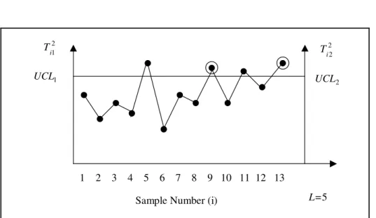
out-of-control period, Q=p. Figure 1 shows a SyTS bivariate control chart with the 2
1 i
T values
plotted. The 2
1 i
T point on the action region triggers the inspection of the whole sample, in
which case the statistic 2
2 i
T is computed and compared with UCL2. If Ti22>UCL2 then the
2 1 i
T point is surrounded by a circle. In other words, the nonconforming samples have their
2 1 i
T points surrounded by circles, see in Figure 1, 9th and 13th sample points. This simple
Sample Number (i)
1 2 3 4 5 6 7 8 9 10 11 12 13
1
UCL
2 1
i T
2
UCL
2 2
i T
L=5
Figure 1 – SyTS bivariate control chart with the 2
1 i
T values plotted.
When a process is in control, it is desirable that the expected number of samples taken since the beginning of the monitoring until a signal (ARL0) be large, to guarantee few false alarms.
When a process is out of control, it is desirable that the expected number of samples taken since the occurrence of the assignable cause until a signal (ARL) be small, in order to guarantee fast detection of process changes (see Costa et al. (2005)).
When the sampling interval is fixed, the ARL provides a measure of the time required to detect an assignable cause that is affecting the process since the beginning of the monitoring (zero-state ARL) or since the occurrence of the assignable cause (steady-state ARL). However, it is more realistic to assume that the assignable cause only occurs after the process has been running for some time. As a result, the assignable cause will occur between two nonconforming samples. The steady-state ARL measures how long the synthetic control chart will take to signal in this situation. We used the Markov chain model of the synthetic control chart described in Davis & Woodall (2002) to obtain the steady-state ARL for the SyTS bivariate chart.
The steady-state ARL values are presented in Table 1 for the synthetic bivariate chart with two-stage sampling, n=4, n0=9, UCL1=2.1973 and L=1, 5, 10, 20, 50, 100. As L increases
from 1 to 50, all the steady-state ARL values decrease. The process disturbance is measured
by λ= n(δ'x2+δ'y2), with
' 2 ' 2
x y
δ =δ . For example, if λ =0.5, the steady-state ARL
decreases from 84.79 to 59.74. The effect of varying L from 50 to 100 almost not affects the speed with which the chart detects small or large disturbances. For example, if λ =1.5, the steady-state ARL increases from 4.80 to 4.88 as L increases from 50 to 100. And if a larger shift is considered, for example, λ =3.0, the steady-state ARL decreases from 1.62 to 1.59 as L increases from 50 to 100. Table 1 also brings the ARL values for the standard bivariate chart (T2 chart). Inspection of Table 1 reveals that the SyTS Chart always outperforms the
2
T chart, except the case when L=1. For example, if λ =1.5 and L=20, the steady-state ARL
Table 1 – Effect of L on the steady-state ARL values for the SyTS chart. λ 2 T chart n=4 UCL=10.597 L=1 UCL2=3.380
L=5 UCL2=4.983
L=10 UCL2=5.635
L=20 UCL2=6.253
L=50 UCL2=7.001
L=100 UCL2=7.503
0.0 200.3 200.1 200.1 200.1 200.2 200.1 200.1
0.5 115.7 84.79 66.98 62.92 60.61 59.74 60.44
1.0 41.97 24.12 15.33 13.93 13.32 13.30 13.64
1.5 15.79 9.75 5.68 5.12 4.86 4.80 4.88
2.0 6.88 5.88 3.33 2.97 2.77 2.67 2.67
2.5 3.55 4.18 2.45 2.18 2.02 1.92 1.90
3.0 2.16 3.31 2.04 1.83 1.7 1.62 1.59
2 2
x
' ' y
n( )
λ= δ +δ , with 2 2
x
' ' y
δ =δ
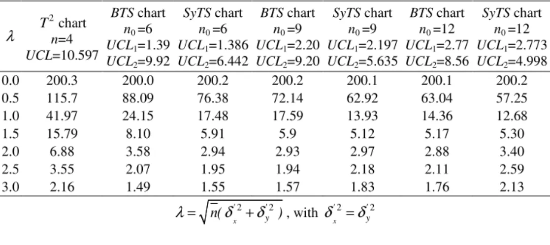
Table 2 brings the steady-state ARL values for the synthetic chart with two-stage sampling, 4
n= , L=10, and n0= 6, 9, 12. The choice of n0 affects the speed with which the SyTS chart
signals. Larger values of n0 are better for detecting smaller process changes and worse for detecting larger process changes. For example, one can see from Table 4 that, when λ =1.5, as n0 increases from 6 to 12, the steady-state ARL value decreases from 5.91 to 5.30. On the other hand, when λ =3.0, as n0 increases from 6 to 12, the steady-state ARL value increases
from 1.55 to 2.13. Table 2 also brings the ARL values for the standard bivariate chart T2 chart and the ARL values for the bivariate control chart with two-stage sampling (BTS chart). Inspection of Table 2 reveals the SyTS chart, when L=10, always outperforms the T2 chart and outperform the BTS chart for small disturbances. For example, if λ =1.0 and n0=9, the
steady-state ARL value for the SyTS chart is 13.93. The equivalent ARL values for the T2 chart and for the BTS chart are respectively 41.97 and 17.59. When λ increases from 1.5 to 3.0, most of the time the BTS chart has a better performance than the proposed chart (the SyTS chart). For example, if λ =2.5 and n0=9, the ARL value for the BTS chart is 1.94 and the steady-state ARL value for the SyTS chart is 2.18
Table 2 – Effect of n0 on the steady-state ARL values for the SyTS chart.
λ 2 T chart
n=4 UCL=10.597
BTS chart n0 =6 UCL1=1.39 UCL2=9.92
SyTS chart n0 =6 UCL1=1.386 UCL2=6.442
BTS chart n0 =9 UCL1=2.20 UCL2=9.20
SyTS chart n0 =9 UCL1=2.197 UCL2=5.635
BTS chart n0 =12 UCL1=2.77 UCL2=8.56
SyTS chart n0 =12 UCL1=2.773 UCL2=4.998
0.0 200.3 200.0 200.2 200.2 200.1 200.1 200.2 0.5 115.7 88.09 76.38 72.14 62.92 63.04 57.25 1.0 41.97 24.15 17.48 17.59 13.93 14.36 12.68
1.5 15.79 8.10 5.91 5.9 5.12 5.17 5.30
2.0 6.88 3.58 2.94 2.93 2.97 2.88 3.40
2.5 3.55 2.07 1.95 1.94 2.18 2.11 2.59
3.0 2.16 1.49 1.55 1.57 1.83 1.76 2.13
2 2
x
' ' y
n( )
λ= δ +δ , with 2 2
x
' ' y
4. Comparing charts
As the SyTS control chart was designed to detect small changes in the process parameters, it seems reasonable to compare its performance with the performance of the Hotelling’s T2 control chart with variable sample sizes (VSS chart).
The design of univariate Shewhart charts with adaptive sample sizes has been studied by Daudin (1992), Prabhu et al. (1993) and Costa (1994). Aparisi (1996) has extended these studies for the Hotelling’s T2 control chart. The monitoring procedure is as follows: the statistic Ti2=n(Xi− 0)' −1(Xi− 0) is charted with upper control limit UCLVSS. Two samples sizes are used, n1 and n2, n2>n1. A warning limit w is defined, where
0<w UCL< VSS as a threshold limit that identifies when to shift from one sample size to another (Fig. 2). The sample size of subgroup i depends on the value of Ti2−1. If
2 1
i
T− <w the ith subgroup sample size is n1, and corresponds to the black points in the chart. If
2 1
i VSS
w T< − <UCL the ith subgroup sample size is n2, and correspond to the white points in
the chart (see sample points 6, 8, 10 and 12). If Ti2>UCLVSS then the control chart signals.
VSS
UCL
w
Sample Number (i)
1 2 3 4 5 6 7 8 9 10 11 12 13
2
i T
Sample size n1 Sample size n2
Figure 2 – Hotelling’s T2 control chart with variable sample sizes.
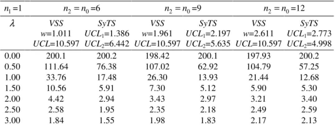
Table 3 provides the ARL for the SyTS chart and for the Hotelling’s T2 control chart with adaptive sample sizes. Similarly to Costa (1994), Aparisi (1996) obtained the ARL values for the Hotelling’s T2 control chart with adaptive sample sizes using Markov chains.
Table 3 – ARL values for the VSS and for the SyTS control charts with L=10 and n=4.
1
n =1 n2=n0=6 n2=n0=9 n2=n0=12
λ VSS
w=1.011 UCL=10.597
SyTS UCL1=1.386 UCL2=6.442
VSS w=1.961 UCL=10.597
SyTS UCL1=2.197 UCL2=5.635
VSS w=2.611 UCL=10.597
SyTS UCL1=2.773 UCL2=4.998
0.00 200.1 200.2 198.42 200.1 197.93 200.2 0.50 111.64 76.38 107.02 62.92 104.79 57.25
1.00 33.76 17.48 26.30 13.93 21.44 12.68
1.50 10.56 5.91 7.30 5.12 5.90 5.30
2.00 4.42 2.94 3.43 2.97 3.21 3.40
2.50 2.58 1.95 2.35 2.18 2.49 2.59
3.00 1.84 1.55 1.98 1.83 2.17 2.13
5. Illustrative example
In this section the proposed model is applied to the example considered by Montgomery (2004) to explain the use of the bivariate T2 control chart. The two quality characteristics are the tensile strength (psi) and the diameter of a textile fiber (x10-2 inch). He considered a set of twenty samples of size ten to estimate the in-control values of the mean vector and the covariance matrix:
0
115.59 1.06
= , 0 1.23 0.79
0.79 0.83
= .
Based on these estimations, ten samples of size n0+ 1, with n0= 6, were generated using the
DRNMVN sub routine available on the IMSL FORTRAN library (1995). After fixing n= 3,
the rate of inspected items per sampling, α = 0.005, the false alarm risk, and L = 2, the
expressions (6) and (11) were used to obtain the control chart limits, UCL1= 2.197 and
2
UCL = 4.911. The general expression of the Hotelling T2 statistic for two quality
characteristics is:
(
)
2(
)
2(
)(
)
2 2 2
2
y x x y xy y x
n
T ( n, )μμμμ = σ x−µ +σ y−µ − σ y−µ x−µ
According to the proposed sampling scheme, the sampling is performed in two stages. At the first stage, one item of the sample is inspected and the two correlated quality characteristics
( x; y ) are measured. The statistical distance between X'=( , )x y and '0=(µ0x;µ0y) is given by
(
)(
) (
)
(
)
(
)
(
)(
)(
)
2 2
2
1 2 1 1
1 1
1
[0.83 115.59 1.23 1.06
1.23 0.83 0.79
2 0.79 115.59 1.06 ]
T x y
x y
= − + −
−
− − −
If the statistic 2
1
T is lower than UCL1 the sampling is interrupted. Otherwise, the sampling
goes on to the second stage, where the remaining n0 items are inspected and the statistical
(
)(
) (
)
(
)
(
)
(
)
(
)(
)
2 2
2
2 2
7
[0.83 115.59 1.23 1.06
1.23 0.83 0.79
2 0.79 115.59 1.06 ]
T x y
x y
= − + −
−
− − −
is computed; being x and y the sample mean of the two correlated quality characteristics
( x; y ) taking into account the entire sample of size n0+ 1. When the statistic T22 is larger
than UCL2= 4.911, the sample is classified as nonconforming. According to the synthetic
procedure, the signal is based on the Conforming Run Length (CRL). The CRL is the number
of samples taken from the process since the previous nonconforming sample until the occurrence of the next nonconforming sample or, in case of the absence of previous
nonconforming sample, the CRL is the number of samples taken from the beginning of the
process monitoring until the occurrence of a nonconforming sample. The signal is given
when the CRL is smaller than or equal to L.
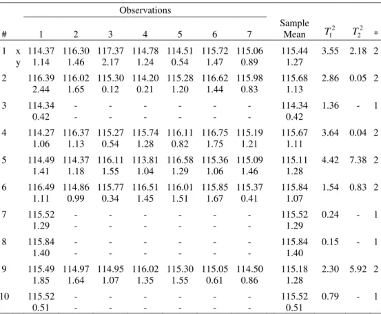
Table 4 presents the data of ( x; y ), the sample means, the statistics T12 and
2 2
T and the
sampling status.
Table 4 – Data for the illustrative example.
Observations
# 1 2 3 4 5 6 7
Sample Mean T12
2 2
T *
1 x 114.37 116.30 117.37 114.78 114.51 115.72 115.06 115.44 3.55 2.18 2 y 1.14 1.46 2.17 1.24 0.54 1.47 0.89 1.27
2 116.39 116.02 115.30 114.20 115.28 116.62 115.98 115.68 2.86 0.05 2 2.44 1.65 0.12 0.21 1.20 1.44 0.83 1.13
3 114.34 - - - 114.34 1.36 - 1
0.42 - - - 0.42
4 114.27 116.37 115.27 115.74 116.11 116.75 115.19 115.67 3.64 0.04 2 1.06 1.13 0.54 1.28 0.82 1.75 1.21 1.11
5 114.49 114.37 116.11 113.81 116.58 115.36 115.09 115.11 4.42 7.38 2 1.41 1.18 1.55 1.04 1.29 1.06 1.46 1.28
6 116.49 114.86 115.77 116.51 116.01 115.85 115.37 115.84 1.54 0.83 2 1.11 0.99 0.34 1.45 1.51 1.67 0.41 1.07
7 115.52 - - - 115.52 0.24 - 1
1.29 - - - 1.29
8 115.84 - - - 115.84 0.15 - 1
1.40 - - - 1.40
9 115.49 114.97 114.95 116.02 115.30 115.05 114.50 115.18 2.30 5.92 2 1.85 1.64 1.07 1.35 1.55 0.61 0.86 1.28
10 115.52 - - - 115.52 0.79 - 1
0.51 - - - 0.51
Figure 3 presents the SyTS control chart for the illustrative example. According to this figure,
the first nonconforming sample is the 5th sample, the second nonconforming sample is the
9th, and the CRL is equal four (9-5). As the CRL value is larger than L (= 2), the SyTS
bivariate control chart does not signal an out-of-control condition.
911 . 4 2 =
UCL
4,0
3,0
2,0
1,0
Sample Number (i)
1 2 3 4 5 6 7 8 9 10
2 1
i
T Ti22
L = 2
197 . 2
1 = UCL
Figure 3 – The SyTS control chart for tensile strength and diameter.
6. Conclusions
In this article, a synthetic control chart with two-stage sampling (SyTS chart) to control
bivariate processes was proposed for detecting assignable causes. An important advantage of the proposed chart is that the practitioner can control the process by looking at only one
chart. The synthetic control chart with two stage sampling (SyTS), the standard control chart,
the control chart with two-stage sampling and the VSS control charts for bivariate processes
were compared, in terms of the speed they detect changes in the process parameters. The
numerical results we obtained show a better overall performance of the SyTS chart if
compared with the other control charts.
In order to obtain the properties of the synthetic control chart with two-stage sampling, the IMSL FORTRAN library (1995) was used, where the subroutine DCSNDF is available to
evaluate the non-central chi-square distribution function. The SyTS chart was conceived to
attend the user because frequently they will be dealing with the situation where the inspection is reduced to the first item of the sample. Moreover, they feel more secure in stopping the process only after the occurrence of a second point beyond the control limits.
Acknowledgements
References
(1) Aparisi, F. (1996). Hotelling’s T2 control chart with adaptive sample sizes.
International Journal of Production Research, 34, 2853-2862.
(2) Aparisi, F. & Haro, C.L. (2001). Hotelling’s T2 control chart with variable sampling
intervals. International Journal of Production Research, 39, 3127-3140.
(3) Aparisi, F. & Haro, C.L. (2003). A comparison of T2 control charts with variable
sampling schemes as opposed to MEWMA chart. International Journal of Production
Research, 41, 2169-2182.
(4) Calzada, M.E. & Scariano, S.M. (2001). The robustness of the synthetic control chart to
non-normality. Communications in Statistics: Simulation and Computation, 30, 311-326.
(5) Champ, C.W. & Woodall, W.H. (1987). Exact results for Shewhart control charts with
supplementary runs rules. Technometrics, 29, 393-399.
(6) Chou, C.Y.; Chen, C.H. & Chen, C.H. (2006). Economic design of variable sampling
intervals T2 control charts using genetic algorithms.
Expert Systems with Applications,
30, 233-242.
(7) Costa, A.F.B. (1994). X charts with variable sample size. Journal of Quality
Technology, 26, 155-163.
(8) Costa, A.F.B. (1997). X charts with variable sample size and sampling intervals.
Journal of Quality Technology, 29, 197-204.
(9) Costa, A.F.B. (1998). Joint X and R charts with variable parameters. IIE Transactions,
30, 505-514.
(10) Costa, A.F.B. (1998a). Gráficos de controle X para processos robustos. Gestão&
Produção, 5, 259-271.
(11) Costa, A.F.B. (1999). Joint X and R charts with variable sample sizes and sampling
intervals. Journal of Quality Technology, 31, 387-397.
(12) Costa, A.F.B. (1999a). X charts with variable parameters. Journal of Quality
Technology,31, 408-416.
(13) Costa, A.F.B. & De Magalhães, M.S. (2007). An adaptive chart for monitoring the
process mean and variance. Quality and Reliability Engineering International (forthcoming).
(14) Costa, A.F.B. & Rahim, M.A. (2004). Joint X and R charts with two stage samplings.
Quality and Reliability Engineering-International, 20, 699-708.
(15) Costa, A.F.B. & Rahim, M.A. (2006). A synthetic control chart for monitoring the
process mean and variance. Journal of Quality in Maintenance Engineering, 12(1),
81-88.
(16) Costa, A.F.B. & Rahim, M.A. (2006a). The no-central chi-square chart with two stage
samplings. European Journal of Operational Research, 171, 64-73.
(17) Costa, A.F.B.; Epprecht, E.K. & Carpinetti, L.C.R. (2005). Controle Estatístico de
(18) Daudin, J.J. (1992). Double sampling X charts. Journal of Quality Technology, 24, 78-87.
(19) Davis, R.B. & Woodall, W.H. (2002). Evaluating and improving the synthetic control
chart. Journal of Quality Technology,34, 200-208.
(20) De Magalhães, M.S.; Epprecht, E.K. & Costa, A.F.B. (2001). Economic design of a VP
X chart. International Journal of Production Economics, 74, 191-200.
(21) De Magalhães, M.S.; Costa, A.F.B. & Epprecht, E.K. (2002). Constrained optimization
model for the design of an adaptive X chart. International Journal of Production
Research, 40, 3199-3218.
(22) De Magalhães, M.S. & Moura Neto, F.D. (2005). Joint economic model for totally
adaptive X and R charts. European Journal of Operational Research, 161, 148-161.
(23) De Magalhães, M.S.; Costa, A.F.B. & Moura Neto, F.D. (2006). Adaptive control
charts: a Markovian approach for processes subject to independent out-of-control
disturbances. International Journal of Production Economics, 99, 236-246.
(24) Epprecht, E.K. & Costa, A.F.B. (2001). Adaptive sample size control charts for
attributes. Quality Engineering,13, 465-473.
(25) Epprecht, E.K.; Costa, A.F.B. & Mendes, F.C.T. (2003). Adaptive control charts for
attributes. IIE Transactions,35, 567-582.
(26) Epprecht, E.K.; Costa, A.F.B. & Mendes, F.C.T. (2005). Gráficos de controle por
atributos e seu projeto na prática. Pesquisa Operacional,25, 113-134.
(27) Machado, M.A.G. & Costa, A.F.B. (2005). Synthetic control chart for monitoring the
process mean and variance. Proceedings of the XI International Conference on
Industrial Engineering and Operations Management, 1, 17-23.
(28) Michel, R. & Fogliatto, F.S. (2002). Projeto econômico de cartas adaptativas para
monitoramento de processos. Gestão&Produção, 9, 17-31.
(29) Microsoft Fortran Power Station 4.0. (1995). Professional Edition with Microsoft IMSL
Mathematical and Statistical Libraries. Microsoft Corporation.
(30) Montgomery, D.C. (2004). Introduction to Statistical Quality Control. John Wiley &
Sons, Inc., New York, New York.
(31) Prabhu, S.S.; Runger, G.C. & Keats, J.B. (1993). An adaptive sample size X chart.
International Journal of Production Research, 31, 2895-2909.
(32) Reynolds, M.R., Jr.; Amin, R.W.; Arnold, J.C. & Nachlas, J.A. (1988). X charts with
variable sampling intervals. TechnometricsI, 30, 181-192.
(33) Wexler, C. (1962). Analytic geometry: a vector approach. Addison-Wesley Publishing,
London.
(34) Wu, Z. & Spedding, T.A. (2000). A synthetic control chart for detecting small shifts in
the process mean. Journal of Quality Technology,32, 32-38.
(35) Wu, Z. & Spedding, T.A. (2000a). Implementing synthetic control charts. Journal of
(36) Wu, Z. & Yeo, S.H. (2001). Implementing synthetic control charts for attributes.
Journal of Quality Technology, 33, 112-114.
(37) Wu, Z.; Yeo, S.H. & Spedding, T.A. (2001). Implementing synthetic control charts.
Journal of Quality Technology, 33, 104-111.
(38) Yeh, A.B. & Lin, D.K.J. (2002). A new variables control chart for simultaneously
monitoring multivariate process mean and variability. International Journal of
Reliability, Quality and Safety Engineering, 9, 41-59.
Appendix: Theorem’s proof
Theorem A1: The random functions g ( n, )1 μμμμ and g ( n, )2 μμμμ have normal distribution with
zero mean vector and unit covariance matrix 1 0
0 1
= .
Proof: The random functions g ( n, )1 μμμμ and g ( n, )2 μμμμ are normal, because they are linear
combinations of normal variables xi and yi. We know that
2 2
( ) x
x E x
n σ µ
− = ,
2 2
( y) y
E y
n σ µ
− = , (E x x)(y xy) xy
n σ
µ µ
− − =
After some calculation we obtain
2 2
2 1
2
[ ( , )] n x y x y xysin cos
E g n
n n
σ σ
σ σ σ ϕ ϕ
= − .
By symmetry with respect to indices x and y, we have
2 2
2 2
1 2
1
[ ( , )] [ ( , )] x y x y xysin 2
n
E g n E g n
n n
σ σ
σ σ σ ϕ
= = −
As sin 2ϕ σ= xy/(σ σx y) and 2 2 2
xy
x y
σ σ σ
= − follows
2 2 2 2 2
1 2
1
[ ( , )] [ ( , )] 1
xy
x y
E g n =E g n = σ σ −σ =
Similarly
2 2
1 2
1
[ ( , ) ( , )] sin 2 sin 2 0
x y
x y xy x y
xy x y n
E g n g n
n n
σ σ σ σ σ
σ σ ϕ σ σ σ ϕ
= − = − =