Pesqui. Oper. vol.29 número3

MONITORING BIVARIATE PROCESSES

Marcela A. G. Machado* Antonio F. B. Costa Fernando A. E. Claro Production Department

São Paulo State University (UNESP) Guaratinguetá – SP, Brazil

marcela@feg.unesp.br fbranco@feg.unesp.br fernandoclaro@uol.com.br

* Corresponding author / autor para quem as correspondências devem ser encaminhadas

Recebido em 12/2008; aceito em 06/2009 Received December 2008; accepted June 2009

Abstract

The _T2 _{chart and the generalized variance |S| chart are the usual tools for monitoring the mean vector}

and the covariance matrix of multivariate processes. The main drawback of these charts is the difficulty to obtain and to interpret the values of their monitoring statistics. In this paper, we study control charts for monitoring bivariate processes that only requires the computation of sample means (the ZMAX chart) for monitoring the mean vector, sample variances (the VMAX chart) for monitoring the covariance matrix, or both sample means and sample variances (the MCMAX chart) in the case of the joint control of the mean vector and the covariance matrix.

Keywords: control charts; bivariate processes; mean vector; covariance matrix.

Resumo

Os gráficos de _T2 _{e da variância amostral generalizada |}

S| são as ferramentas usualmente utilizadas no monitoramento do vetor de médias e da matriz de covariâncias de processos multivariados. A principal desvantagem desses gráficos é a dificuldade em obter e interpretar os valores de suas estatísticas de monitoramento. Neste artigo, estudam-se gráficos de controle para o monitoramento de processos bivariados que necessitam somente do cálculo de médias amostrais (gráfico ZMAX) para o monitoramento do vetor de médias, ou das variâncias amostrais (gráfico VMAX) para o monitoramento da matriz de covariâncias, ou então das médias e variâncias amostrais (gráfico MCMAX) para o caso do monitoramento conjunto do vetor de médias e da matriz de covariâncias.

1. Introduction

The control charts are often used to observe whether a process is in control or not. When there is only one quality characteristic to control, the Shewhart charts are usually applied to detect process shifts. The power of the Shewhart control charts lies in its ability to separate the assignable causes of variation from the uncontrollable or inherent causes of variation. Shewhart control charts are relatively easy to construct and to interpret. As a result, they are readily implemented in manufacturing environments.

However, there are many situations in which it is necessary to control two or more related quality characteristics simultaneously. Hotelling (1947) provided the first solution to this problem by suggesting the use of the T2 statistic for monitoring the mean vector of multi-variate processes. Costa & Machado (2007) studied the properties of the synthetic T2 chart with two-stage sampling. Machado & Costa (2008a) considered the use of simultaneous

X charts as an alternative to the use of the T2 chart. Costa & Machado (2008a) considered the use of the double sampling procedure with the chart proposed by Hotelling.

The first multivariate control chart for monitoring the covariance matrix Σ was based on the charting statistic obtained from the generalized likelihood ratio test (Alt, 1985). For the case of two variables, Alt (1985) proposed the generalized variance statistic S to control the covariance matrix Σ.

Control charts more efficient than the S chart have been proposed. Recently, Costa & Machado (2008) considered the VMAX statistic to control the covariance matrix of bivariate processes. The points plotted on the VMAX chart correspond to the maximum of the sample variances of the two quality characteristics. Machado et al. (2008) obtained the properties of the VMAX chart with double sampling and Machado & Costa (2008) considered the EWMA chart based on the VMAX statistic. Costa & Machado (2008) extended the VMAX chart for the multivariate case, where p quality characteristics are under control. The synthetic VMAX chart for the bivariate case was also studied by Machado et al. (2009).

There are quite a few recent papers dealing with the joint control of the mean vector and the covariance matrix of multivariate processes. Khoo (2005) proposed a control chart based on the T2 and S statistics for monitoring bivariate processes. The speed with which the chart signals changes in the mean vector and/or in the covariance matrix was obtained by simulation. The results are not compelling, once the proposed chart is slow in signaling out-of-control conditions. Chen et al. (2005) proposed a single EWMA chart to control both, the mean vector and the covariance matrix. Their chart is more efficient than the joint T2 and S in signaling small changes in the process. Zhang & Chang (2008) proposed two EWMA charts based on individual observations that are not only fast in signaling but also very efficient in informing which parameter was affected by the assignable cause; if only the mean vector or only the covariance matrix or both. Machado & Costa (2008b) proposed the joint use of two charts based on the non-central chi-square statistic for monitoring the mean vector and the covariance matrix of bivariate processes, named as the joint NCS charts. In general, the joint NCS charts are faster than the combined T2 and S charts in signaling out-of-control conditions. Once the proposed scheme signals, the user can immediately identify the out-of-control variable.

This paper is organized as follows: the next section presents the assumptions and measure of efficiency. In Section 3, we present the ZMAX chart as an alternative to the T2 chart. In Section 4, we present the VMAX chart as an alternative to the S chart. In Section 5, we show the gain in speed with which the VMAX chart signals when the variable sample size, double sampling, synthetic or EWMA procedures are applied. In Section 6, we present the synthetic MCMAX chart as an alternative to the joint use of the T2 and S charts. Section 7 brings an illustrative example. Conclusions are in Section 8.

2. Assumptions and measure of efficiency

Throughout this article, it is assumed that the control charts are employed to monitor a bivariate process whose quality characteristics of interest (say, X and Y) are normally distributed with the mean vector µ and the covariance matrix Σ. The process is considered

to start with the mean vector and the covariance matrix on target ( 0

μ = μ

and Σ Σ= 0),

where '0 =(µ µx; y)

μ and 2 0 2 x xy xy y σ σ σ σ ⎛ ⎞ ⎜ ⎟ = ⎜_⎜ ⎟_⎟ ⎝ ⎠

Σ . Without losing generality we assume that

1.0

x y

σ =σ = . The T2 chart and the ZMAX chart are used to control processes that are

subject to assignable causes that change the mean vector from 0

μ

to '1=(µx+c;µy+d)

μ

,

where c and d measure the magnitude of the shift on each variable. The S chart and the VMAX chart are used to control processes that are subject to assignable causes that change

the covariance matrix from Σ₀ to

2 1 2 xy xy a ab ab b σ σ ⎛ ⎞ = ⎜_⎜ ⎟_⎟ ⎝ ⎠

Σ , where a and b measure the

increase in the variability of each variable. Finally, the joint T2 and S charts and the synthetic MCMAX are used to control processes that are subject to assignable causes that change the mean vector from μ₀ to μ₁ and/or change the covariance matrix from Σ₀ to Σ₁ without changing the correlation, that is, ρ σ= xy. The numerical results presented in this

paper are for the case of positive correlation, believed to be prevalent in industrial data.

The number of samples that are taken from the process until the control chart produces a signal measures the efficiency of a control chart. The expected number of samples taken before the chart signals is called the average run length (ARL). During the in-control period, ARL =1/α and is called ARL0. The risk α is the well known Type I error. The control limits of the

charts considered in this article were adjusted to assure a false alarm risk α = 0.005.

3. Control charts for monitoring the mean vector

A chart based on the sample means

1 / n

i i

X =

∑

1 / n

i i

Y =

∑

statistic ZMAX=max{ n X| −µx|, n Y| -µy|}, shortly ZMAX chart. A signal is given if ZMAX>CL, the control limit for the ZMAX chart. The power of the ZMAX chart is given by:

1 ( , ) _{x y}

CL c n CL d n

M x y Z Z

CL c n CL d n

P f Z Z d d

− −

− − − −

= −

∫

∫

where (f Z Zx, y) is a standardized bivariate normal distribution function with correlation ρ.

Table 1 – ARL values for the T2chart and for the ZMAX chart.

ρ

0.0 0.3 0.5 0.7

shifts ZMAX T2 ZMAX T2 ZMAX T2 ZMAX T2

c d CL 3.023 10.597 3.021 10.597 3.015 10.597 2.996 10.597

0.0 0.0 200.0 200.0 200.0 200.0 200.0 200.0 200.0 200.0

0.0 0.5 117.38 115.55 117.43 110.45 117.47 99.73 115.78 77.98

0.0 1.0 41.64 41.92 41.63 37.97 41.47 30.60 40.32 18.98

0.0 1.5 15.10 15.78 15.08 13.85 14.98 10.51 14.53 5.94

0.0 2.0 6.44 6.88 6.43 5.97 6.38 4.47 6.21 2.58

0.0 2.5 3.31 3.55 3.30 3.10 3.28 2.38 3.21 1.53

0.0 3.0 2.03 2.16 2.03 1.93 2.02 1.56 1.99 1.16

0.5 0.5 83.15 76.87 84.04 91.65 85.43 99.73 87.04 106.71

0.5 1.0 36.41 32.95 36.91 40.09 37.49 41.92 37.82 38.74

0.5 1.5 14.38 13.64 14.53 15.75 14.63 15.01 14.46 11.36

0.5 2.0 6.32 6.28 6.36 6.84 6.36 6.10 6.24 4.18

0.5 2.5 3.28 3.35 3.29 3.49 3.29 3.02 3.22 2.07

0.5 3.0 2.02 2.09 2.03 2.11 2.02 1.83 1.99 1.36

1.0 1.0 23.44 18.49 24.11 25.82 24.93 30.60 25.96 35.25

1.0 1.5 11.89 9.36 12.27 13.03 12.65 15.01 13.01 15.73

1.0 2.0 5.83 4.92 5.98 6.45 6.09 6.88 6.10 6.14

1.0 2.5 3.17 2.87 3.22 3.49 3.25 3.48 3.21 2.82

1.0 3.0 1.99 1.90 2.01 2.16 2.02 2.06 1.99 1.65

1.5 1.5 8.09 5.76 8.50 8.53 8.91 10.51 9.42 12.58

1.5 2.0 4.83 3.55 5.08 5.09 5.30 6.10 5.52 6.83

1.5 2.5 2.90 2.32 3.02 3.10 3.10 3.48 3.14 3.45

1.5 3.0 1.91 1.67 1.96 2.05 1.99 2.16 1.98 1.97

2.0 2.0 3.54 2.51 3.79 3.63 4.01 4.47 4.26 5.39

2.0 2.5 2.45 1.85 2.62 2.53 2.75 3.02 2.88 3.45

2.0 3.0 1.76 1.45 1.85 1.83 1.90 2.06 1.94 2.15

2.5 2.5 1.96 1.50 2.11 1.99 2.24 2.38 2.38 2.82

2.5 3.0 1.55 1.27 1.66 1.59 1.74 1.83 1.82 2.07

Table 1 brings the ARLs of the ZMAX and T2 charts. In terms of performance, the T2 chart is highly affected by the correlationρ, while ρ has a minor influence on the ZMAX chart. When the correlation is moderate (0.3-0.5) the ZMAX chart has a better overall performance (see ARL values in bold). Table 1 was built fixing n=5 and ARL0 = 200.0. The study with

other n values led to the same conclusions.

4. Monitoring the covariance matrix

A chart based on the sample variances S_x2 =

∑

(

)

∑

(

)

is considered to control Σ. As an alternative to the use of two S2 charts we consider a single chart based on the statistic VMAX=max{S2_x,S2_y}, shortly VMAX chart. A signal is given if VMAX>CL, the control limit for the VMAX chart. According to Costa & Machado (2008), the power of the VMAX chart is given by:

(

)

₍

₎

₍

₎

S n n

nCL

P _t e t dt

n b ρ ρ χ ρ − − − ⎡ ⎤ ⎢ ⎥

= − <

Γ

⎢ ₋ ⎥

⎣ ⎦

∫

Recalling that the notation χn m2, represents a non-central chi-square distribution with n

degrees of freedom and non-centrality parameter given by m. We used the subroutine

DCSNDF available on the Microsoft Fortran library (1995) to compute the non-central

chi-square distribution function.

In this section we compare the ARL for the VMAX chart with the ARL for the S chart (the generalized variance S chart) proposed by Alt (1985). When the process is in control,

(

)

0

2⋅ − ⋅n 1 S / Σ is distributed as a chi-square with 2n−4 degrees of freedom. The

covariance matrix S is given by xx xy

yx yy s s s s ⎡ ⎤ = ⎢ ⎥ ⎣ ⎦

S , being sxx and syy the sample variances of

X and Y and sxy and syx, the sample covariances. The control limit for the S chart is:

(

)

(

)

2 2

2 4, 0

2 4 1 n CL n α

χ ₋ ⋅

=

⋅ − Σ

. (3)

One drawback of the S chart is that the user is not familiar with the computation of sample covariances and determinants of covariances matrixes.

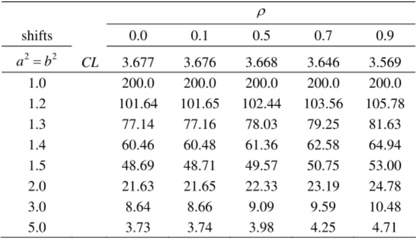
The S chart’s performance is independent of ρ, while ρ has some influence on the

Table 2 – The influence of the correlation on the VMAX chart’s performance (values of ARL).

ρ

shifts 0.0 0.1 0.5 0.7 0.9

2 2

a =b CL 3.677 3.676 3.668 3.646 3.569

1.0 200.0 200.0 200.0 200.0 200.0

1.2 101.64 101.65 102.44 103.56 105.78

1.3 77.14 77.16 78.03 79.25 81.63

1.4 60.46 60.48 61.36 62.58 64.94

1.5 48.69 48.71 49.57 50.75 53.00

2.0 21.63 21.65 22.33 23.19 24.78

3.0 8.64 8.66 9.09 9.59 10.48 5.0 3.73 3.74 3.98 4.25 4.71

Table 3 – The ARL for the S and VMAX charts.

n

4 5

shifts S VMAX S VMAX

2 2

a =b CL 6.134 4.094 5.375 3.668

1.0 200.0 200.0 200.0 200.0

1.2 112.48 107.00 104.60 102.44

1.3 89.13 82.90 80.45 78.03

1.4 73.30 66.14 64.08 61.36

1.5 60.35 54.10 51.91 49.57

2.0 30.24 25.42 24.11 22.33

3.0 13.64 10.72 10.16 9.09

5.0 6.37 4.77 4.58 3.98

4.1 Description of the VMAX chart with variable sample size

The idea of varying the size of the samples was introduced by Costa (1994) and, since then, it has been considered with a variety of control charts (see for instance, Aparisi (1996), Aparisi et al. (2001) and Epprecht & Costa (2001)). According to this procedure, random samples of variable sizes are taken from the process every h hours. The sample values are plotted on a control chart with warning limit WLi and action limit CLi, depending on the

sample size n_i, i=1, 2, where n₂ >n₁.

The size of each sample depends on the sample point position of the preceding sample. If the sample point falls in the central region, that is, VMAX<WLi, then the next sample size

should be n₁, and if the sample point falls in the warning region, that is,

VMAX

i i

The properties of a control chart with VSS are also determined by the number of samples that are taken from the process until the control chart produces a signal. We suppose that the

process remains in control with Σ=Σ₀ for a long time until the occurrence of the

assignable cause. After the assignable cause occurrence the covariance matrix changes, that is, Σ=Σ₁. During the in-control period, the rate of inspected items per sampling, n, is given by

(

)

1 0 2 1 0

n=n p +n −p (4)

being p₀ the probability of a sample point falling in the central region, given that it did not fall in the action region.

When the process is out-of-control, the ARL is obtained using Markov chains (see Costa & Machado (2008) for details).

4.2 The VMAX chart with double sampling

When the double sampling (DS) scheme is in use samples of size n=n₁+n₂ are taken from the process at regular time intervals. The sampling is performed in two stages. At the first stage n₁ items are inspected and their quality characteristics (X;Y) are measured. With the

sample variances of (X;Y) the VMAX1 is computed, that is, VMAX1= max{S12x,S12y}.

If VMAX1<WL, the sampling is interrupted and the process is considered in control, where

WL is the warning limit for the first stage. The control chart signals an out-of-control

condition when VMAX1>CL1, where CL1 is the control limit for the first stage,

1 0

CL >WL> . If WL<VMAX₁≤CL₁, the sampling goes on to the second stage, where the

remaining n2 items of the sample are inspected and the

2 2

2 2 2

VMAX =max{S x,S y} statistic is

computed, being S2x2 and 2 2y

S the sample variances of (X;Y) considering the whole sample

of size n. The control chart also signals an out-of-control condition when VMAX2>CL2,

where CL₂ is the control limit for the second stage.

If the chart produces a signal when the process is operating properly with Σ Σ= 0, this

signal is a false alarm. At the first stage the false alarm risk is given by α₁ and, at the second stage, it is given by α2.

If the chart signals after the occurrence of the assignable cause, that is, when Σ Σ≠ ₀, this signal is a true alarm. At the first stage the power of the chart detecting an assignable cause is given by p1 and, at the second stage, it is given by p2.

This way, when the DSprocedure is in use, the false alarm risk and the power of the VMAX chart are given by α α α= 1+ 2 and p= p1+p2, respectively.

During the in-control period, the rate of inspected items per sampling, n, is given by:

1 2(1- 0)

where p0 is the probability that the DS procedure ends at the first stage, that is

[

]

0 1 Pr VMAX1 1

p = − WL< <CL . (6)

When the DS procedure is in use, the average run length (ARL) also measures the efficiency of a control chart in detecting a process change. The expression to obtain the ARL for the VMAX chart with DS is shown in Machado & Costa (2008).

From earlier studies (Daudin, 1992), we observed that the charts with DS perform better with

1

CL = ∞, that is, α1=0. In this case, a VMAX1 point in the region above WL always

triggers the inspection of the whole sample.

4.3 The synthetic VMAX chart

According to the synthetic procedure (see Wu & Spedding, 2000), the signal is based on the Conforming Run Length (CRL). The CRL is the number of samples taken from the process since the previous nonconforming sample until the occurrence of the next nonconforming

sample. In the case of the absence of a previous nonconforming sample, the CRL is the

number of samples taken from the beginning of the monitoring until the occurrence of a

nonconforming sample. The signal is given when the CRL≤L, where L is a specified

positive integer.

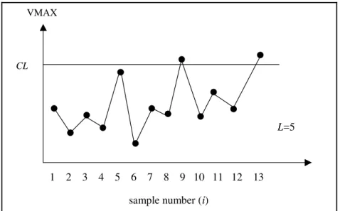
Figure 1 shows the synthetic VMAX chart. The sample is classified as nonconforming when VMAXi falls beyond the control limit CL. Samples 9 and 13 are nonconforming (Figure 1).

In this case, CRL = 4 (13th sample – 9th sample = 4). As CRL < L (=5), the synthetic VMAX chart signals an out-of-control condition.

VMAX

sample number (i)

1 2 3 4 5 6 7 8 9 10 11 12 13

CL

L=5

For many types of control charts (for instance, the Shewhart chart), the ARL value for a given shift in the mean and/or in the variance of the process does not depend on whether the assignable cause is affecting the process since the beginning of the monitoring

(zero-state ARL) or whether it only occurs after the process has been running for some time

(steady-stateARL) that is, the zero-state ARL and the steady-state ARL are equal. However,

for charts based on conforming run lengths, such as synthetic charts, this does not happen. We assume that the assignable cause only occurs after the process has been running for some time, so the performance measure will be the steady-state ARL.

Davis & Woodall (2002) obtained the steady-state ARL (SSARL) through a Markov chain model. We adopted this approach to obtain the steady-state ARL (SSARL) for the synthetic VMAX chart, see Machado et al. (2009) for details.

4.4 The EWMA scheme based on the VMAX statistic

The EWMA chart we propose to detect changes in the covariance matrix

Σ

(

)

VMAX 1

i i i

Z =λ + −λ Z− , i = 1,2,…, (7)

where VMAX max{ 2, 2}

i i

i= Sx Sy , being

2

i

x

S and 2

i

y

S the sample variances of X and Y, and λ

is a smoothing parameter, satisfying 0< ≤λ 1. The value of λ determines the weight given to the current sample value. When λ=1 the EWMA places all of it weights on the most recent observation. The starting value Z0 is often taken to be the expected in-control value

of Z (see Lucas & Saccucci, 1990). A signal is given if Z_i>CL, the control limit for the EWMA chart.

For the EWMA chart, the expected length of time from the process change to the signal will depend on the value of the control statistic Z at the time the change occurs. We assume that the control statistic has reached its steady-state or stationary distribution by the random point in time that the change occurs. When the steady-state distribution is adopted the chart’s performance is measured by the steady-state ARL, shortly SSARL. Machado & Costa (2008) used the Markov chain approach described in Saccucci & Lucas (1990) to obtain the

SSARL values.

5. Comparing charts

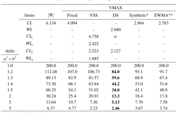
Table 4 – The ARL values for the S chart and for the VMAX charts

(ρ= 0.5, n = 4, n1= 3 and n2= 12).

VMAX

limits S Fixed VSS DS Synthetic* EWMA**

CL 6.134 4.094 - - 2.964 2.783

WL - - - 2.680 - -

1

CL - - 4.758 ∞ - -

1

WL - - 2.425 - - -

shifts CL2 - - 2.523 2.127 - -

2 2

a =b WL2 - - 1.685 - - -

1.0 200.0 200.0 200.0 200.0 200.0 200.0

1.2 112.48 107.0 106.73 84.0 93.1 91.7

1.3 89.13 82.9 81.57 59.6 68.9 67.4

1.4 73.30 66.1 63.84 44.2 53.0 51.6

1.5 60.35 54.1 51.02 34.0 42.1 40.9

2 30.24 25.4 20.91 13.3 18.4 17.8

3 13.64 10.7 7.36 5.13 7.70 7.58

5 6.37 4.77 3.23 2.46 3.67 3.74

*L=5; **λ=0.5

From Table 4 we conclude that the VMAX chart with DS is the one with the best performance (see the ARL in bold).

6. Control charts for monitoring the mean vector and the covariance matrix

A chart based on the sample means X =

∑

∑

variances Sx =

∑

(

)

2

2 _µ

and Sy =

∑

(

)

2

2 _µ

is considered to control μ

and

Σ

chart, where Zx= n X( −µx), Zy= n Y( −µy),

2

x x

W =kS and Wy=kSy2. The parameter k

is required to attend the imposed condition that, during the in-control period, the four statistics (|Zx|, |Zy|,Wx,Wy) have the same probability to exceed CL, the control limit of the proposed chart. The power of the MCMAX chart is given by

M S M S

P=P +P ′−P P ′. (8)

where

(

)

2

2 2 ( 1)

2 2 [( 1) / 2] 1

2 2 ( 1) 2 , 1

0

( 1) 1

1 Pr

(1 ) 2 [( 1) / 2]

n CL

t n ka

S n t n

n CL

P e t dt

kb n ρ ρ χ ρ − − − − ′ − − ⎡ − ⎤

= − _⎢ < _⎥

− Γ −

⎣ ⎦

and PM is given by expression (1). The control limit CL is obtained by expression (1), with

c = d = 0 and P_M = −1 1−α . The value of k is obtained by expression (9), with a = b = 1

and PS′ = −1 1−α . We used a grid search to obtain CL and k.

The sample points plotted on the MCMAX chart correspond to the largest value among (|Z_x|, |Z_y|,W_x,W_y). The MCMAX chart is not always faster in signaling than the joint T2

and S charts. However, the synthetic procedure improves the performance of the MCMAX

chart. According to this procedure, a second sample point beyond the upper control limit and not far than L sampling intervals from the first one triggers the alarm.

We also adopted the approach proposed by Davis & Woodall (2002) to obtain the ARL for the synthetic MCMAX chart.

Table 5 shows the influence of the design parameter L on the MCMAX performance. As L

increases the speed with which the synthetic MCMAX chart signals also increases. The gain in speed is more significant when L increases from 1 to 6. For instance, when a = b = 1 and

c = d = 0.5, the ARL reduces 18.0 % (from 21.4 to 17.5). By other hand, as L increases from 6 to 10, the ARL reduces 1.0 % (from 17.5 to 17.3).

Table 5 – The influence of the L value on the synthetic MCMAX chart’s performance (n=5 andρ= 0.5).

L

shifts 1 2 3 4 5 6 7 8 9 10

a b c d CL 2.350 2.469 2.536 2.582 2.617 2.644 2.667 2.687 2.703 2.719

1.0 1.0 0 0 200.0 200.0 200.0 200.0 200.0 200.0 200.0 200.0 200.0 200.0 0 0.5 45.3 40.9 39.1 37.9 37.3 36.8 36.3 36.1 35.9 35.7

0.5 0.5 21.4 19.2 18.4 17.9 17.7 17.5 17.4 17.3 17.3 17.3

1.25 1.25 0 0 13.6 12.0 11.3 11.0 10.8 10.8 10.6 10.6 10.6 10.6

0 0.5 8.9 7.8 7.3 7.1 7.0 7.0 6.9 6.9 6.9 6.9

0.5 0.5 6.5 5.7 5.4 5.3 5.2 5.2 5.2 5.1 5.1 5.1

1.5 1.0 0 0 10.1 8.5 7.9 7.5 7.3 7.3 7.1 7.0 7.0 7.0

0 0.5 7.6 6.5 6.1 5.9 5.8 5.8 5.7 5.7 5.7 5.7

0.5 0 7.2 6.0 5.6 5.3 5.2 5.2 5.0 5.0 5.0 4.9

0.5 0.5 5.8 5.0 4.7 4.5 4.4 4.4 4.3 4.3 4.3 4.3

Table 6 presents the ARLs of both the synthetic MCMAX chart and the joint T2 and S charts. The synthetic MCMAX chart is faster in signaling than the joint charts, except when the correlation between X and Y is high. When the correlation is high, the joint charts are, in general, faster in signaling assignable causes that only affect the mean and/or the variability

of one of the two quality characteristics. We chose the usual sample size n=5. The

Table 6 – ARL values of the joint T2 and S charts and the synthetic MCMAX chart (n=5 and L = 7).

Shifts (mean vector) Shifts (covariance

matrix) c 0 0 0.5 0.5 0 0.75 0.75 0 1.0 1.0

a b ρ d 0 0.5 0 0.5 0.75 0 0.75 1.0 0 1.0

1.0 1.0 0.0 200.0 48.9* 49.2 19.9 16.7 16.8 5.4 6.8 6.6 2.3

200.0 36.3** 36.3 17.4 10.8 10.8 5.1 4.3 4.3 2.3

0.5 200.0 38.4* 38.5 34.8 10.8 10.8 10.6 4.1 4.2 4.1

200.0 36.3** 36.3 17.4 10.8 10.8 5.1 4.3 4.3 2.3

0.7 200.0 20.6* 20.2 39.7 5.7 5.6 12.9 2.3 2.3 5.0

200.0 36.3** 36.3 17.4 10.8 10.8 5.1 4.3 4.3 2.3

1.25 1.0 0.0 42.6 22.2 17.5 11.0 11.2 8.9 4.4 5.2 4.7 2.1

28.2 15.0 12.1 8.6 7.3 6.2 3.8 3.7 3.5 2.1

0.5 41.6 17.7 14.1 15.8 7.6 6.6 7.1 3.5 3.5 3.5

26.5 14.4 11.7 8.4 7.2 6.1 3.8 3.6 3.5 2.1

0.7 39.1 11.9 9.8 17.1 4.6 4.2 8.2 2.2 2.2 4.1

25.1 14.0 11.4 8.2 7.1 6.0 3.8 3.6 3.6 2.1

1.5 1.0 0.0 15.3 10.7 9.0 6.7 6.9 5.8 3.5 4.0 3.7 2.0

7.5 5.9 5.2 4.5 4.2 3.8 3.8 2.8 2.7 1.9

0.5 14.6 8.9 7.7 8.4 5.2 4.6 5.0 3.0 2.9 3.0

7.1 5.7 5.0 4.3 4.1 3.7 2.8 2.7 2.7 1.9

0.7 13.1 6.9 5.8 8.3 3.6 3.4 5.3 2.0 2.1 3.3

6.7 5.5 4.9 4.2 4.0 3.6 2.7 2.7 2.6 1.9

1.25 1.25 0.0 15.6 9.9 9.8 6.8 6.2 6.3 3.5 3.9 3.9 2.0

10.2 6.7 6.7 5.0 4.4 4.4 2.9 2.9 2.9 1.9

0.5 15.9 8.7 8.6 8.6 4.9 4.8 4.9 2.9 2.9 2.9

10.6 6.9 6.9 5.1 4.5 4.5 3.0 2.9 2.9 1.9

0.7 15.7 6.9 6.8 9.2 3.5 3.5 5.4 2.0 2.0 3.3

11.2 7.2 7.2 5.3 4.6 4.6 3.0 3.0 3.0 1.9

1.5 1.5 0.0 4.4 3.6 3.6 3.1 3.0 3.0 2.3 2.4 2.4 1.7

3.0 2.6 2.6 2.4 2.3 2.3 1.9 1.9 1.9 1.6

0.5 4.3 3.5 3.5 3.4 2.7 2.7 2.7 2.1 2.1 2.1

3.2 2.8 2.8 2.5 2.4 2.4 2.0 2.0 2.0 1.6

0.7 4.3 3.1 3.1 3.6 2.3 2.3 2.9 1.7 1.7 2.2

3.4 2.9 2.9 2.6 2.5 2.5 2.0 2.0 2.0 1.6

7. Illustrative example

The purpose of the following example is to show the ability of the synthetic MCMAX chart in detecting shifts in the mean vector and/or in the covariance matrix. To this end, we considered a bivariate process whose quality characteristics of interest, X and Y, are normally distributed. When the process is in-control, the mean vector and the covariance matrix are

given by µ'₀ =(0, 0) and ₀ 1 0

0 1

⎛ ⎞

= ⎜ ⎟

⎝ ⎠

Σ .

We initially generate 5 samples of size 5 with the process in control. The last 5 samples were simulated considering that the assignable cause changes the mean and the variability of X, that is, µx=1.0 and σx=1.25.

Table 7 presents the data of X, Y, Z, W and MCMAX. The control limit of CL = 2.667 was determined by expression (1), with c=d=0, to assure a false alarm risk α of 0.005.Figure 2 shows the synthetic MCMAX control chart. As the number of sampling intervals l (=2) is smaller than L (=7), the synthetic MCMAX control chart signals an out-of-control condition.

Table 7 – Values of X, Y, Z, W and MCMAX (L=7).

Sample Z W_{* MCMAX}

1 X _{-0.284 -0.467 -0.067 0.875 0.188 0.110 0.049 1.204}

Y _{-0.457 -0.758 -0.709 -0.332 -0.436 1.204 0.006}

2 0.213 1.624 -0.781 -1.26 0.273 0.031 0.221 0.518

-2.741 0.525 0.078 1.96 0.036 0.064 0.518

3 -1.51 0.247 0.355 -1.187 1.026 0.478 0.209 0.478

0.034 2.198 -1.369 -0.234 0.243 0.390 0.297

4 2.275 0.179 0.125 -1.685 -0.917 0.010 0.397 0.397

0.987 -1.154 -0.302 0.437 0.857 0.369 0.142

5 -0.086 0.999 -0.741 -0.755 0.799 0.097 0.123 0.619

0.29 2.512 -0.143 -0.693 -0.581 0.619 0.305

6 -0.706 1.381 2.096 -0.021 1.891 2.076 0.270 2.076

0.18 -1.093 1.35 1.527 -1.286 0.303 0.309

7 0.117 2.042 -0.725 2.679 0.45 2.041 0.353 2.041

1.027 0.75 -0.214 -0.186 2.047 1.531 0.158

8 1.489 1.652 1.438 1.193 1.691 3.338 0.007 3.338

0.565 -0.115 -0.868 0.899 0.19 0.300 0.082

9 0.725 0.066 1.183 0.632 2.135 2.120 0.107 2.120

0.866 -0.668 -0.242 2.329 0.029 1.035 0.250

10 2.468 -2.009 3.845 3.552 0.918 3.924 1.023 3.924

0 1 2 3 4

1 2 3 4 5 6 7 8 9 10

Sample number (i)

MCMAX

CL=2.667

Figure 2 – The synthetic MCMAX chart – example.

8. Conclusions

In this article we proposed new charts to control the mean vector and/or the covariance matrix of bivariate processes. The monitoring statistics associated to these charts are based on the sample means and sample variances. As the control chart’s users are, in general, more familiar with means and variances, they will have less difficult to deal with the proposed charts if compared with the charts proposed by Hotelling (1947) and Alt (1985). In terms of efficiency, the VMAX chart always performs better than the S chart. With the rule of the two points beyond the control limit, the synthetic MCMAX chart almost ever performs better than the joint T2 and S charts.

Acknowledgements

This work was supported by CNPq – National Council for Scientific and Technological Development, Project 307744/2006-0 – and FAPESP – The State of São Paulo Research Foundation, Project 2006/00491-0. We are in debt with the three anonymous referees who carefully read an earlier draft and made many constructive suggestions. During the celebration of the 40th SBPO event, this paper was elected the best one in the field of Operations Management. We would like to thank the award committee.

References

(1) Alt, F.B. (1985). Multivariate quality control. In: Encyclopedia of Statistical Science

[edited by S. Kotz and N.L. Johnson], 6, 110-122.

(2) Aparisi, F. (1996). Hotelling’s T2 control chart with adaptive sample sizes. International

Journal of Production Research, 34, 2853-2862.

(3) Aparisi, F.; Jabaloyes, J. & Carrión, A. (2001). Generalized variance chart design with adaptive sample sizes. The bivariate case. Communication in Statistics – Simulation and

(4) Chen, G.; Cheng, S.W. & Xie, H. (2005). A new multivariate control chart for monitoring both location and dispersion. Communications in Statistics-Simulation and

Computation,34, 203-217.

(5) Costa, A.F.B. (1994). X control charts with variable sample size. Journal of Quality

Technology, 26, 155-163.

(6) Costa, A.F.B. & Machado, M.A.G. (2007). Synthetic control charts with two-stage

sampling for monitoring bivariate processes. Pesquisa Operacional, 27, 117-130.

(7) Costa, A.F.B. & Machado, M.A.G. (2008). A new multivariate control chart for

monitoring the covariance matrix of bivariate processes. Communications in

Statistics-Simulation and Computation, 37, 1453-1465.

(8) Costa, A.F.B. & Machado, M.A.G. (2008a). Bivariate control charts with double

sampling. Journal of Applied Statistics, 35, 809-822.

(9) Costa, A.F.B. & Machado, M.A.G. (2009). A new chart based on sample variances for monitoring the covariance matrix of multivariate processes. International Journal of

Advanced Manufacturing Technology, 41, 770-779.

(10) Daudin, J.J. (1992). Double sampling X charts. Journal of Quality Technology, 24, 78-87.

(11) Davis, R.B. & Woodall, W.H. (2002). Evaluating and improving the synthetic control chart. Journal of Quality Technology, 34, 200-208.

(12) Epprecht, E.K. & Costa, A.F.B. (2001). Adaptive sample size control charts for

attributes. Quality Engineering, 13, 465-473.

(13) Hotelling, H. (1947). Multivariate quality control, illustrated by the air testing of sample bombsights. Techniques of Statistical Analysis, 111-184.

(14) Khoo. B.C. (2005). A new bivariate control chart to monitor the multivariate process mean and variance simultaneously. Quality Engineering, 17, 109-118.

(15) Lucas, J.M. & Saccucci, M.S. (1990). Exponentially weighted moving average control schemes: properties and enhancements. Technometrics, 32, 1-16.

(16) Machado, M.A.G. & Costa, A.F.B. (2008). The double sampling and the EWMA charts based on the sample variances. International Journal of Production Economics, 114, 134-148.

(17) Machado, M.A.G. & Costa, A.F.B. (2008a). Some comments on the use of principal components and simultaneous univariate control charts for multivariate process control.

Pesquisa Operacional,28, 173-196.

(18) Machado, M.A.G. & Costa, A.F.B. (2008b). Monitoring the mean vector and the

covariance matrix of bivariate processes. Brazilian Journal of Operations and

Production Management, 5, 47-62.

(19) Machado, M.A.G.; De Magalhães, M.S. & Costa, A.F.B. (2008). Gráfico de controle de VMAX para o monitoramento da matriz de covariâncias. Produção, 18, 222-239.

(20) Machado, M.A.G.; Costa, A.F.B. & Rahim, M.A. (2009). The synthetic control chart

based on two sample variances for monitoring the covariance matrix. Quality and

(21) Microsoft Fortran Power Station 4.0 (1995). Professional Edition with Microsoft IMSL

Mathematical and Statistical Libraries. Microsoft Corporation, Washington, USA.

(22) Saccucci, M.S. & Lucas, J.M. (1990). Average run lengths for exponentially weighted moving average control schemes using the Markov chain approach. Journal of Quality

Technology,22, 154-162.

(23) Zhang, G. & Chang, S.I. (2008). Multivariate EWMA control charts using individual observations for process mean and variance monitoring and diagnosis. International

Journal of Production Research, 46, 6855-6881.