www.hydrol-earth-syst-sci.net/15/1937/2011/ doi:10.5194/hess-15-1937-2011
© Author(s) 2011. CC Attribution 3.0 License.
Earth System
Sciences
Trend analysis of extreme precipitation in the Northwestern
Highlands of Ethiopia with a case study of Debre Markos
H. Shang1, J. Yan1,2, M. Gebremichael3, and S. M. Ayalew4
1Department of Statistics, University of Connecticut, Storrs, Connecticut, USA
2Center for Environmental Sciences and Engineering, University of Connecticut, Storrs, Connecticut, USA 3Department of Civil and Environmental Engineering, University of Connecticut, Storrs, Connecticut, USA 4Department of Civil Engineering, Faculty of Technology, Addis Ababa University, Ethiopia
Received: 21 September 2010 – Published in Hydrol. Earth Syst. Sci. Discuss.: 28 October 2010 Revised: 28 March 2011 – Accepted: 13 June 2011 – Published: 24 June 2011
Abstract. Understanding extreme precipitation is very im-portant for Ethiopia, which is heavily dependent on low-productivity rainfed agriculture but lacks structural and non-structural water regulating and storage mechanisms. There has been an increasing concern about whether there is an increasing trend in extreme precipitation as the climate changes. Existing analysis of this region has been descrip-tive, without taking advantage of the advances in extreme value modeling. After reviewing the statistical methodology on extremes, this paper presents an analysis based on the generalized extreme value modeling with daily time series of precipitation records at Debre Markos in the Northwest-ern Highlands of Ethiopia. We found no strong evidence to reject the null hypothesis that there is no increasing trend in extreme precipitation at this location.
1 Introduction
In Ethiopia, rainfall is by far the most important factor cli-mate, as is true for most of Africa. Low-productivity agricul-ture, which accounts for a majority of the national economy, relies heavily on rainfall. Climate extremes such as drought or flood often lead to famine and disaster for the vulnerable agricultural, social and economic environment in Ethiopia, which lacks structural and non-structural water regulating
Correspondence to:J. Yan (jun.yan@uconn.edu)
and storage mechanisms. In particular, flood, as a result of extreme precipitation, poses serious threat on food security and public safety. Estimating the probability of extreme pre-cipitation and characterizing the uncertainty of the estimates are crucial to, for instance, structural design, public safety alerts, evacuation management, and loss mitigation.
Given the increasing public concern on climate change, it is of particular interest to test whether there is a long term increasing trend in extreme precipitation. Studies have been done for different parts of the world. For examples, Kunkel et al. (1999) reported an increasing trend in the United States at a rate of 3 % per decade from 1931 to 1996, but no significant trend during 1951–1993 in Canada; Kunkel (2003) showed a sizeable increase in the frequency of ex-treme precipitation events since the 1920s/1930s in the US; Frei and Sch¨ar (2001) found an increase in the frequency of heavy precipitation during 1901–1994 in the Alpine region of Switzerland; Goswami et al. (2006) detected a significant ris-ing trend in both the frequency and the magnitude of extreme rainfall events from 1951 to 2000 in central India; Karagian-nidis et al. (2009) reported no significant trend in extreme precipitation of the European continent from the mid 1970’s to 2000.
based on a binomial model for the counts. Zhang et al. (2004) compared three methods for trend detection in extreme val-ues in a Monte Carlo study, ordinary least squares regression, nonparametric Mann-Kendall test, and generalized extreme value (GEV) modeling. The GEV method can use the m -largest observations each year. Explicit GEV modeling was found to always outperform the other two methods, and the use ofm-largest observations was found to improve the de-tection power for moderate values ofm.
Rainfall patterns in Ethiopia have been reported in previ-ous studies. A decline of annual and summer rainfall in east-ern, southeast-ern, and southwestern Ethiopia was found, but no trend was detected over central, northern, and northwestern Ethiopia (Seleshi and Zanke, 2004; Cheung et al., 2008). It is worth noting, however, that annual or summer total rainfall and annual maximum daily rainfall are very different aspects of rainfall characterization. Seleshi and Camberlin (2006) studied changes in extreme seasonal rainfall as measured by extreme rainfall indices with daily rainfall data. One of the indices was extreme intensity, defined as the average inten-sity of events greater than or equal to the 95th percentile. A weak increasing trend in summer extreme intensity over the 10–11◦North band of the Ethiopia Highlands and no trend was found over the remaining Highlands, based on the non-parametric Mann-Kendall test for trend. These existing anal-yses have been descriptive, without taking advantage of the advances in extreme value modeling from the statistics liter-ature. To the best of our knowledge, extreme value analysis based on the GEV modeling has not been applied to extreme precipitation data in Ethiopia.
The GEV distribution was first introduced by Fisher and Tippett (1928) as limits of the sample maximum or minimum for independent, identically distributed variables. Extreme value theory has evolved into a proliferating field in statis-tics, motivated by numerous environmental applications. Ac-cessible statistical references are, for instances, Coles (2001) and Beirlant et al. (2004). Extreme precipitation has been an important application area of extreme value analysis (e.g., Durman et al., 2001; Kharin and Zwiers, 2005; Huerta and Sans´o, 2007). In particular, statistical inferences for univari-ate extreme value analysis, as is the case with the precipi-tation data at a single location, have been rather mature and widely applied by practitioners in many fields. Two standard approaches can be used to fit a univariate GEV distribution. The first one, known as the block maxima approach, applies to annual maxima of a time series, using only one data point, the maximum, per year. The second one applies to all ex-ceedances over a high threshold, also known as “peaks over threshold” (POT). The method we adopted in this article is a variant of the POT approach, the point process approach; see Sect. 3 for more details. Compared to them-largest observa-tion approach, which can be wasteful if one block happens to contain more extreme events than another, the point process approach utilizes more information from the data. Given the
proach is adopted in this application as it takes full advantage of daily precipitation record in fitting GEV distributions.
Through GEV models, this article aims to provide an ex-treme value analysis of the annual maximum precipitation in Debre Markos, Ethiopia. Specifically, our objective is to test whether there is an increasing trend in extreme precipitation in this area given the public concerns of suspected trend as a consequence of global climate changes. We incorporated a linear function of time in the location parameter of a GEV distribution and fitted the model with the POT approach to the daily precipitation data at Debre Markos. No evidence was found to support an increasing trend in extreme precipi-tation since 1953 at this location.
The rest of the article is organized as follows. Details of the data are described in Sect. 2. The statistical methods to be used, including the extreme value theory and modeling tech-niques, are reviewed in Sect. 3. The results of the extreme value analysis are reported in Sect. 4 with a test for trend. A discussion concludes in Sect. 5.
2 Data
Debre Markos is a city in the Blue Nile River basin on the Northwestern Highlands of Ethiopia. It has latitude 10◦20′N, longitude 37◦43′E, and elevation 2446 m. Al-though the topography of Ethiopia is highly diverse, more than 45 % of the country is dominated by highlands with elevations greater than 1500 m, where almost 90 % of the nation’s population resides. The rain gauge station at De-bre Markos provides the longest record among all stations in Ethiopia. Daily precipitation records are available from 1953, with only a tiny proportion of missing data. We use Debre Markos as a case study to investigate the long term trend in extreme precipitation in the Northwestern highland of Ethiopia.
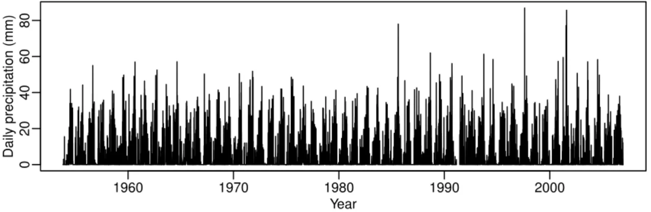
Our raw data of daily precipitation at Debre Markos spans from 1 November 1953 to 10 December 2006. Out of the to-tal of 19 398 days, 229 (about 1.2 %) observations are miss-ing. The observed daily time series of precipitation is plotted in Fig. 1. The maximum daily was 86.9 mm, observed on 14 August 1997.
Year
Daily precipitation (mm)
1960 1970 1980 1990 2000
0
20
40
60
80
Fig. 1.Times series of daily precipitation at Debre Markos, Ethiopia.
● ●●●●●●●● ●● ●● ● ● ● ●● ● ●●● ● ● ●●●●● ● ●● ●● ● ● ● ● ● ●●● ●●● ● ● ●●●● ● ●●●● ● ● ● ● ● ● ● ● ● ● ● ● ●● ● ●●● ● ● ●● ●● ● ● ●●● ● ● ● ● ● ● ●● ● ● ● ● ●● ●● ●●●● ● ● ● ● ● ● ● ●● ●● ● ● ● ●● ● ● ● ● ● ● ● ● ● ● ● ●● ● ● ● ● ● ●● ● ●● ●● ● ●● ●● ● ● ● ● ● ● ● ● ● ● ● ● ● ● ● ● ● ● ● ● ● ● ● ● ● ● ●● ● ●●● ● ● ● ● ●●● ● ● ● ● ● ●●● ● ● ● ●● ● ● ●● ● ● ● ● ● ● ● ● ●● ● ● ● ● ●● ● ● ● ● ● ● ● ● ● ● ● ● ● ● ● ● ● ● ● ● ● ● ● ● ● ● ●● ● ● ● ●● ● ● ● ● ● ● ● ● ● ● ● ● ● ● ● ● ● ● ● ● ● ● ● ●● ● ● ● ● ● ● ● ● ● ● ● ● ● ● ● ● ● ● ● ● ● ●● ● ● ● ● ● ● ● ● ● ● ● ●●● ● ●● ● ●●●●●●●● ●● ●●●● ● ●● ● ●● ●●●● ● ● ●● ● ● ● ●●● ● ●● ● ●●●● ● ● Month A ver
age Precipitation f
or all y
ears (mm)
1 2 3 4 5 6 7 8 9 10 12
0 2 4 6 8 10 12 ● ● ● ● ● ● ● ● ● ● ● ●
2 4 6 8 10 12
5 10 15 20 25 30 Month Threshold f
or each month (mm)
Fig. 2. Left: scatter plot of mean precipitation for each day overlaid with the 11-day moving average. Right: threshold chosen for each month.
than 5 %, which confirms that there is temporal dependence and hence the declustering is necessary.
Strong seasonality naturally exists in the data. As most areas in Ethiopia, there are three seasons in Debre Markos: main rainy season (June to September), dry season (October to January), and small rainy season (February to May), which are locally known as Kiremt, Bega, and Belg, respectively. Figure 2 (left panel) shows the mean precipitation for each day in a year, with the 11-day moving average overlaid. The plot is consistent with the three seasons. High precipitations are observed in summer months and low precipitations are observed in winter months. Our extreme value analysis needs to take the clustering and seasonality into account.
3 Methods
The basis of extreme value modeling is the GEV distribution, with distribution function
F (z;µ,σ,ξ )= (
exp
n −
1+ξ z−σµ−1/ξ
o
,ξ6=0, 1+ξ z−σµ
>0,
exp
−exp
−z−σµ ,ξ=0, (1)
whereµ∈R is a location parameter, σ >0 is a scale pa-rameter, andξ ∈Ris a shape parameter governing the tail behavior. The Gumbel family is the limiting case ofξ→0. The sub-families defined byξ >0 andξ <0 correspond to the Fr´echet family and the Weibull family, respectively. The
m-yr return levelzm, with the return period 1/m, is
calcu-lated fromF (zm)=1−1/m. When the only available data
is a sequence of annual maxima of daily precipitation, the maximum likelihood approach can be applied to make in-ferences about the unknown parameters. Usual regularity conditions of the maximum likelihood estimator are satisfied
the point process approach are more attractive in that all ex-ceedances over threshold, instead of just the annual max-ima, contribute to the inference. Assuming thatX1,...,Xn
are independent and identically distributed, Pickands (1971) showed that, for sufficiently large thresholdu, the sequence of point processes{(i/(n+1),Xi):i=1,...,n}is
approxi-mated by a Poisson process on the region(0,1)×[u,∞)with intensity function onA=(t1,t2)× [z,∞)given by
3(A)=nx(t2−t1)
1+ξ
z−µ
σ
−1/ξ
, (2)
wherenx is the number of years of data to which the
avail-ableXicorrespond, ensuring that the parameters(µ,σ,ξ )are
the same as those in the GEV approximation (Eq. 1) of an-nual maxima. The point process approach is adopted because the parameter estimates are not directly tied to the choice of thresholduand the ideal threshold is determined by consid-ering the smallestu beyond which the parameter estimates stabilize.
Suppose that we observekexceedances of daily precipita-tion over thresholdu,x1,...,xk, fromnxyear’s of data. The
likelihood function is
L(µ,σ,ξ;x1,...,xk)=
exp (
−nx
1+ξ
u−µ σ
−1/ξ) k Y
i=1 σ−1
1+ξ
xi−µ
σ
−1/ξ−1 . (3) The point process likelihood is based on all data greater thanu, thus inferences are likely to be more accurate than estimates based on the classical GEV model which studies only block maxima. The likelihood also takes into account of missing data in that where there are missing data,nxwill be the number of year’s worth of observed data.
So far we have assumed that the data are independent and identically distributed, which is clearly violated in the daily series data. Before we can apply the likelihood function, we need to remove the clustering and seasonality from the ob-served data.
We use runs algorithm to filter the dependent observa-tions to obtain a set of threshold excesses that are approx-imately independent (Smith and Weissman, 1994). For a given threshold, define clusters to be wherever there are con-secutive exceedances of this threshold. In particular, two ex-ceedances of the threshold that are separated apart by fewer thanrobservations are deemed part of the same cluster. That is, only after a certain number,r, of observations fall below the threshold, the cluster is terminated. In practice, it is rec-ommended to try differentr values for comparison (Smith, 1989; Mannshardt-Shamseldin et al., 2010).
To handle the seasonality, we adopt a simple and broadly applicable approach that allows all model parameters of the Poisson process to be seasonally dependent. Specifically, we allow each month to have its own GEV parameters as in Smith (1989).
value of threshold can be arbitrary to some extent for initial analysis, too low a threshold is likely to violate the asymp-totic basis of the model and too high a threshold will lead to too few exceedances for data analysis. An exploratory tool for choosinguis the mean residual life plot (e.g., Coles, 2001, Ch. 4). When u is sufficiently large, the expected residual life,E(X−u|X > u), is a linear function ofu. In a mean residual life plot, we plot the sample mean residual life against thresholdu, and choose the smallest u beyond which the mean residual life plot is approximately linear.
4 Results
The mean residual plots with 95% confidence intervals are drawn for each month with run lengthr=1 in Fig. 3. For all months, the figures are approximately linear when the thresh-old exceeds the sample 95% percentile. Therefore, we take the 95% percentile as threshold for each month. This is dif-ferent from the analysis of Smith (1989), where the same threshold was used for all months. The right panel of Fig. 2 shows the thresholds we choose for each month, which has similar pattern as the average precipitation plot in the left panel.
Each month is modeled separately, thus no specific form describing the seasonal variation is assumed. Letµij,σij
andξij denote the GEV parameters for month j of year i.
To detect the long-term trend for each month, we assume the form
µij=αj+iβj, σij=σj>0, ξij=ξj, (4)
where the location parameterµij includes a linear trend in
year with coefficientβj. This form was also adopted to detect
trend by Smith (1989) with ground-level ozone and by Coo-ley (2009) with annual maximum temperatures. The likeli-hoodLj of monthj,j=1,...,12, is maximized separately to estimate(αj,βj,σj,ξj).
It turns out that none of theβj parameters is significant at 5 % level, indicating there is no strong evidence of long-term increasing trend over time. The models are re-fitted with allβj=0. The sum of the maximized log likelihood is−3063.91 for the models in all 12 months, which is very close to that with βj’s in the model (−3060.29). The
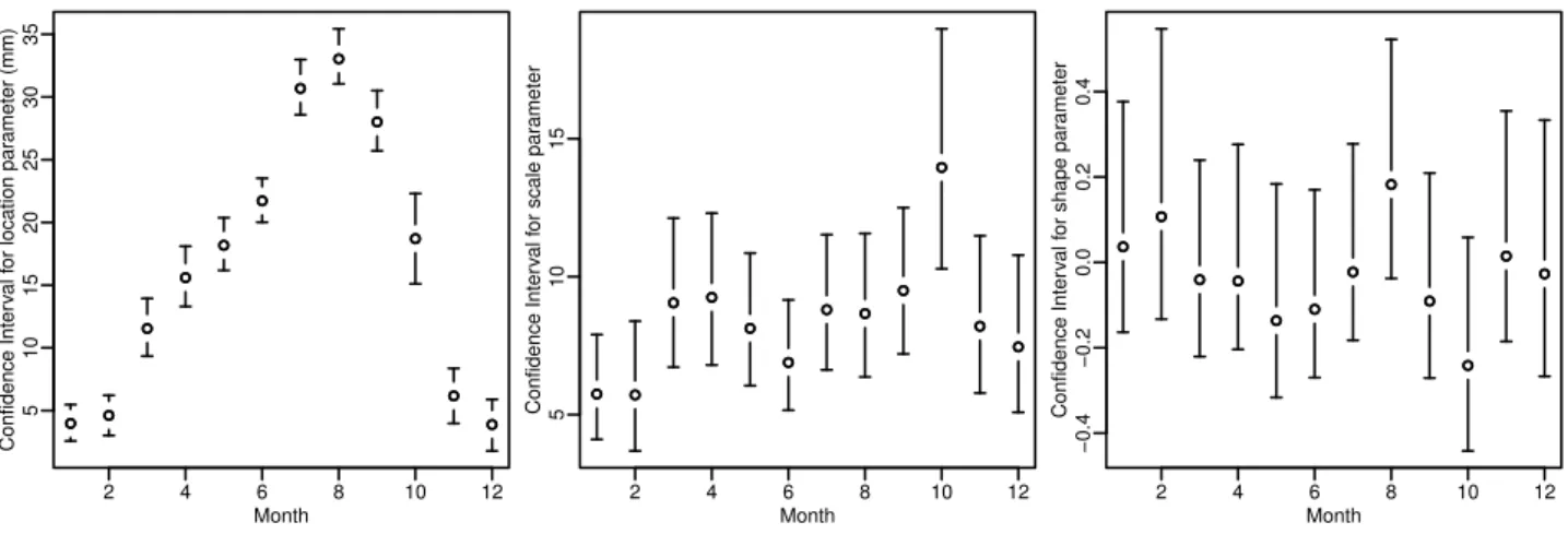
pa-rameter estimates with no trend are shown in Table 1. There is strong seasonal pattern for the location parameterµ. The other parametersσ andξ, however, vary haphazardly. All
ξ’s are estimated greater than−0.5, indicating that the esti-mators are regular and they have the usual asymptotic prop-erties. The 10-yr return level for each specific month, calcu-lated from GEV distribution, is also shown in the table.
The 95 % confidence intervals for parameter estimates are calculated by profile likelihood (Coles, 2001, Ch. 2), which is shown in Fig. 4. Although the confidence interval ofξ
0 2 4 6 8 10 12
2
3
4
5
6
7
8
9
Threshold in January (mm)
Mean e
xcess (mm)
85%90% 95%
0 2 4 6 8 10 12
4
6
8
10
Threshold in February (mm)
Mean e
xcess (mm)
85% 90% 95%
0 5 10 15 20
4
6
8
10
12
Threshold in March (mm)
Mean e
xcess (mm)
85% 90% 95%
0 5 10 15 20 25 30
2
4
6
8
10
12
Threshold in April (mm)
Mean e
xcess (mm)
85%90% 95%
0 5 10 15 20 25
4
6
8
10
Threshold in May (mm)
Mean e
xcess (mm)
85% 90% 95%
0 5 10 15 20 25 30
2
4
6
8
10
12
14
Threshold in June (mm)
Mean e
xcess (mm)
85% 90% 95%
0 10 20 30 40
5
10
15
20
25
30
Threshold in July (mm)
Mean e
xcess (mm)
85%90% 95%
0 10 20 30 40
5
10
15
20
25
30
35
Threshold in August (mm)
Mean e
xcess (mm)
85%90% 95%
0 10 20 30
5
10
15
Threshold in September (mm)
Mean e
xcess (mm)
85% 90% 95%
0 5 10 15 20 25 30 35
4
6
8
10
12
14
Threshold in October (mm)
Mean e
xcess (mm)
85% 90% 95%
0 5 10 15
4
6
8
10
12
14
Threshold in November (mm)
Mean e
xcess (mm)
85%90% 95%
0 2 4 6 8 10 12 14
4
6
8
10
12
Threshold in December (mm)
Mean e
xcess (mm)
85%90% 95%
● ● ●
● ●
● ●
●
●
● ●
2 4 6 8 10 12
5
10
15
20
25
30
Month
Confidence Inter
val f
or location par
ameter (mm)
● ● ●
● ●
● ●
●
●
● ●
● ● ● ●
●
● ● ●
● ●
● ●
2 4 6 8 10 12
5
10
15
Month
Confidence Inter
val f
or scale par
ameter
● ● ● ●
●
● ● ●
● ●
● ●
● ●
● ●
● ●
● ●
●
● ●
●
2 4 6 8 10 12
−0.4
−0.2
0.0
0.2
0.4
Month
Confidence Inter
val f
or shape par
ameter
● ●
● ●
● ●
● ●
●
● ●
●
Fig. 4.95% confidence intervals for GEV parameters. Left: confidence intervals forµ. Middle: confidence intervals forσ. Right: confidence intervals forξ.
Table 1.Parameter estimates and standard errors for each month with no trend.
Month Number of µ σ ξ 10-yr return
Exceedances level
1 65 3.97 (0.74) 5.74 (0.96) 0.04 (0.14) 17.45
2 56 4.61 (0.77) 5.71 (1.20) 0.11 (0.17) 19.15
3 67 11.54 (1.17) 9.05 (1.35) −0.04 (0.12) 31.00
4 68 15.60 (1.20) 9.25 (1.38) −0.04 (0.12) 35.42
5 69 18.18 (1.05) 8.13 (1.21) −0.14 (0.13) 33.92
6 67 21.72 (0.88) 6.89 (1.01) −0.11 (0.11) 35.46
7 72 30.68 (1.12) 8.80 (1.23) −0.02 (0.11) 50.00
8 75 33.04 (1.12) 8.66 (1.34) 0.18 (0.14) 57.14
9 73 28.01 (1.21) 9.50 (1.34) −0.09 (0.12) 47.34
10 66 18.71 (1.80) 13.96 (2.17) −0.24 (0.13) 42.94
11 60 6.17 (1.07) 8.20 (1.46) 0.01 (0.14) 24.94
12 57 3.89 (0.99) 7.45 (1.44) −0.03 (0.15) 20.16
Gumbel model with constraintξ=0, because “a reduction to the Gumbel subfamily is always risky” (Coles and Pericchi, 2003, p. 416); the uncertainty in parameterξ would other-wise be inappropriately accounted for.
To check the sensitivity of results to the choice of threshold
uand run lengthr, return levels are compared under different choices. Since there is seasonality during the year, the calcu-lation of the return level can be derived through the maxima for each month. LetM1,...,M12denote the maxima for each
month. Them-yr return levelzmwill satisfy 1−1
m =
Pr{max(M1,...,M12)≤zm}
=
12
Y
i=1
exp (
−
1+ξi
z
m−µi
σi
−1/ξi)
. (5)
The confidence interval for return level can be obtained by simulation. We simulate the model parameters first from
the the multivariate normal approximation of the estimator. For each set of generated parameters, a realization of the re-turn level is obtained by solving Eq. (5). A large number (N=5000) of realizations is used to approximate the confi-dence intervals.
Table 2 summarizes the parameter estimates and 95% con-fidence intervals for 10-yr, 50-yr and 100-yr return levels for different combinations of(u,r). It appears that the inference is quite robust on the choice ofr for all return levels. The inference on the 10-yr return level is robust to the choice of
Table 2.Estimated return levels and their 95 % confidence intervals under different choices for thresholduand run lengthr.
u r 10-yr return level 50-yr return level 100-yr return level
Q85 % 1 69.0 (64.6, 78.4) 90.0 (82.3, 117.6) 100.5 (91.3, 147.8) Q85 % 2 69.0 (64.5, 78.5) 89.8 (81.8, 118.5) 100.1 (89.6, 154.0) Q90 % 1 68.6 (63.5, 79.0) 91.4 (82.0, 122.8) 103.4 (90.8, 154.6) Q90 % 2 68.5 (63.3, 78.7) 90.6 (80.9, 119.6) 102.0 (88.7, 146.6) Q95 % 1 68.4 (61.7, 80.8) 97.2 (80.5, 142.2) 113.4 (89.5, 186.5) Q95 % 2 68.4 (61.8, 80.5) 96.8 (80.0, 141.3) 112.7 (89.8, 184.0) Q97 % 1 68.1 (61.3, 81.2) 99.3 (79.6, 155.4) 118.0 (90.1, 223.4) Q97 % 2 67.9 (61.1, 80.1) 98.3 (78.5, 153.4) 116.4 (88.0, 208.9)
Among all those threshold sets, the only significantβj’s were found when u=Q90 % andr=1, with standardized
beta values−2.07 and−2.15 for February and July, respec-tively. We conclude that there is no increasing long-term trend for any month.
As a model diagnosis, we performed goodness-of-fit test for the GEV distribution with the annual maximum daily pre-cipitation data in each of the 12 months over 53 yr. There were 10, 10, and 13 zeros in January, February, and De-cember, respectively. These zeros were removed to run the goodness-of-fit test as, otherwise, a distribution with point mass at zero would be needed and any continuous distribu-tion would fail to capture this. For the POT approach, these zeroes would not affect the result as they do not affect the selection of the threshold. Thep-values of the Kolmogorov-Smirnov test statistic are, respectively, 0.405, 0.220, 0.197, 0.127, 0.674, 0.621, 0.562, 0.560, 0.313, 0.465, 0.494, and 0.372 from January to December, suggesting no lack of fit from the GEV distribution. Thep-values of the Anderson-Darling test give similar results.
Finally, we present the estimated return level plots for the model with no trend in Fig. 5. The 95 % confidence intervals were obtained again by a large number (N=5000) of Monte Carlo simulation that accounts for the uncertainty in param-eter estimate. The 100-yr return level was estimated as 96.4, with a 95 % confidence interval(78.7,161.0).
5 Conclusions
With the extreme value theory, we presented a case study with the daily precipitation series at Debre Markos, Ethiopia. No evidence was found to support long-term increasing trend in extreme precipitation at this location. This means, for in-stance, that the 100-yr return level has not increased signifi-cantly during the period of 1953–2006. We have performed the same analysis with daily records separately at two other sites, Bahir Dar and Gondar, in the Blue Nile River basin on the Northwestern Highland in Ethiopia. No significant trend was found at either sites.
In practice, for a given data set, many parametric fami-lies may fit the data well and pass the goodness-of-fit test.
Return period (Years)
Retur
n le
vel (mm)
1 5 10 100 1000
50
100
150
200
●●●●●●●●●●●●●● ●●●●●●●●●●●●●●●●●●●●●●●●
●●●● ●●●●● ●● ●
●
● ●
Fig. 5. Return levels (solid line) with 95 % confidence intervals (dashed lines) obtained from 5000 Monte Carlo simulation. The circles are the empirical estimates based on the observed 53-yr’s data.
GEV. These distributions, however, can differ very much in tails, which is what we want to study through extreme value analysis. For this reason, a GEV model may be preferred as it is by definition the limit distribution of sample maximums. Our current extreme value analysis deals one site at a time. It cannot address important questions that involve events jointly defined across multiple sites; for instance, what is the probability that the 100-yr return levels of three sites in the vicinity of a city occur in the same year? Estimating the probability of extremal events at a network of locations with spatial dependence appropriately accounted is a much more challenging problem. Spatial extremes is a new and rapidly developing field (e.g., Cooley et al., 2007; Padoan et al., 2010). Further extreme analysis in a spatial context for Ethiopia, with data from a network of sites, is worth investi-gating.
Acknowledgements. H. Shang and J. Yan were partially supported
by a grant from the University of Connecticut Research Foundation. M. Gebremichael was partially supported by NASA NIP Grant No. NNX08AR31G and NASA Grant No. NNX10AG77G to the University of Connecticut.
Edited by: A. Melesse
References
Beirlant, J., Goegebeur, Y., Segers, J., and Teugels, J.: Statistics of Extremes: Theory and Applications, John Wiley & Sons Inc, 2004.
Cheung, W. H., Senay, G. B., and Singh, A.: Trends and Spatial Distribution of Annual and Seasonal Rainfall in Ethiopia, Int. J. Climatol., 28, 1723–1734, 2008.
Coles, S.: An Introduction to Statistical Modeling of Extreme Val-ues, Springer-Verlag Inc, 2001.
Coles, S. and Pericchi, L.: Anticipating Catastrophes through Ex-treme Value Modelling, J. Roy. Stat. Soc. C-App., 52, 405–416, 2003.
Cooley, D.: Extreme Value Analyis and the Study of Climate Change: A Commentary on Wigley 1988, Clim. Change, 97, 77– 83, 2009.
Cooley, D., Nychka, D., and Naveau, P.: Bayesian Spatial Modeling of Extreme Precipitation Return Levels, J. Am. Stat. Assoc., 102, 824–840, 2007.
Durman, C. F., Gregory, J. M., Hassell, D. C., Jones, R. G., and Murphy, J. M.: A Comparison of Extreme European Daily Pre-cipitation Simulated by a Global and a Regional Climate Model for Present and Future Climates, Q. J. Roy. Meteor. Soc., 127, 1005–1015, 2001.
Fisher, R. A. and Tippett, L. H. C.: Limiting Forms of the Frequency Distributions of the Largest or Smallest Member of a Sample, P. Camb. Philos. Soc., 24, 180–190, 1928.
Alpine Region, J. Climate, 14, 1568–1584, 2001.
Goswami, B. N., Venugopal, V., Sengupta, D., Madhusoodanan, M. S., and Xavier, P. K.: Increasing Trend of Extreme Rain Events over India in a Warming Environment, Science, 314, 1442–1445, 2006.
Huerta, G. and Sans´o, B.: Time-varying Models for Extreme Val-ues, Environ. Ecol. Stat., 14, 285–299, 2007.
Karagiannidis, A., Karacostas, T., Maheras, P., and Makrogiannis, T.: Trends and Seasonality of Extreme Precipitation Character-istics related to Mid-latitude Cyclones in Europe, Adv. Geosci., 20, 39–43, doi:10.5194/adgeo-20-39-2009, 2009.
Kharin, V. V. and Zwiers, F. W.: Estimating Extremes in Transient Climate Change Simulations, J. Climate, 18, 1156–1173, 2005. Kullback, S.: The Kullback-Leibler Distance [Letter], The
Ameri-can Statistician, 41, 340–341, 1987.
Kunkel, K. E.: North American Trends in Extreme Precipitation, Nat. Hazards, 29, 291–305, 2003.
Kunkel, K. E., Andsager, K., and Easterling, D. R.: Long-Term Trends in Extreme Precipitation Events over the Conterminous United States and Canada, J. Climate, 12, 2515–2527, 1999. Mannshardt-Shamseldin, E. C., Smith, R. L., Sain, S. R., Mearns,
L. O., and Cooley, D.: Downscaling Extremes: A Comparison of Extreme Value Distributions in Point-source and Gridded Pre-cipitation Data, The Annals of Applied Statistics, 4, 484–502, 2010.
Padoan, S. A., Ribatet, M., and Sisson, S. A.: Likelihood-based In-ference for Max-stable Processes, J. Am. Stat. Assoc., 105, 263– 277, 2010.
Pickands, J.: The Two-dimensional Poisson Process and Extremal Processes, J. Appl. Probab., 8, 745–756, 1971.
Seleshi, Y. and Camberlin, P.: Recent Changes in Dry Spell and Extreme Rainfall Events in Ethiopia, Theor. Appl. Climatol., 83, 181–191, 2006.
Seleshi, Y. and Zanke, U.: Recent Changes in Rainfall and Rainy Days in Ethiopia, Int. J. Climatol., 24, 973–983, 2004.
Smith, R. L.: Maximum Likelihood Estimation in a Class of Non-regular Cases, Biometrika, 72, 67–90, 1985.
Smith, R. L.: Extreme Value Analysis of Environmental Time Se-ries: An Application to Trend Detection in Ground-level Ozone (C/R: P378-393), Stat. Sci., 4, 367–377, 1989.
Smith, R. L. and Weissman, I.: Estimating the Extremal Index, J. Roy. Stat. Soc. B, 56, 515–528, 1994.
Vuong, Q. H.: Likelihood Ratio Tests for Model Selection and Non-nested Hypotheses (STMA V31 0456), Econometrica, 57, 307– 333, 1989.
White, H.: Maximum Likelihood Estimation of Misspecified Mod-els, Econometrica, 50, 1–26, 1982.