Subtle leakage of a Majorana mode into a quantum dot
E. Vernek,1,2P. H. Penteado,2A. C. Seridonio,3and J. C. Egues2
1Instituto de F´ısica, Universidade Federal de Uberlˆandia, Uberlˆandia, Minas Gerais 38400-902, Brazil 2Instituto de F´ısica de S˜ao Carlos, Universidade de S˜ao Paulo, S˜ao Carlos, S˜ao Paulo 13560-970, Brazil 3Departamento de F´ısica e Qu´ımica, Universidade Estadual Paulista, Ilha Solteira, S˜ao Paulo 15385-000, Brazil
(Received 15 August 2013; revised manuscript received 10 April 2014; published 30 April 2014) We investigate quantum transport through a quantum dot connected to source and drain leads and side coupled to a topological superconducting nanowire (Kitaev chain) sustaining Majorana end modes. Using a recursive Green’s-function approach, we determine the local density of states of the system and find that the end Majorana mode of the wire leaks into the dot, thus, emerging as a unique dot levelpinnedto the Fermi energyεF of the leads. Surprisingly, this resonance pinning, resembling, in this sense, a “Kondo resonance,” occurs even when the gate-controlled dot levelεdot(Vg) is far above or far belowεF. The calculated conductanceGof the dot exhibits an unambiguous signature for the Majorana end mode of the wire: In essence, an off-resonance dot [εdot(Vg)=εF], which should haveG=0, shows, instead, a conductancee2/2hover a wide range ofV
gdue to this pinned dot mode. Interestingly, this pinning effect only occurs when the dot level is coupled to a Majorana mode; ordinary fermionic modes (e.g., disorder) in the wire simply split and broaden (if a continuum) the dot level. We discuss experimental scenarios to probe Majorana modes in wires via these leaked/pinned dot modes.
DOI:10.1103/PhysRevB.89.165314 PACS number(s): 71.10.Pm,03.67.Lx,74.25.F−,74.45.+c
I. INTRODUCTION
Zero-bias anomalies in transport properties are one of the most intriguing features of the low-temperature physics in nanostructures. The canonical example is the zero-bias peak in the conductance of interacting quantum dots (QDs) coupled to metallic contacts, which is a clear manifestation of the Kondo effect [1,2] arising from the dynamical screening of the unpaired electron spin in the quantum dot by the itinerant electrons of the leads. Another example is the Andreev bound state arising from electron and hole scatterings at a normal-superconductor interface [3].
Recently, a new type of zero-bias anomaly has emerged in connection with the appearance of Majorana bound states in Zeeman-split nanowires with spin-orbit interaction in close proximity to ans-wave superconductor [4,5]. It is theoretically well established that these “topological” superconducting wires sustain chargeless zero-energy end states with peculiar features, such as braiding statistics, possibly relevant for topo-logical quantum computation [6,7]. Experimentally, however, there is still controversy as to what the observed zero-bias peak really means: Kondo effect, Andreev bound states, and disorder effects are some of the possibilities [8–15]. Franz summarizes and discusses these issues in Ref. [16].
Here we propose a direct way to probe the Majorana end mode arising in a topological superconducting nanowire by measuring the two-terminal conductance G through a dot side coupled to the wire, Figs.1(a)and1(b). Using an exact recursive Green’s-function approach, we calculate the LDOS of the dot and wire and show that the Majorana end mode of the wire leaks into the dot [17], thus, giving rise to a Majorana resonance in the dot, Figs.1(c)and1(d). Surprisingly, we find that this dot-Majorana mode is pinned to the Fermi levelεF
of the leads even when the gate-controlled dot levelεdot(Vg) is
far off-resonanceεdot(Vg)=εF.
Based on the results above, we suggest three experimental ways for probing the Majorana end mode in the wire via the leaked/pinned Majorana mode in the dot: (i) with the dot kept
off-resonance [εdot(Vg)=εF], one can measure Gvst0, the wire-dot couplingt0can be controlled by an external gate to see the emergence of thee2/2hpeak in Gas the Majorana end mode leaks into the dot, Fig.1(e)(cf.ρdotandρ1, see also Fig.2); (ii) alternatively, one can measureGvsVgover a range
in whichεdot(Vg) runs from far below to far above the Fermi
level of the leads where we findGto be essentially aplateauat
e2/2h, Figs.1(f)and1(g); (iii) yet another possibility is to drive the wire through a nontopological/topological phase transition, e.g., electrically via the spin-orbit coupling, temperature, or the chemical potential μ of the wire (Fig. 3), while measuring the conductance of the dot; the presence/absence of the Majorana end mode in the wire would drastically alter the conductance of the dot, see circles (black) and stars (green) in Fig.1(g).
The above pinning of the dot-Majorana resonance at εF
is similar to that of the Kondo resonance [18]. However, the Kondo resonance only occurs forεdot(Vg)belowεF [cf.
Figs. 1(h)and 1(i)] and yields a conductance peak at e2/ h (per spin) instead. Even though there is no Kondo effect in our system (spinless dot), we conjecture that this symmetry of the dot-Majorana resonance with respect toεdot(Vg) above and
belowεFcould be used to distinguish Majorana-related peaks
from those arising from the usual Kondo effect whenever this effect is relevant [19]. Moreover, this Majorana resonance in the dot follows quite simply by viewing the dot as an additional site (although with no pairing gap) of the Kitaev chain [20,21]. We emphasize that this unique pinning occurs only when the dot is coupled to a Majorana mode—a half-fermion state. When the dot is coupled to usual fermionic modes (bound, e.g., due to disorder, or not) in the wire, its energy level will simply split and will broaden as we discuss later on. A spin-full version of our model with a HubbardUinteraction in the dot yields similar results [22].
-1 -0.5 0 0.5 1
ε/t
0 1 2
ρ1=ρedge ρ"bulk"
t0=0 (b)
LDOS [1/t]
Δ=0.2t
-10 -5 0 5
ε/ΓL
0 1
-10 -5 0 5
ε/ΓL t0=0
t0=2ΓL
t0=10ΓL
0 5 10
t0/ ΓL
0 1
ρdot ρ1
ρdot
(d)
ρ1
~ ~
LDOS (
× πΓ
L
)
(c)
Δ=0.2t
ΓL=0.004t
εdot=-5ΓL
(e)
FIG. 1. (Color online) (a) Illustration of (left) a QD side coupled to a Kitaev wire and to two metallic leads and (right) the Majorana representation of the dot and the Kitaev chain. (b) “Bulk” [dashed (red) line] and edge [solid (black) line] chain local density of states (LDOS) for t=10 meV, μ=0, =2 meV, ŴL=40μeV, and t0=0. (c) LDOS of the dotρdotand (d) of the first site of the Kitaev
chainρ1for the same set of parameters as in (b) and various values of
t0. For clarity, the curves in (c) and (d) are offset along theyaxis. (e)
˜
ρdot=ρdot(0)/ρdotmaxand ˜ρ1=ρdot(0)/ρ1maxatε=0 as functions oft0
in whichρmax
dot,1=max[ρdot,1(ε=0,t0)]. (f) Color map of the LDOS
of the dot vsεandeVg. (g) ConductanceGvseVgfor the same set of parameters as in (b) for various values ofμ. For comparison, we show the case=μ=0 [stars (green)]. In (h) and (i), we sketch the LDOS of the dot for the Majorana and Kondo cases, respectively. we present our numerical results and discussions. Finally, we summarize our main findings in Sec.V.
II. MODEL HAMILTONIAN
We consider a single-level spinless quantum dot coupled to two metallic leads and to a Kitaev chain [22], Fig.1(a). To realize a single-level dot (spinless dot regime), we consider a dot with gate-controlled Zeeman-split levels ε↓dot(Vg)=
−eVg (e >0) and εdot↑ (Vg)=ε↓dot(Vg)+VZ with VZ as the
Zeeman energy. By varying Vg such that |eVg|< VZ/2, we
can maintain the dot either empty [i.e., both spin-split levels above the Fermi levelεF(taken as zero) of the leads] or singly
occupied [i.e., only one spin-split dot level, e.g.,ε↓dot(Vg) below
εF]. This is the relevant spinless regime in our setup [23].
Typically [e.g., Fig.1(g)], we vary|eVg|<10ŴL=0.4 meV,
assuming a realistic Zeeman energy to attain topological superconductivity, i.e.,VZ ≃0.8 meV (see Rainiset al.[26]).
This picture also holds true in the presence of a Hubbard
U term in the dot [22]). In this spinless regime, our Hamil-tonian is H=Hchain+Hdot+Hdot-chain+Hleads+Hdot-leads, withHchaindescribing the chain,
Hchain= −μ
N
j=1
cj†cj−
1 2
N−1
j=1
[t cj†cj+1+eiφcjcj+1+H.c.],
(1)
N is the number of chain sites,c†j (cj) creates (annihilates) a
spinless electron in thejth site, andφis an arbitrary phase. The parameters t and denote the intersite hopping and the superconductor pairing amplitude of the Kitaev model, respectively; its chemical potential isμ.
The single-level dot HamiltonianHdotis
Hdot=(εdot−εF)c†0c0, (2)
wherec0†(c0) creates (annihilates) a spinless electron in the dot with energyεdot= −eVgandHleadsdenotes the free-electron source (S) and drain (D) leads,
Hleads=
k,ℓ=S,D
(εℓ,k−εF)c†ℓ,kcℓ,k, (3)
wherec†ℓ,k(cℓ,k) creates (annihilates) a spinless electron with wave vector k in the leads, whose Fermi level is εF. The
couplings between the QD and the first site of the chain and between the QD and the leads are, respectively,
Hdot-chain=t0(c†0c1+c†1c0), (4)
and
Hdot-leads=
k,ℓ=S,D
(Vℓ,kc†0cℓ,k+H.c.). (5)
The quantityVℓ,k is the tunneling between the QD and the source and drain leads, andt0is the hopping amplitude between the QD and the Kitaev chain.
III. RECURSIVE GREEN’S FUNCTION AND LDOS Our model and approach are similar to those of Ref. [27] and go beyond low-energy effective Hamiltonians [28]. Let us introduce the Majorana fermions γαj, α=A,B,
viacj =e−iφ/2(γBj+iγAj)/2 andc†j =eiφ/2(γBj−iγAj)/2,
j =0· · ·N (j =0 is the dot) [20,29]. The γαj’s obey
[γαj,γα′j′]+=2δαα′δjj′ and γαj† =γαj. We now define the
Majorana-retarded Green’s function,
Mαi,βj(ε)= −i
∞
−∞
(τ)[γαi(τ),γβj(0)]+ eiε(τ)dτ, (6)
the Heaviside function, andε→ε+iηwithη→0+. We can express the electron Green’s function as
Gij(ε)= 14[MAi,Aj+MBi,Bj(ε)+i(MAi,Bj−MBi,Aj)], (7)
and can determine the electronic LDOS ρj(ε)=(−1/π)
ImGjj(ε),
ρj(ε)= 14
Aj(ε)+Bj(ε)−π1Re[MAj,Bj(ε)−MBj,Aj(ε)]
.
(8)
In (8), we have introduced the Majorana LDOS Aj(ε)= (−1/π)ImMAj,Aj(ε) andBj(ε)=(−1/π)ImMBj,Bj(ε).
Using the equation of motion for the Green’s functions, we obtain a set of coupled matrix equations, e.g., forj =0 (dot),
M00(ε)=m¯00(ε)+m¯00(ε)W†0M10(ε), (9)
whereMij(ε) is [see Eq. (6)]
Mij(ε)=
M
Ai,Aj(ε) MAi,Bj(ε)
MBi,Aj(ε) MBi,Bj(ε)
, (10)
¯
mjj(ε)=[I−mjj(ε)Vj]−1mjj(ε) and mjj(ε)=2[ε−0 (ε)δ0,j]−1I. Here 0(ε)≡dot=2k|V˜k|2[(ε−ε˜k)−1+ (ε+ε˜k)−1] is the dot level broadening (leads) with ˜εk=
εk−εF, VSk=VDk=V˜k/ √
2, and I as the 2×2 identity matrix. Finally,
Vj =
1 2
0 iμj
−iμj 0
and Wj =
1 2
0 iWj(+)
iWj(−) 0
,
(11)
withμ0=eVg−2k|V˜k|2[(ε−ε˜k)−1−(ε+ε˜k)−1],W (±) 0 = ±t0, andμj =μandWj(±)=(±t)/2 for allj >0. The
quantityWj(±) is an effective coupling matrix, see Fig.1(a). In the wideband limit and assuming a constant ˜Vk=
√ 2 ˜V, we obtaindot(ε)= −2iŴL andμ0=eVg= −εdot with the broadeningŴL=2π|V˜|2ρL andρL=ρ(εF) being the DOS
of the leads. Similar to (9), we find, for the first site (j =1) of the chain,
M11(ε)=m˜11(ε)+m˜11(ε)W†1M21(ε), (12)
with ˜m11(ε)=[I−m¯11(ε)W0m¯00(ε)W†0]−1m¯11(ε). We can then recursively obtain the Majorana matrix at any site.
IV. NUMERICAL RESULTS
Following realistic simulations [26,30] and experiments [8], here we assumet =10 meV, the dot level broadeningŴL=
4.0×10⁻³t=40μeV and setεF =0 (we also setφ=0). In
Fig.1(b), we show the LDOS as a function of the energyεfor a site in the middle and on the edge of the chainρbulk[dashed (red) curve] andρ1=ρedge[solid (black) curve], respectively, for t0=0 (decoupled chain) and =0.2t=2 meV. Note that ρbulk is fully gapped, whereas, ρ1 =ρedge exhibits a midgap zero-energy peak, corresponding to the end Majorana state of the chain.
Figures1(c)and1(d)show the LDOS of the dotρdot and of the first chain siteρ1as functions ofεforεdot= −5ŴLand
three different values oft0. For clarity, the curves are offset vertically. Fort0=0 [long dashed (black) line], we see just
the usual single-particle peak of widthŴLcentered atε=εdot. Observe that there is essentially no density of states atε=0 since the dot level is far below the Fermi level of the leads. As we increaset0 to 2ŴL [fine solid (red) line], however, we
observe the emergence of a sharp peak atε=0 in addition to the peak atε≈εdot. Fort0=10ŴL [dashed (blue) line in
Fig.1(c)], the single-particle peak inρdot slightly moves to lower energies, while its zero-energy peak increases to 0.5 (in units ofπ ŴL). As this peak appears inρdotfor increasing
t0’s, the Majorana central peak in Fig. 1(d) decreases. We can still see a peak inρ1fort0=10ŴL, dashed (blue) line in
Fig.1(d), but much weaker than itst0=0 value. We further show ρ˜dot=ρdot(0)/ρdotmax and ρ˜1=ρ1(0)/ρ1max, ρ
max dot,1 = max[ρdot,1(ε=0,t0)] vs t0 in Fig. 1(e), clearly showing the wire Majorana leakage into the dot.
In Fig. 1(f), we display a color map of the electronic LDOS ρdot vs ε and eVg for the wire in the topological
phase ( >0 and |μ|< t) with μ=0. At eVg =0, we
see three peaks of ρdot vs ε, similar to those of Fig. 2 of Ref. [27]. In contrast, by fixing ε=0 and varying eVg, we
see that the zero-energy peak remains essentially unchanged over the range of eVg shown. More strikingly, this central
peak is pinned at ε=εF =0 for eVg>0 and eVg <0.
The pinning for εdot below εF =0 is similar to that of the
Kondo resonance, which, however, is known to occur atπ ŴL,
cf. Figs. 1(h) and 1(i).
Here again, one can measure G vs Vg [Fig. 1(g)]: For
the wire in its trivial phase (|μ|> t), e.g.,μ=1.5t [circles (black)], G exhibits a single peak, whose maximum corre-sponds toεdot(Vg) crossing the Fermi level. Note that the peak
is not at eVg =0 but slightly shifted. This arises from the
small real part of the self-energy in the dot Green’s function. In the topological phase (|μ|< t), e.g.,μ=0 andμ=0.75t
[squares (red) and diamonds (blue), respectively], we see an almost constant G≃e2/2h for eV
g up to ±10ŴL. This
conductance plateau is similar to that produced by the Kondo resonance [1], except that hereGis half of it (per spin) and the plateau occurs even forεdot > εF.
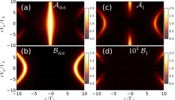
The Majorana LDOS Adot andBdot shown in Figs. 2(a)
and 2(b), respectively, as functions of ε and eVg [same
FIG. 2. (Color online) Color map of the local density of states for Majoranas “A” (top) and “B” (bottom) at the dot (left) and at the first site of the chain (right) as a function ofεandeVgfort= 10 meV, =0.2t, ŴL=40μeV, t0=10ŴL, andμ=0. Panel (d) shows 104B
FIG. 3. (Color online) ConductanceGas a function ofμfort= 10 meV, =0.2 meV, and (a)t0=10ŴL and different values of εdotand (b)εdot=0 and distinctt0’s. The lighter (yellow) and darker
(green) regions in (a) and (b) highlight the topological (|μ|< t) and trivial (|μ|> t) phases of the chain, respectively. Panels (c) and (d) correspond to (a) and (b), respectively, but for=0.
parameters as in Fig.1(f)], display a zero-energy peak inAdot
and none in Bdot. This shows that the pinned dot-Majorana
peak in Fig.1(f) arises from the Majorana A only. We note that the peaks inBdotatε≈ ±7ŴL(foreVg =0) are affected
by the dot-wire Majorana coupling as compared to the=t
case. For couplings to any ordinary fermionic wire modes, the dot LDOS would obey Adot=Bdot, and it would split and
would broaden.
Figures2(c)and2(d)show that the Majorana LDOS of the first chain site A1 andB1 have no zero-energy peaks, thus,
indicating that the wire end mode has, indeed, leaked into the dot. We see two peaks in A1 at ε= ±7ŴL [see Fig. 2(b)]
resulting from the coupling ∼t0 between A1 and Bdot; see Fig.1(a). A careful look at Fig.2(c)reveals an enhancement of the zero-energy peaks for eVg 5ŴL as a result of the
coupling between the dot Majorana A and the Majoranas of the chain via a finiteεdot. The strength of this peak is much smaller than its magnitude without the dot.
Figure 3(a) shows the conductance G vs μ for several
εdot’s [same parameters as in Figs.1(f)and1(g)]. Forεdot=0 [circles (black)] and |μ|> t (trivial phase), G arises from the single-particle dot level atεF. The effect of the chain is
essentially to shift and broaden εdot so that the value e2/ h is reached only for|μ| ≫t. Asμvaries across±t, the wire undergoes a trivial-to-topological transition, andGsuddenly decreases toe2/2has the leaked dot Majorana appears. For
εdot=0, the asymptotic (|μ| ≫t) value ofG is no longer
e2/ hasεdotcannot attainεF. The squares (red) and diamonds
(blue) in Fig.3(a)show a tiny conductance forμ > t. However, as|μ|becomes smaller thant, both curves rapidly go toe2/2h. In Fig. 3(b), we fix εdot=0 and plot the conductance
G as a function of μ for distinct t0’s. As t0 increases, G remains pinned ate2/2hin the topological regime, whereas, it decreases in the trivial phase since the dot level shifts due to the chain self-energy∼t2
0. Figures3(c)and3(d)showGfor=0 and the same parameters as in Figs.3(a)and3(b), respectively. For|μ|< t,Gis very sensitive toεdot for a fixedt0=10ŴL
[Fig.3(c)] and tot0 forεdot=0 [Fig.3(d)], which contrasts with its practically constant value for =0.2t, Figs. 3(a) and3(b). This is so because the wire acts as a third normal lead for=0 andt0=0, so the source drainG, e.g., forμ=0, reduces toG=(e2/ h)Ŵ
L/(ŴL+Ŵchain), whereŴchain=2t02/t is the broadening due to the chain [31]. Curiously, fort0 = 11.18ŴL andεdot =0, theGcurves are indistinguishable for
=0 and=0, being pinned ate2/2hin the topologicaland trivial phases, cf. squares in Figs.3(d)and3(c). Therefore, the peak valueG=e2/2h, first found in Ref. [27] in a similar setup as ours but only for an on-resonance dot (i.e.,εdot=0=εF),is
not per sea “smoking-gun” evidence for a Majorana end mode in conductance measurements as we find that this peak value can appear even in the trivial phase of the wire. One should vary, e.g.,εdot and/ort0 to tell these phases apart as we do in Fig.3. Finally, the kinks in Fig.3(d) [e.g., diamonds (blue) and stars (green)] result from discontinuities inchain[31] at
μ= ±t.
V. CONCLUDING REMARKS
We have used an exact recursive Green’s-function approach to calculate the LDOS and the two-terminal conductance
G through a quantum dot side coupled to a Kitaev wire. Interestingly, we found that the end Majorana mode of the wire leaks into the quantum dot, thus, originating a resonance pinned to the Fermi level of the leadsεF. In contrast to the usual
Kondo resonance arising only forεdot belowεF, this unique
dot-Majorana resonance appears pinned toεF even when the
gate-controlled energy level εdot(Vg) is far above or below
εF, provided that the wire is in its topological phase. This
leaked Majorana dot mode provides a clear-cut way to probe the Majorana mode of the wire via conductance measurements through the dot.
ACKNOWLEDGMENTS
We acknowledge helpful discussions with F. M. Souza. J.C.E. also acknowledges valuable discussions with D. Rainis. This work was supported by the Brazilian agencies CNPq, CAPES, FAPESP, FAPEMIG, and PRP/USP within the Re-search Support Center Initiative (NAP Q-NANO).
[1] D. Goldhaber-Gordon, H. Shtrikman, D. Mahalu, D. Abusch-Magder, U. Meirav, and M. A. Kastner,Nature (London)391,
156(1998).
[2] S. M. Cronenwett, T. H. Oosterkamp, and L. P. Kouwenhoven,
Science281,540(1998).
[3] A. A. Golubov, A. Brinkman, Y. Tanaka, I. I. Mazin, and O. V. Dolgov,Phys. Rev. Lett.103,077003(2009).
[4] R. M. Lutchyn, J. D. Sau, and S. Das Sarma,Phys. Rev. Lett. 105,077001(2010).
[5] Y. Oreg, G. Refael, and F. von Oppen, Phys. Rev. Lett.105,
177002(2010).
[6] A. Y. Kitaev,Ann. Phys.303,2(2003).
[8] V. Mourik, K. Zuo, S. M. Frolov, S. R. Plissard, E. P. A. M. Bakkers, and L. P. Kouwenhoven,Science336,1003(2012). [9] M. T. Deng, C. L. Yu, G. Y. Huang, M. Larsson, P. Caroff, and
H. Q. Xu,Nano Lett.12,6414(2012).
[10] A. Das, Y. Most, Y. Oreg, M. Heiblum, and H. Shtrikman,
Nat. Phys.8,887(2012).
[11] E. J. H. Lee, X. Jiang, R. Aguado, G. Katsaros, C. M. Lieber, and S. De Franceschi,Phys. Rev. Lett.109,186802(2012). [12] A. D. K. Finck, D. J. Van Harlingen, P. K. Mohseni, K. Jung,
and X. Li,Phys. Rev. Lett.110,126406(2013).
[13] K. T. Law, P. A. Lee, and T. K. Ng,Phys. Rev. Lett.103,237001
(2009).
[14] D. I. Pikulin, J. P. Dahlhaus, M. Wimmer, H. Schomerus, and C. W. J. Beenakker,New J. Phys.14,125011(2012).
[15] H. O. H. Churchill, V. Fatemi, K. Grove-Rasmussen, M. T. Deng, P. Caroff, H. Q. Xu, and C. M. Marcus,Phys. Rev. B87,241401
(2013).
[16] M. Franz,Nat. Nanotechnol.8,149(2013).
[17] Interestingly, J. Klinovaja and D. Loss, Phys. Rev. B 86,
085408(2012) have reported Majorana modes leaking across a superconducting-normal interface. See also D. Chevallier, D. Sticlet, P. Simon, and C. Bena,ibid.85,235307(2012). [18] A. C. Hewson, in The Kondo Problem to Heavy Fermions,
edited by D. Edwards and D. Melville, Cambridge Studies in Magnetism (Cambridge University Press, Cambridge, UK, 1993).
[19] When the Kondo resonance coexists with the dot-Majorana mode, the total conductance through the dot should ideally attain 3e2/2h[e2/ h(due to Kondo)
+e2/2h(Majorana)] as was found
by M. Lee, J. S. Lim, and R. L´opez,Phys. Rev. B87,241402
(2013) for a dot in the resonant-tunneling regime. See also Cheng et al., arXiv:1308.4156 and A. Golub, I. Kuzmenko, and Y. Avishai,Phys. Rev. Lett.107,176802(2011) for a discussion on the interplay between Kondo- and Majorana-induced couplings in a quantum dot.
[20] A. Y. Kitaev,Phys.-Usp.44,131(2001).
[21] For an interesting proposal for the realization of the Kitaev chain, see I. C. Fulga, A. Haim, A. R. Akhmerov, and Y. Oreg,New J. Phys.15,045020(2013).
[22] We have also implemented a spin-full version of our system, considering a tight-binding nanowire + Rashba spin-orbit interaction+proximity-induced superconductivity+a Zeeman field (a wire with these ingredients can be mapped onto the Kitaev chain [24,25]), which corroborates our findings. In addition, we have considered a HubbardUterm in the dot and have verified that our results still hold, provided that only a single spin-split dot level lies below the Fermi level of the leads (i.e., Coulomb blockade is irrelevant in this regime). These results will be described elsewhere.
[23] Interestingly, this regime (empty or singly occupied dot) should, by itself, prevent the Kondo effect and Andreev bound states in our setup. Andreev bound states, however, have a strong gate voltage dependence as reported by R. S. Deacon, Y. Tanaka, A. Oiwa, R. Sakano, K. Yoshida, K. Shibata, K. Hirakawa, and S. Tarucha,Phys. Rev. Lett. 104, 076805 (2010) and appear (mostly) as doublets not pinned toεF [see also E. J. H. Lee et al.,Nat. Nanotechnol.9,79(2014)].
[24] J. Alicea,Phys. Rev. B81,125318(2010).
[25] J. Alicea, Y. Oreg, G. Refael, F. von Oppen, and M. P. A. Fisher,
Nat. Phys.7,412(2011).
[26] D. Rainis, L. Trifunovic, J. Klinovaja, and D. Loss,Phys. Rev. B87,024515(2013).
[27] D. E. Liu and H. U. Baranger,Phys. Rev. B84,201308(2011). [28] M. Leijnse and K. Flensberg,Phys. Rev. B84,140501(2011). [29] J. Alicea,Rep. Prog. Phys.75,076501(2012).
[30] E. Prada, P. San-Jose, and R. Aguado, Phys. Rev. B 86,
180503(R)(2012).
[31] The general expression for the conductance at T =0 is G=ŴL(ŴL−Imchain)/[(Rechain)2+(ŴL−Imchain)2]
withchain=2t02(1−
1−g2