A unit root test based on partially adaptive estimation

.

.

.

.

' '

"

FUNDAÇÃD

GE11JUO VARGAS

,~

FGV

EPGE

_ . . .

_._.,

SEMINÁRIOS DE PESQUISA

ECONÔMICA DA EPGE

A unit root test based on partially

adaptive estimation

LUIZ RENATO LIMA

(EPGElFGV)

Data: 11/09/2003 (Quinta-feira)

Horário: 16h

Local:

Praia de Botafogo, 190 - 11

0

_andar

Auditório nO

2

Coordenação:

;

.'

"

A Unit Root Test Based on Partially Adaptive

Estimation.

Zhijie Xiao*

University of nlinois at Urbana-Champaign

Luiz Renato Lima

Getulio Vargas Foundation

September 5,2003

Abstract

This paper constructs a unit root test baseei on partially adaptive estimation, which is shown to be robust against non-Gaussian innovations. We show that the limiting distribution of the t-statistic is a convex combination of standard normal and DF distribution. Convergence to the DF distribution is obtaineel when the innovations are Gaussian, implying that the traditional ADF test is a special case of the proposed testo Monte Carlo Experiments indicate that, if innovation has heavy tail distribution or are contaminated by outliers, then the proposed test is more powerful than the traditional ADF testo Nominal interest rates (different maturities) are shown to be stationary according to the robust test but not stationary according to the non-robust ADF testo This result seems to suggest that the failure of rejecting the null of unit root in nominal interest rate may be due to the use of estimation and hypothesis testing procedures that do not consider the absence of Gaussianity in the data.Our results validate practical restrictions on the behavior of the nominal interest rate imposed by CCAPM, optimal monetary policy and option pricing models.

1 Introduction

In the past decade, econometricians have focused a great deal of attention on the de-velopment of estimation and hypothesis testing procedures in autoregressive time series modela where the largest root is unity. Most of these procedures are based on least square methods in linear regression models and have likelihood interpretations when the data are Gaussian. In the absence of Gaussianity, these methods are less efficient than meth-ods that exploit the distributional information. Indeed, Monte Carlo evidence indicates that the least square estimator can be very sensitive to certain type of outliers and that inference procedures based on least squares estimation may have poor performance (see, e.g., Lucas, 1994).

There is a large literature on nonstationary time series regression with nonnormal in-novations: Cox and Llatas (1991), Knight (1991), Phillips (1995), Lucas (1995), Rothen-berg and Stock (1997), and Juhl (1999), among others. In particular, Phillips (1995) studies robust cointegration regressions and develops fully modified least absolute devi-ations (LAD) and M-estimators for cointegrating regressions. Lucas (1995) considered unit root tests based on M-estimators. Cox and Liatas (1991) and Rothenberg and Stock

(1997) studied robust estimation and inference for nearly integrated autoregressive

mod-eIs without deterministic trend. While these papers focus on the estimation or inference of the autoregression coefficient, the present paper considers the joint estimation of deter-ministic components and autoregressive coefficients, and proposes a unit root test based on partially adaptive estimation method (BickeI1982, pp664; Postcher and Prucha 1986). We consider ADF type of regression with non-normal innovations and show that the lim-iting distribution of the t-statistic tp is a convex mixture of the well-known (detrended) Dickey-Fuller (DF) distribution and a standard normal distribution (independent with the DF distribution). In the extreme case of Gaussian innovations, we recover the famous result that tp converges to the DF limiting distribution. In practice, this result suggests that, in the absence of Gaussianity, robust unit root inference should be carried out using critical values that are different from the ones derived from the DF distribution. We tabulate these new critical values and, therefore, the proposed test is ready to be used by the practitioner.

In empirical analysis, many applications in economics involve data whose distributions may be heavy-tailed, implying that the current practice of testing for unit root in macro-economic variables using tests based on least squares estimation cannot yield a robust unit root inference. In fact, the lack of robust inference may wrongly invalidate many economicjfinance models that assume stationarity in nominal interest rate. As an exam-pIe, the consumption-based capital asset pricing mode} (CCAPM) imposes restrictions on the order of integration of infiation, growth rate of consumption and nominal interest rate: if inflation and growth rate of consumption are stationary, then nominal interest rate has to be stationary as well. However, as showed in Rose (1988), while traditional ADF test indicates that the first two variables are stationary , it is hard to reject unit root for short term rate of nominal interest, implying that the CCAPM is not supported by the data. Furthermore, optimal monetary policy suggests the existence of a constant long-run nominal interest rate (Friedman, 1969 ). In the presence of unit root, nominal interest rate would be unstable and, therefore, a constant long run nominal rate cannot even be defined. As a final example, we could cite the Black-Scholes model used to price interest rate derivatives. This model assume that nominal interest rate is stationary and have Gaussian distribution. We wiIl show that the US nominal rates of interest present strong evidence of heavy-tailed distribution. We cannot reject unit root in those series by using the non-robust ADF test, but we do reject it when we apply the new testo This result seems to suggest that the failure in rejecting the unit root hypothesis in nominal interest rates using univariate tests may be due to the use of estimation and hypothesis testing methods that do not consider the absence of Gaussianity in the data. If devia-tions from normality are considered, restricdevia-tions on the behavior of the nominal interest rate imposed by CCAPM, optimal monetary policies, and option pricing models can be prompt1y restored.

The paper is organized as follows: The econometric model is discussed in Section 2; Section 3 discusses a partiaIly adaptive estimator and a generalized version of the ADF test is proposed in section 4; Section 5 discusses the relevance of the test an presents an empirical example. Section 6 concludes. Proofs are provided in the Appendix. For notation, we use

=>

to signify weak convergence, L for lag operator,

=

for equality in distribution, := for definitional equality, and [nrJ to signify the integer part of nr.

2

The Econometric Model

We consider regressions of the following form:

or

k

Yt = aYt-l

+

2:

'I/1

j tl.Yt-j

+

êb

j=1

k

tl.Yt = fJYt-l

+

2:

'I/1

j tl.Yt-j

+

êt·

j=1

(1)

where ét ia ao üd sequence. The high persistency in real exchange rates (and many other macroeconomic variables) suggests that the coefficient a ia near unity (or p is cIose to O). To test whether or not the time series contain a unit root, we estimate Oi (or p)

and examine the closeness of the estimate to unity (or zero). Most of the traditional estimation procedures and related unit root tests are based on OLS regressions and have likelihood interpretations when the data are Gaussian. In the absence of Gaussianity, asymptotic results of these procedures generally still hold but these methods are less efficient than methods that exploit the distributional information. Monte Carlo evidence indicates that the least squares estimator can be very sensitive to certain type outliers, and inference procedures based on the least square estimation may have poor performance (see, e.g. Lucas 1994). In empirical analysis, many applications in nonstationary time series involve data like nominal interest rates whose distributions are heavy-tailed. It is therefore importaot to consider estimation and hypothesia testing procedures which are robust to departures from Gaussianity and can be applied to nonstationary time series. The present paper addresses some of these issues.

To take into consideration of deterministic trends, following the convention, we

in-clude deterministic trends as added regressors and study the estimation in the following regressions

or

k

Yt = "(' Xt

+

OiYt-l

+

2:

'1/1 jtl.Yt_j

+

êt,

j=1

k

tl.Yt = !,Xt

+

fJYt-l

+

2:

'I/1

j tl.Yt-j

+

êt·

j=1

where Xt is a deterministic component of known formo

(2)

In the simple case in which êt is üd normally distributed, given observations on Yt,

the maximum likelihood estimators of "( and p are the least squares estimators obtained by minimizing

In the absence of Gaussianity in ut, it is possible to follow the idea of Huber (1964) for

the location problem in order to obtain more robust estimators. In this direction, Relles (1968), Huber (1973) introduced a cIass of so-Called M estimators which generally have good properties over a wide range of distributions.

The M-estimator for ("(, Oi,

{'I/Jj}

;=1) or ("(, p,

{'I/1j}

;=1) in model (1) is defined as the solution of the following extreme problem:

where

Qh,

0:, {1/Jj }

;=1)

=

t

cp (tl.Yt - , ' Xt - PYt-1 -

t

1/Jjtl.Yt-j)

t=j+2 j=l

for some criterion function cp. In the case that cp is the true log density function of ê,

Qh,

0:, {1/Jj }

;=1)

is the log likelihood function and the estimator

(9,p,

{~j}

;=1)

given by (3) is the maximum likelihood estimator. Similar regression models, but without lags, have been studied by Lucas (1995) and Xiao (2001).

Denote

h,p,

{1/Ji};=l)'

=

II;

(X~,Yt-1,tl.Yt-1,··

·,tl.Yt-k)'

=

Zt

then we can write the regression as

tl.Yt = II' Zt

+

êt,

and the M estimator

ê

maximizes

n

Q(II)

=

L

cp (tl.Yt - II' Zt). t=j+2

For asymptotic analysis of the deterministic trend, we assume that there is a stan-dardizing matrix Fn such that F;lX[nr] --+ X(r) as n --+ 00, uniformly in r E [O, lJ, where

X(r) is a vector of limiting trend functions. In the case of a linear trend, Fn

=

diag[l,

nJ

and X(r)

=

(1, r)'. If Xt is a general p-th order polynomial trend, Fn

=

diag[l,

n, .... , nPJ

and X(r)

=

(l,r, ... ,rP ).

Following Lucas (1995) and Xiao (2001), we make the following assumptions on êt and the criterion function cp. These conditions are assumed for the convenience of asymptotic analysis. In practice, even if these conditions do not hold, as long as the data has similar distributional properties as the function cp described, Monte Carlo evidence indicates that the M estimation still have good sampling properties.

Assumption AIThe roots of A(L) = 1-L~=l1/JjV alllie outside the unit circle, and

{Et} are i.i.d. random variables with mean zero and variance (12

<

00.

Assumption A2cp(·) possesses derivatives cp' and cp". [u,cp'(u)J has k-th moments for some k

>

2, E[cp'(ut)J = O, 0< E[cp"(ut)J = p,,,, < 00, and cp" is Lipschitz continuous. Assumption A3€t - Et

=

op(l) uniformly for alI t.

Assumptions AI - A3 are standard conditions in asymptotic analysis of M estimators. These assumptions are needed to establish the weak convergence results. We may also replace the moment condition on cp' (u) by boundness conditions of the derivatives of cp,

because the latter and the moment condition on u imply the corresponding condition on

cp'. Assumption A3 is a consistency requirement as in Knight (1989,1991) and it is not needed if cp' is the derivative of a convex function with a unique minimum. Assumptions similar to A3 are also standard in the development of M estimator asymptotics. It is related to Assumption (b) in Theorem 5.1 of Phillips (1995), Assumption C in Xiao (2001), and the same as the assumption on €t - êt in Theorem 1 Df Lucas (1995).

For convenience of asymptotic analysis, we denote A(L)ut = êt and denote [.] as the greatest lesser integer function. Then under Assumption A, as n goes to 00, n-1j2 L~nr] Ut

I,.

A(I?a2 ia the Iong ruo variance of ut, denoted as lrvar(ut). The Iimiting distribu-tions of

(9,

fi,

{:(fij }

;=)

will also be dependent on the weak limit of the partial sums of

<p'(et). Denoting w~ =var[<p'(et)], and 6 = E[<p"(et)], then n-1_/2

El

nrJ

<p'(et)

=> B",(r)

=

w""W2(r) = BM(w~). In fact, under Assumption AI, the partial sums of the vector

process (Ut, <p'(et)) follow a bivariate invariance principIe (see, e.g., Phillips and DurIauf

(1986, Theorem 2.1, 474-476, and 486-489); Wooldridge and White (1988, Corollary 4.2);

and Hansen 1992):

[nrJ

n-1/2:L(ut,<p'(ét))T => (B.,(r),B",(r))T = BM(O,E) t=1

where

E =

[w~

CT

2""]

CT.,,,,,

w""

is the covariance matrix of the bivariate Brownian motion.

We introduce the standardization matrix: Dn

=

diag{ ..;nFn, n, ..;n, .. " ..;n}, the lim-iting distributions ofthe M estimators

(9,

fi,

{;j;j}~

)'

are given in the following theorem.

3=1

THEOREM 1: Given model (1), under Assumptions AI-A3 and the unit root assumption,

~ {~

}k

the limiting distributions of nonlinear regression estimators II =

(9,

fi, 'I/J j , ) are given

J=1

by

Dn(Íi _ lI) =>

~ (ik~;(r)B.,(r)'dr

~2Xk

) -1 (

f

B.,(r~dB",(r)

).

where , B.,(r) = (X(r)', B.,(r»', 9? = [9?1,' . " 9?k]T is a k-dimensional normal variate that is independent with

f

B,.(r)dB"" (r) , and

[ ,,,(O)

r-,,,(k -1)

~.(O)

1

where ',. (h) is the autocovariance function of Ut. In particular,

[

(n-l/2F~

(9 -,) ]

=>

~

: : ( /

W1 (r)W1 (r)'dr )

-1/

W1(r)dW",,(r).

We are particularly interested in the estimation of p (and inference about p, i.e. testing Ho : p = O). To construct a t-statistic of fi, we estimate the covariance matrix by

where 'I/J

=

<p'. This is a heteroskedasticity consistent type covariance matrix estimator as in White (1980). If we consider the t-ratio statistic of fi

t-

-.-L.

'P - se(fi)

THEOREM 2: Given model (1), under Assumptions AI-A3 and the unit root assumption, the limiting distributions of the t-ratio is given by

tp

=

se~p)

=? ; : (el

1

Wl(r)Wl(r)'dre) -1/2 e'

1

W1(r)dW..,(r) (5)

= ;:

(1

Wx(r)2 dr) -1/2

1

Wx(r)dW..,(r)

where W'X(r)

=

W1(r) - foI W1(s)X'(s)ds

(1;

X(s)X(s)'ds) -1 X(r) is the Hilbert

pro-jection in

L.z[O,

1] of W1(r) onto the space orthogonal to X, and e is a collecting vector,

that is, there is one coordinate equal to one that picks the element corresponding to the asymptotic distribution of

s/'M'

and alI the other coordinates equaI zero.

Notice that

t

p is simply tRe M regression counterpart of the well-known ADF t-ratio

test for a unit root.

The limiting distribution of

t

p is not standard and depend on nuisance parameters

since W1 and W.,., are correlated Brownian motions. However, the limiting distribution of

the t-statistic tI> can be decomposed as a simple combination of two (independent) well-known distributions. In addition, related criticaI values are tabulated in the literature and thus are ready for us to use in applications. Notice that we can decompose

1

Bu (r)dBcp (r)

(see, e.g. Hansen and Phillips (1990) and Phillips (1995» as

1

BudB..,.u

+

)..w'I/J

1

BudBu,

where )..ucp

=

uu.,.,lw~ and B..,.u is a Brownian motion with variance

2 2 2

I

2

u..,.u = Wcp - uwp W_u

and is independent with Bu. Using the above decomposition, the limiting distribution of

tp can then be decomposed into

( )

-1/2 ( ) - 1 / 2

~

1

W x (r)2dr

1

Wx(r)dWcp.l(r)

+

À

1

Wx(r)2dr

1

WXdW1

( )

-1/2

~N(O,l)+)"

1

Wx(r)2dr

J

WXdW1

where

2

2 (T ucp

À =2"2'

w1j;wu

W1(r) and W'i'.l(r) are standard Brownian motions and are independent with each other.

distribution. Recall that a quadratic criterion function is obtained when the errors are Gaussian. This result shows that the traditional Dickey-Fuller test willlose power in the absence of Gaussianity: deviations from normality will make the parameter )..2 to be less than one implying that

t

p wiIl converge to a convex combination of standard normal and DF distribution.

Given a consistent estimate of

>.,

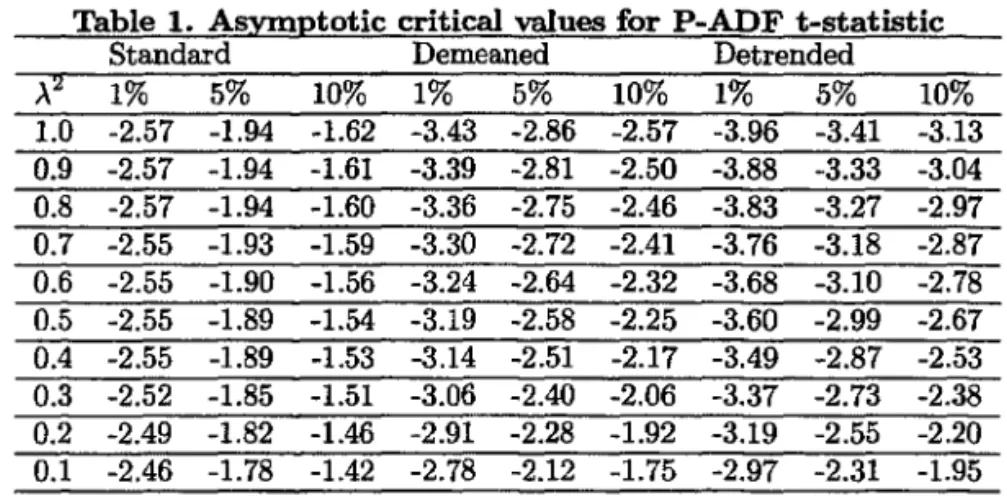
the limiting distribution of tp can be approximated

by a direct simulation. The limiting distribution is the same as that of the covariate-augmented Dickey-Fuller (CADF) test of Hansen (1995). Tables of 1%, 5% and 10% criticai values for the statistic tn(r) are provided by Hansen (1995, page 1155) and re-produced below for convenience. Note that the criticai values are tabulated for values

of

>.2

in steps of 0.1. For intennediate values of

>.2,

Hansen suggest using criticai values

obtained by interpolation.

Table 1. Asvmototic criticaI values for P-ADF t-statistic

Standard Demeaned Detrended

>.'l.

1% 5% 10% 1% 5% 10% 1% 5% 10%

1.0 -2.57 -1.94 -1.62 -3.43 -2.86 -2.57 -3.96 -3.41 -3.13 0.9 -2.57 -1.94 -1.61 -3.39 -2.81 -2.50 -3.88 -3.33 -3.04 0.8 -2.57 -1.94 -1.60 -3.36 -2.75 -2.46 -3.83 -3.27 -2.97 0.7 -2.55 -1.93 -1.59 -3.30 -2.72 -2.41 -3.76 -3.18 -2.87 0.6 -2.55 -1.90 -1.56 -3.24 -2.64 -2.32 -3.68 -3.10 -2.78 0.5 -2.55 -1.89 -1.54 -3.19 -2.58 -2.25 -3.60 -2.99 -2.67 0.4 -2.55 -1.89 -1.53 -3.14 -2.51 -2.17 -3.49 -2.87 -2.53 0.3 -2.52 -1.85 -1.51 -3.06 -2.40 -2.06 -3.37 -2.73 -2.38 0.2 -2.49 -1.82 -1.46 -2.91 -2.28 -1.92 -3.19 -2.55 -2.20 0.1 -2.46 -1.78 -1.42 -2.78 -2.12 -1.75 -2.97 -2.31 -1.95

3

A Partially Adaptive Estimator

The M estimator was motivated by the maximum likelihood estimator. In practice, even if the exact distribution of the innovations is unknown, if the data has similar tail behavior as the density function used in the estimation, then inference based on these method still have good sampling performance. Thus, in applications, we may consider adaptive or partially adaptive estimation methods so that the data density can be approximated.

Althongh from a theoretical point of view , fully adaptive estimation method based on nonparametric estimation (Hansen 1995; Seo 1996; Beelders 1998) is ideal, partia11y adaptive estimation (Bickel 1982, pp664; Postcher and Prucha 1986) may be a practi-cally useful method. In this section, we consider a partialIy adaptive M estimator for (r, p,

{~j}

:=1)'

Taking into account of the weIl documented characteristic of heavy tails in economic and financiaI data, we consider a partially adaptive estimator based on the student-t distributions, although other classes of distributions may be analyzed similarly. The student-t distribution is an important class of distributions (see more discussion in, say, HaU and Joiner 1982) that contains the Cauchy distribution as a special case and the nor-mal distribution as a limit case, and has wide applications in economic analysis. PartialIy adaptive estimator based on this class of distribution is reasonably robusto

{ [

]2}

v+1 n

e

,

k

- - - E

In 1

+ -

6,Yt - , Xt - PYt-l -

L

'If1j6,Yt-j

2 t=j+2 V j=1

where the parameter

e

measures the spread of the disturbance distribution and v is the degree of freedom that measures the tail thickness. Large values of v corresponds to thin tails in distribution. For given parameters

v

and

e,

denoting

e/v

as 9, the 1vfLE of

(T, p, {'If1j}

:=1)

is the solution of the following optimization problem

[-:r,p,

{~j}k_

]

=

argmin

t

In {I

+

9 [6,Yt -1Xt - PYt-l -

t

'If1j6,Yt_j

]2} .

J-l t=J+2 j=l

which allows for the following closed-form solution

fi

n+

[.!:.

tZHWt-29W;l~)Zt]-I.!:.

t Z;Wtlt

n t=1 n t=lt

(6)

where

Wt = (1

+

ffl~)-1 and lt = 6,Yt - Ztfi

Note that

fi

is the least squares estimator of TI and 8

=

~ is the adaptation parameter of the t-distribution

In practical analysis, the parameters v and

e

are not known and has to be estimated. We consider a two-step partially adaptive estimator of (T, p, {'If1j}

;=1)

in which the first step involves a preliminary estimation of the parameters v and

e

(and thus 8). We then replace 8 in 6 by its estimator and perform a second step estimation for (T, p, {'If1j} :=1). In the presence of general disturbance distributions, vand

e

lose their original meaning. However, in the cases where O ::;

v

and O ::;

ê,

v

and

ê

still can be interpreted as estimators of measures of the tailthickness and the spread of the disturbance distribution, and partially adaptive estimator 6 still have good sampling properties.

Potscher and Prucha (1986) discussed the estimation of the adaptation parameters v

and

e.

In particular, if we denote E(IUtlk) as O'k, then for v

>

2, we have

0'2 _ 1f f[v /2]2

O'~

- v - 2 f[(v - 1)/2]2 = p(v) (7)

and

1 vr[(v - 1)/2J2

e

=

1f 0'~f[v/2]2 = q(v, 0'1).

Potscher and Prucha show that p(.) is analytic and monotonically decreasing on (2,00) with p(2+)

=

00 and p(oo)

=

1f/2. Thus, given estimator of 0'1 and 0'2, v can be estimated

by inverting p(v) in 7 and thus an estimator of 9 can be obtained from

Ô = q(v, Ô"1)

=

.!.

r[(v - 1)/2]2

V 1f

Ô"if[v

/2)2

For the estimation of 0'1 and 0'2, we may use the sample moments

A I " ,

I

A Ik

(J"k

= -

~ Ut .

n t

;

4

A Unit Root Test Based on Partially Adaptive Estimation

We propose the following Unit Root Test Based on Partially Adaptive Estimation: 1. Estimate the eriterion Function. Given the time series data, we consider the log-likellhood based on the class of student t distributions: In case of t-distributed innovations, the log-likellhood is given by

n v+ 1 n {

e

2}

L = cons tan t

+

'2

In

e -

-2-t~ ln 1

+

~ [ét]

and estimate the parameters v and

e

as deseribed in the previous Seetion. Denote the estimators as f; and

ê,

we obtain (J.

2. Choosing the foIlowing criterion function

cp(é)

= In {I

+

ê[é]2}

Calculate the M-estimator for

h,

p,

{1/;;} :=1)

in model (1) based on the following extreme problem:

Denote the corresponding t statistic tp.

3. Calculated estimate of

2 2 (7,..'P

À

-- w2_w2

.p u

(8)

and use the estimate of À and the critical v-dlues in Table 1 to test the unit root hypothesis.

5

Monte Carlo Experiments

Monte Carlo experiments were conducted to exalnine the finite sample performance of the P-ADF unit root testo From the construction of the tests, it is apparent that its finite sample performance wiIl depend on sample size, the distribution of the innovations Et,

the bandwidth parameter used to ealeulate the long-run covarianee of {Ut} and {cp'(Et)},

the autoregressive eoeificient a, and the 1(0) persistency of /-Lt. Thus, special attention is paid here to the effects of these elements on the performance of the P-ADF testo Results for the ADF unit root test wiil be reported and compared to the results from the more robust P-ADF testo

In this section, we consider the foilowing modeles)

Yt = ,../ Xt

+

aYt-1

+

/-Lt

/-Lt (3ft-1

+

ét

(9) (10)

where 'Y = O, {ét} is a sequence Df iíd observations drawn from a distribution F. We used two distributions: Gaussian N(O, 1), and student-t with three degrees Df freedom,

We estimated the long-run variance of /-tt as well as the long-run covariance of of {/-tt} and

{cp'(êt)} by using the kernel estimate. For the Kernel function, following Kwiatkowski et alo (1992), we used the Bartlett window 1.

In each replication, we ran the following ADF regression:

llYt

bic

canst.

+

P'Ut-l

+

L

llYt-k + êt

k=l

where the number of lags k was chosen automaticaIly by the Schwartz criterion. (11)

In order to caIculate the P-ADF t-test, we estimated the above regression using one-step M-estimator, which has the closed-form expression given in 6:

Next, we construct the P-ADF t-test based on the one-step M-estimation of 11 and the ADF t-test based on least squares estimation of 11. For the P-ADF t-test, we use covariance matrix 4. For the ADF t-test, we used the traditional covariance matrix

fi

=

;:r2(xtxD-1and ;:r2

=

;:';:/(n -

me -

1).

5.1 Results

Table 1 shows the results for the case where /-tt

=

êt, that is, there is no 1(0) persistence in /-tt. Notice that the bandwidth parameter M corresponds to the number of lags used to caIculate w~ and O"u",(r). Intuitively, for

/3

>

O, the larger

/3

is, the larger !vI need to be in order to estimate ~ and O"u",(r) consistently. In the case that

/3

= O, /-tt is an independent sequence and the long-run variance of /-tt equals the variance of /-tt, implying that we need to set M

=

O. The results presented in Table 1 are within what is predicted by the theory deve10ped in this paper. In particular, when the innovations are drawn from a heavy-tailed distribution, results in Table 1 suggest that: (i) the power of the ADF test declines; (ii) the P-ADF test is much more powerful than the ADF test; (iii) P-ADF test has better size distortion than ADF testo For the case in which the innovations are drawn from a Gaussian distribution, Table 1 shows that both ADF and P-ADF tests have similar power, confirming one more result obtained theoreticaIly.

Table 1. Power and size of 5% test (M

=

O and

/3

= O)

Q 0.85 0.90 0.95 _{0.975 0.99 1}

ADF(t13

»

0.982 0.825 0.284 0.110 0.058 0.047

P-ADF(t(3» 0.997 0.968 0.679 0.322 0.127 0.050

ADF(N(0,1» 0.985 0.827 0.317 0.126 0.066 0.052

P-ADF(N(O,I) ) 0.951 0.764 0.313 0.140 0.071 0.057

Table 2 shows what may happen when one ignores the presence of 1(0) persistence in /-tt in estimating the parameters of w~ and O"u",(r). In other words, the data are now generated with

/3

= 0.7, but the estimation of w~ and O""",(r) ignores this persistence by using M = O. For this case, Table 2 reveals that the P-ADF test will have high size distortion no matter whether the innovations are being drawn from a Gaussian or nonGaussian distribution. The superiority of the P-ADF test over the ADF is maintained when one focus on the power only, but the ADF test has much lower size distortion because its criticaI values do not depend on the estimation of w~ and O"u",(r). Moreover,

lwe estimated fit = Yt - âYt-l, where â =

L.t

Y

' 2 lY' is the least squares estimatar af 0<.

"lt-l

:

DF tests no longer have similar power when innovations are Gaussian, and ADFandP-A

this represents 2 teUs us that therefore, )..2,

a strong contradiction to what is predicted theoretically. In sum, Table

if we ignore the I(O) persistence of I-tt in estimating

w;

and O'u<p(r) and, the P-ADF test willover reject the null of unit root.

Table 2. Power and size of 5% test (M

=

O, and

f3

=

0.7)

a F(t(3» AD P-AD AD P-AD F(t(3» F(N(O,l» F(N(0,1»

0.85 0.90

0.881 0.642

0.988 0.941 0.888 0.650 0.874 0.704

0.95 0.975 0.99 1

0.233 0.105 0.061 0.055

0.704 0.410 0.181 0.087

0.257 0.114 0.064 0.055

0.382 0.199 0.126 0.103

The proble choice of M.

largest integer

m of over rejection of the P-ADF test can be resolved if one uses a correct We propose the sample-dependent choice M

=

[ln(n)], where [xJ is the smaller than or equal to x. This choice is motivated by the fact that ln(n)

.ng function implying that M

=

[ln(n)J

=

op(n), which guarantee that is a slowly varyI

)..2 is consisten eliminate the

tly estimated. Results in Table 3 seems to suggest that this choice does problem of over rejection identified in Table 2.

able 3. Power and size of 5% test (M

=

[ln(n)], and

f3

= 0.7)

a 0.85 0.90 0.95 0.975 0.99 1

AD F(t(3» 0.881 0.642 0.233 0.105 0.061 0.055

P-ADF(t(3» 0.970 0.874 0.541 0.246 0.091 0.041

ADF(N(O,l» 0.878 0.650 0.257 0.114 0.064 0.055

P-ADF(N(O,I» 0.797 0.573 0.248 0.120 0.064 0.052

5.2 Outiers

We next investigate the performance of the ADF and P-ADF tests when innovations are contaminated by outliers. In this section, the model

Yt = 'Y' Xt

+

aYt-l

+

êt (12) is considered. The simulation experiment is set up as follows. First, we set the parameter 'Y =

o.

Next, n normal iid variables êt are generated with mean zero and unit variance. The next step is to construct a new series lt using random numbers Vt uniformly

distributed over the interval [O,lJ. The variable lt equals êt except when Vt

<

0.05, in

which case lt = êt

+

Wt. Here, Wt is a contaminating random variable that is being drawn from a N(0,30).

The results are displayed in Table 4 and they confirm what is predicted theoretically. In particular, we notice that the ADF test has lower power and higher size distortion than the P-ADF testo There seems to be no doubt that the P-ADF test performs much better than the ADF test in cases where the innovations are contaminated by outliers.

1

n=200

ADF 0.057

6

Empirical Analysis

In this section, we will explore some implications of nonstationary nominal interest rate for the economicjfinance literature. For the CCAPM and optimal monetary policy, the hypothesis of stationary nominal interest rate plays a crucial role, whereas for the Black-Scholes model, the hypothesis of stationary coupled with Gaussian distributions are necessary to derive correct c1osed-form formulae of option pricing.

6.1 The consumption-based capital asset pricing modelo

Let us assume that: (i) consumers hold dividend-yielding assets to maximize expected additively separable utility over an infinite hoTizon; (b) the utility function is restricted to be constant relative risk aversion; (iü) no production or goods storage is considerEld.; (iv) consumers face an intertemporal budget constraint in the sense that their asset income must match their expenditures on consumption and assets for future savings. Given these assumptions, the consumer will solve the following problem:

max

Et

[l:~o

f3T

ct'1;

/0+ 1]

,o

<

O,

Xi'T

subject to:

where Et denotes the mathematical expectation conditional on information at time t,

,B is the rate of discount, ct denotes consumption at t, Pit is the ex-dividend price of asset

i at time t, Xit is the share of asset i held at t, and dit is the dividend of asset i held at

t. The first-order Euler equation is given by

Et

~

(

~l

) a ri,t+1]

=

1, (13)

where ri,t+1 is the real return of asset i at time t

+

1 and it is defined as ri,Hl =

(Pi,t+1

+

di,t+l)/Pit. If we take the logarithm of equation 13, then we wiIl obtain the

following testable implication

O (14)

log f3

+

oEt(1og(ct+1/ct)

+

Et(log(ri,t+1»

If the growth rate of consumption is stationary, then Eq 14 suggests that real return must also be stationary. Thus, the CCAPM delivers strong restriction on the dynarnic of consumption growth rate and real interest rate, implying that both variables are supposed to have the same order of integration2_{• As showed by Rose (1988), it is relatively easy} to reject the null hypothesis of unit root in the growth rate of consumption, but it is very hard to do so in real interest rates. This empírical finding constitutes, therefore, a a simple and direct rejection of the CCAPM.

A similar result can be obtained in terms of nominal interest rate. Consider Eq 13 expressed in nominal terms

_ _ _ _ _ _ _ _ _ _ E_t

.l.[f3---,(,-C~l)

a Qt/Qt+1R;,t+1] = 1,

taking the logarithm, we obtain

o

= log

fi

+

aEt(log(ct+t/ct»

+

Et (log(qt!Qt+l» +Et (log(Ri,t+l))

(15)

where qt is the nominal price of goods at time t, Rit is the nominal retum on asset i

at t. Eq 15 indicates that if log(ct+t/ct) and 10g(qt!qt+1) are stationary, then 10g(Ri,t+d

must be stationary as weU. Again, as reported in Rose (1988), although one can easily reject the nuIl hypothesis of unit root for inflation and growth rate of consumption, it is not possible to reject it for nominal interest rate by using tradítional ADF tests. This constitutes, again, a violation of the CCAPM.

In this paper, we will show that the failure of past studies in rejecting the hypothesis of unit root in nominal interest rate was probably due to the use of estimation and inference methods that do not consider the absence of Gaussianity in the data. H deviations from normality are considered, then the restriction imposed by the CCAPM can be restored.

6.2 Optimal Monetary Policy

There has been important discussions about how optimal monetary policy can and should regulate the behavior of the nominal interest rate. According to Friedman (1969), a monetary authority maximizing steady-state welfare would choose a low rate of inflation.

As a result, the long ruo rate of nominal interest would be sufficiently close to zero so that the private and social cost of money holding coincide. Later, Khan et aI (2003) showed that an optimal monetar:r policy would set the nominal interest rate at an average leveI that implies defiation, but it wiU be still positive. In sum, optimal monetary policies -suggest the existence of a constant long run nominal interest rate which can be defined as the difference between the asymptotic real interest rate and the asymptotic rate of inflation.3 _{In the presence of unit root, nominal interest rate would not be stable and,} therefore, we could not define a constant long run nominal rate.

6.3 Option Pricing

In so far, we have paid attention to models where the assumption of stationary nominal interest rate plays a crucial role. In the Black-Scholes type option pricing model, the assumption of stationarity and Gaussian distributions are jointly important to derive closed-form formulae of option pricing. Interest-rate derivatives are weU diversified, it ranges from a simple caU option on yields to a complicated structure involving yield-curve swaps in which yields with different maturities are swapped between counterparties. Other interest-rate derivatives include index-amortization swaps, caps, fioors, and delivery options in Treasury bond future contracts (see, say, James and Webber 2000, for more details).

It is well known that the Black-Scholes model assumes that the empirical returns follow a log-normal distribution upon which most of its results are based. While of great importance and widely used, such theoretical option pricing model does not perform well in practice when the distributions are non-Gaussian. As an example, the Black Scholes model underestimates the prices of away-from-the-money options, meaning that the implied volatilities of options form a convex function, rather than the expected fiat line giving rise to the SCK:alled "volatility smile". As we wiIl show, nominal interest rate is stationary but not Gaussian, which implies that one cannot resort to the Black and

Scholes model to implement efficient pricing of derivatives even under the presence of stationary interest rate. Nevertheless, Borland (2002) derived manageable closed-form solutions for option pricing under the presence of non-Gaussianity and, therefore, it can be used to price derivatives of interest rate given the results on nominal interest rate presented in this paper.

7 Empirical Results

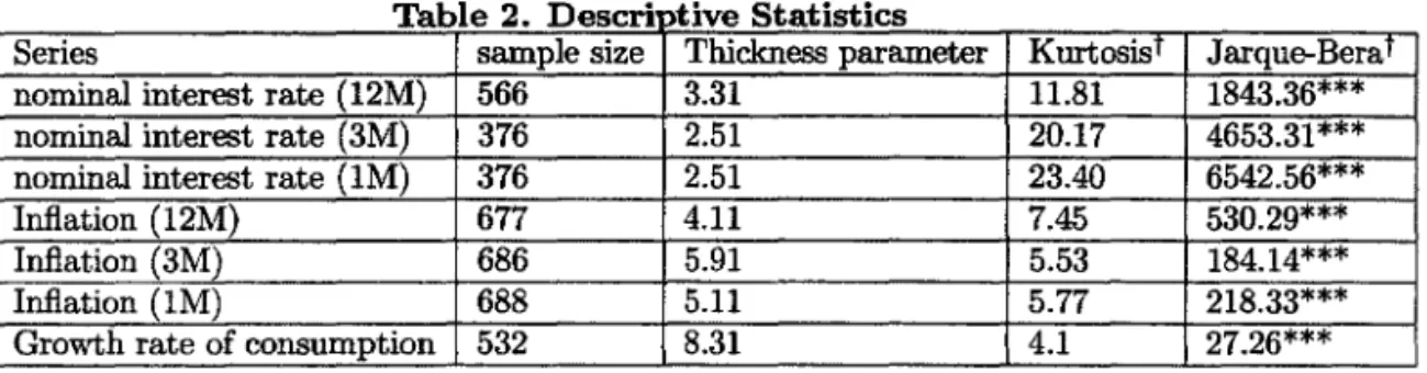
We used monthly data collected from the Federal Reserve Bank of Saint Louis available at http://www.stls.frb.org/fredj. We used l-month and 3-month commercial paper rate for the nominal interest rate with one-month and 3-month maturity. The 12-month treasury bill rate was used for the nominal interest rate with 12-month maturity. Inflation rates were calculated using CPI data- alI urbans and non-seasonally adjusted indexo Data on consumption growth were calculated taking the first difference of the logarithm of personal consumption expenditure. We tried to maximize the sample size going back to the first available observation of each variable. The table below presents some information about our dataset.

Tabl 2 D e eSCM "t" Ive 8t t" t" a I s ICS

Series sample size Thickness parameter KurtosisT _Jarque-BeraT

nominal interest rate (12M) 566 3.31 11.81 1843.36***

nominal interest rate (3M) 376 2.51 20.17 4653.31***

nominal interest rate (1M) 376 2.51 23.40 6542.56***

Inflation (12M) 677 4.11 7.45 530.29***

Inflation (3M) 686 5.91 5.53 184.14***

Inflation (1M) 688 5.11 5.77 218.33***

Growth rate of consumption 532 8.31 4.1 27.26***

t The dah were pre-whitened usiog no interc:ept nnd the number ar lll.gs shown in tnble 3. The symbol (''''''') repast'Dts rejectiun of tht' buli hypotht!tlilS 1I.t. 1% leveI uf tlignificanct!

Table 2 shows two measures of tails. The standard one is the kurtosis. It is well known that whenever this quantity exceeds 3, we say that the data feature excess kurtosis, or that their distribution is leptokurtic, that is, has heavy tails. One can see that, after pre-whitening, alI variables seems to have excess kurtosis, with the series of nominal interest rate presenting the largest ones. Another measure of heavy tail is the thickness parameter of the t-student distribution li, with small values of li corresponding to heavy tails. Again,

we notice that the series of nominal interest rate have very small thickness parameter, suggesting the existence of heavy-tailed distribution for those series.

We next turn to the unit root analysis. We employed the non-robust ADF test and the robust P-ADF testo Results based on the ADF test show that we cannot reject the null hypothesis of unit root for nominal interest rate, but we easily reject it for inflation and growth rate of consumption. This result is qualitatively equal to what is reported in Rose (1988): nominal interest rates are 1(1) whereas inflation and gTOwth rate of consumption are 1(0). Therefore, according to the non-robust ADF test, one could conclude that: (i) restrictions imposed by the CCAPM are false; (ii) a constant long-run nominal interest rate does not exist and, therefore, the behavior of the nominal interest rate is different from what is predicted by optimal monetary policies and; (iii) the black-scholes model is inappropriate to price interest rate derivatives. Results based on the robust P-ADF test confirm that inflation and growth rate of consumption are stationary, but they also show that nominal interest does not have a unit root. In sum, table 3 seems to suggest that the failure of rejecting the null of unit root in nominal interest rate may be due to the

use of estimation and inference methods that ignore the absence of Gaussianity in the data. Since ADF test has low power against nonGaussianity, the stationarity of variables with heavy-tailed distribution, like nominal interest rate, may not be found easily. Our results show that the restrictions imposed by the CCAPM, optimal monetary policy and Black-Scholes model can be promptly restored if one employs the robust P-ADF test4 •

e

.

m o lYSlS

Tabl 3 U ·t Ro t Anal

Variable ADF P-ADF LagsT _{specification}

nominal interest rate (12M) -2.05 -3.01** 6 constant

nominal interest rate (3M) -2.11 -3.67*** 5 constant

nominal interest rate (1M) -2.02 -3.03** 5 constant

Inflation (12M) -3.49*** -4.70*** 14 constant

Inflation (3M) -3.60*** -9.57*** 18 constant

infiation (1M) -5.70*** -6.15*** 8 constant

Consumption (growth rate) -17.45*** -32.33*** 1 constant

t

LA.gs were chosen Bceordihg to the Sc:bw"rtz criterjCtu

Tlu' "lObol ("'."') repruent:'l rejpction Df tb~ Buli hypotbuis at: 1% }t-vpl Df sigDificaDCl'

T~ • • ymboJ (U) upresllots rejectioD Df the bulI hypothub It.t 5% levei ar signi.ficftDCe

8 Conclusion

This paper develops a unit root test based on partially adaptive estimation (P-ADF test), which dclivers power against time series whose innovations are heavy-tailed distributed. ADF type or regression is considered without assuming Gaussian innovations. Under nonGaussian innovations, the t-statistic is shown to converge to a convex combination of normal distribution and Dickey-Fuller distribution. Convergence to the DF distribution is obtained under the presence of Gaussian innovations, which suggest that the ADF test is a particular case of the proposed testo As an empirical example, we show that nominal interest rates are featured with heavy-tailed distribution and that the null of unit root cannot be rejected if one uses the non-robust ADF test, but it is rejected when one uses the robust P-ADF testo Our results suggest that the failure of past studies in rejecting the null hypothesis of unit root in nominal interest rate may be due to the use of estimation and hypothesis testing methods that disconsider the existence of nonnormal distributions in the data. Since financial time series are known to have nonnormal distributions, we encouragc the use of M-estimation techniques on future research involving financial data. Future researchs on M-estimation based tests are also welcome. Important steps on testing stationarity using M-estimation have recently been taken by Koenker and Xiao (2003).

9 APPENDIX

9.0.0.0.1 forro:

Proof of Theorems 1 and 2. We consider regressions of the following

k

ÂYt = '"(' Xt

+

PYt-1

+

L

'l/ljÂYt-j

+

êt,

j=1

4It is true that the Black-Scholes model is still inappropriate to price interest rate derivates because of

where êt is an üd sequence. We may consider an M estimator of (T,a,

{1/Ij};=1)

or

(T,p, {-IPi};=l) that maximizes

Q(T,a,{1/IJ;=1) = tcp (AYt -"('Xt -PYt-1- E1/IiAYt-j)

t=2 i=l

for some criterion function cp. A similar regression, but without lags, has been studied by Lucas (1995).

Denote

(T, p,

{1/1;)

;=1)'

= 9

(x~, Yt-b AYt-b' . " AYt-k)' Zt

then we can write the regression as

and the M estimator

ê

maximizes

n

Q(9) =

L

cp (AYt - ()' Zt) . t=2

For asymptotic analysis of the deterministic trend, we assume that there is a stan-dardizing matrix Fn such that F;lX[nr] -+ X(r) as n -+ 00, uniformly in r E

[0,1],

where

X(r) is a vector of limiting trend functions. In the case of a linear trend, Fn

=

díag[l, n]

and X(r)

=

(1, r)'. If Xt is a general p-th order polynomial trend, Fn

=

díag[l, n, .... , nP]

and X(r) = (1, r, ... , rP ).

The estimators solve the following equation system:

Q(a,"(, {1/Ij};=1)

t

cp (AYt - "('Xt - PYt-1 -

E

1/IiAYt-j)

t=2 j=l

n

t=2

n

FOC:

L

cp' (AYt - (/ Zt ) Zt

=

O

t=l

or let

1/1

= cp',

n

L

1/1 (

AYt - (/ Zt ) Zt

=

O

t=l

Taking a Taylor expansion with respect to êt

=

AYt - (/ Zt around êt = AYt - ()' Zt we

have _{n n}

L

1/1

(êt) Zt -

L

1/1'

(êt) Zt Z

:(8 -

9)

+

RT

=

O

t=l t=l

. We introduce the standardization matríx:

:

under our regularity conditions, (Under the assumptions of Theorem 1)

Dn(ê - 9)

=

[~t/J'

(êt)D:;;1 ZtZ;D:;;l + OP(1)] -1

~t/J

(êt) D:;;l Zt

the following asymptotics hold:

n-2y'f-l

n;/2 tiYt-lYt-l t=l

where

7,(0)

1

By(r)' = (X(r)', By(r»'

Thus,

In particular,

This is a heteroskedasticity consistent type covariance matrix estimator as in White (1980). If we consider the t-ratio statistic of

p

p

t

-P - se(p)

[t. ".

«,)

D;' Z,Z;D;'

r

[t."

«,)'

D;' Z,Z;D;'

1

[t. ,,'

«,)

D;' Z,Z;D;'

r'

~

~

[ J

Bu(r)B., (r)' dr 02Xk]-1

62 Okx2

r

fi-l/2 Dn(Ô - 8) => ~

[ f

B.,(r)B.,(r)'dr

U'if; OkX2

J... [

J

B.,(r)B.,(r)'dr

Ut{> OkX2

fi;.1/2 [

{n-l/2F~;

(9 - 1') ] => : ;

(!

Wl(r)Wl(r)'dr) -1/2

!

W₁(r)dW<p(r).

Thus the t-ratio

t"

=

se~p)

=> : ; (ef

!

W1(r)Wl(r)'dre) -1/2 ef

!

W1(r)dW<p(r)

= ; :

(!

Wx(r)2 dr)

-1/2!

Wx(r)dW<p(r)

where Wx(r)

=

W1(r) - foI W1(S)Xf_(s)ds

(I;

_{X(s)X(s)'ds) -1 X(r) is the Hilbert}

pro-jection in L.2[0, 1] of W1(r) onto the space orthogonal to X.

Notice that

t"

is simply the M regression counterpart of the well-known ADF t-ratio test for a unit root.

The limiting distribution of

t"

is not standard and depend on nuisance parameters since W1 and W.., are correlated Brownian motions. However, the limiting distribution of the t-statistic

tp

can be decomposed as a simple combination of two (independent) well-known distributions. In addition, related criticai values are tabulated in the literature and thus are ready for us to use in applications. Notice that we can decompose

!

Bu (r)dB.., (r)

(see, e.g. Hansen and Phillips (1990) and Phillips (1995» as

!

BudB<p."

+

Àw'if;

!

B.,dB .. ,

where À.,<p

=

uU<Plw~ and B..,.u is a Brownian motion with variance

..

I . .

and is independent with Bu.

1

[I

]-1/2

1

n;.1/2Dn(Ô_(})

=>

W'Ij; Bu (r)Bu (r)'dr Bu(r)dBrp(r)

1 [ / - - , ] -1/2

(I

I )

= wt{J Bu(r)Bu(r) dr BudBrp.u + >'u'lj; BudBu,

=

~~u

[I

Wu(r)Wu(r)'dr] -1/2

I

WudWrp."

>.

[

]

-1/2

+ :;"

I

W,,(r)Wu(r)'dr

I

W"dW"

=

U::~"

[I

W u (r)Wu (r)'dr] -1/2

I

W"dWrp."

+

~:"

[I

Wu(r)W" (r)'dr] -1/2

I

W"dl

( )

2 2 ~2 / ,2 2 2 2 2

Urp... _ Wrp - <TUrp w .. _ WrpW" - U"rp _ 1- uurp

U.I. - w2 - W2w2 - w2w2

'f' '" '" " '" "

The limiting distribution of

tp

ean then be deeomposed into

tp

se~p)

=>

)1-

>.2

(I

Wx(r)2 dr ) -1/2

I

Wx(r)dWrp.1(r)

+ >.

(I

Wx(r)2dr) -1/2

I

_WxdW1

)1-

J..?N(O, 1)

+ >.

(I

Wx(rfdr) -1/2

I

WXdWl

9.0.0.0.2

References

[l]Beelders, O. (1998) Adaptive estimation and unit root tests. Working Paper. Emory

University.

[2]Bickel, P. (1982). On adaptive estimation. Annals of Statistics, 10, 647-671.

[3]Borland, L. (2002). A theory of non-Gaussian option pricing. Quantitative Finance, v. 2, 415-31.

[4]Cheung, Y.W. and K.S. Lai (1997). Bandwidth selection, prewhitening, and the power of the Phillips-Perron testo Econometric Theory 13, 679-691

[5]Cox, D. and Llatas, 1. (1991) Maximum likelihood type estimation for nearly nonsta-tionary autoregressive time series.Annals of Statistics 19, 1109-1128.

[6]Friedman, M. (1969). The Optimum quantity of money. In the Optimum Quantity of M oney, and other Essays, Aldine publishing Company: Chicago.

Grossman, G., Rogoff, K. (eds.), Handbook of International Economics, voL 3,

North-Holland, New York, pp. 1647-1688.

[7] Grenander, U., and M. Rosenblat (1957) Statistical Analysis of Stationary Time Se-ries. New York: John Willey.

[8]James, J. and N. Webber (2000). Interest Rate Modelling. John Wiley & Sons., LTD. [9]Hall, D. and B. Joiner. (1982) Representations of the space of distributions useful in

robust estimation of location. Biometrika, 69, 55-59.

[10] Hansen , B. and S. Lee. (1994) Asymptotic Theory for Garch(l,l) quasi-maximum likelihood estimator. Econometric Theory, 10, 29-52.

[l1]Huber, P.J. (1964) Robust estimation of a location parameter. Annals of Mathematical Statistics, 35, 73-101.

[12]Huber, P.J. (1973) Robust regression: asymptotics, conjectures, and monte carlo.

Annals of Statistics, 1, 799-821.

[13]Koenker, R., and Z. Xiao (2003). Testing stationarity using M-estimation. Working paper, University of lliinois at Urbana-Champaign.

[14JKnight, K. (1991) Limiting Theory for M estimators in an integrated finite variance processo Econometric Theory, 7, 200-212.

[15]Lucas, A. (1994). An outlier robust unit root test with an application to the extended Nelson-Plosser data. Journal of Econometrics 66, 153-174.

[16]Lucas, A. (1995). Unit root tests based on M estimators. Econometric Theory 11, 331-346.

20

lJIUOTECA

MARIO

HENRIQUE SIMONSEW

"

:

;

.

,

[171phillips, P.C.B. (1995). Robust nonstationary regression. Econometric Theory 12, 912-951.

[181phillips, P.C.E. and Z. Xiao (1998). A primer on unit root testing. Joumal of

Eco-nomic Survey 12, 423-469.

[191Potscher, B., I. Prucha. (1986) A class of partially adaptive one-step M estimators for the nonlinear regression model with dependent observations. Joumal of Econometrics 32,219-251

[201Rothenberg, T., and J. Stock (1997) Inference in a nearly integrated autoregressive model with nonormal innovations. Joumal of Econometrics 80, 269-286.

[211Seo, B. Essays on Time Series Econometrics. PhD Disserlation, University of Rochester.

[22]Schmidt, P. and P.C.B. Phil1ips (1992) Testing for a unit root in the presence of deterministic trends. Oxford Bulletin of Economics and Statistics, 54, 257-288. [23]Stock, J.H. (1995) Unit roots, structural breaks, and trends. In R.F. Engle and

Mc-fadden (eds.) , Handbook of Econometrics, volA, pp. 2739-2841. Amsterdam: North-Hoiland.

[24]White, H. and 1. Domowitz (1984). Nonlinear regression with dependent observations.

Econometrica, 52, 143-161.

FUNDAÇÃO GETULIO VARGAS

BIBLIOTECA

ESTE VOLUME DEVE SER DEVOLVIDO A BIBLIOTECA NA ULTIMA DATA MARCADA

N.Cham. P/EPGE SPE L732u

Autor: Lima, Luiz Renato

Título: A unit root test based on partially adaptive estimat

1111111111111111111111111111111111111111

~;3~~48

FGV - BMHS W Pat.:322348/03

000322348

\\\\\\\\\\\\\\\\\\\\\\\\\\\\\\

\\

\\\

.

'.