Temporal aggregation and bandwidth selection in estimating long memory

❊♥s❛✐♦s ❊❝♦♥ô♠✐❝♦s

❊s❝♦❧❛ ❞❡

Pós✲●r❛❞✉❛çã♦

❡♠ ❊❝♦♥♦♠✐❛

❞❛ ❋✉♥❞❛çã♦

●❡t✉❧✐♦ ❱❛r❣❛s

◆◦ ✹✼✽ ■❙❙◆ ✵✶✵✹✲✽✾✶✵

❚❡♠♣♦r❛❧ ❆❣❣r❡❣❛t✐♦♥ ❛♥❞ ❇❛♥❞✇✐❞t❤ ❙❡❧❡❝✲

t✐♦♥ ✐♥ ❊st✐♠❛t✐♥❣ ▲♦♥❣ ▼❡♠♦r②

▲❡♦♥❛r❞♦ ❘♦❝❤❛ ❙♦✉③❛

❖s ❛rt✐❣♦s ♣✉❜❧✐❝❛❞♦s sã♦ ❞❡ ✐♥t❡✐r❛ r❡s♣♦♥s❛❜✐❧✐❞❛❞❡ ❞❡ s❡✉s ❛✉t♦r❡s✳ ❆s

♦♣✐♥✐õ❡s ♥❡❧❡s ❡♠✐t✐❞❛s ♥ã♦ ❡①♣r✐♠❡♠✱ ♥❡❝❡ss❛r✐❛♠❡♥t❡✱ ♦ ♣♦♥t♦ ❞❡ ✈✐st❛ ❞❛

❋✉♥❞❛çã♦ ●❡t✉❧✐♦ ❱❛r❣❛s✳

❊❙❈❖▲❆ ❉❊ PÓ❙✲●❘❆❉❯❆➬➹❖ ❊▼ ❊❈❖◆❖▼■❆ ❉✐r❡t♦r ●❡r❛❧✿ ❘❡♥❛t♦ ❋r❛❣❡❧❧✐ ❈❛r❞♦s♦

❉✐r❡t♦r ❞❡ ❊♥s✐♥♦✿ ▲✉✐s ❍❡♥r✐q✉❡ ❇❡rt♦❧✐♥♦ ❇r❛✐❞♦ ❉✐r❡t♦r ❞❡ P❡sq✉✐s❛✿ ❏♦ã♦ ❱✐❝t♦r ■ss❧❡r

❉✐r❡t♦r ❞❡ P✉❜❧✐❝❛çõ❡s ❈✐❡♥tí✜❝❛s✿ ❘✐❝❛r❞♦ ❞❡ ❖❧✐✈❡✐r❛ ❈❛✈❛❧❝❛♥t✐

❘♦❝❤❛ ❙♦✉③❛✱ ▲❡♦♥❛r❞♦

❚❡♠♣♦r❛❧ ❆❣❣r❡❣❛t✐♦♥ ❛♥❞ ❇❛♥❞✇✐❞t❤ ❙❡❧❡❝t✐♦♥ ✐♥ ❊st✐♠❛t✐♥❣ ▲♦♥❣ ▼❡♠♦r②✴ ▲❡♦♥❛r❞♦ ❘♦❝❤❛ ❙♦✉③❛ ✕ ❘✐♦ ❞❡ ❏❛♥❡✐r♦ ✿ ❋●❱✱❊P●❊✱ ✷✵✶✵

✭❊♥s❛✐♦s ❊❝♦♥ô♠✐❝♦s❀ ✹✼✽✮ ■♥❝❧✉✐ ❜✐❜❧✐♦❣r❛❢✐❛✳

Temporal Aggregation and Bandwidth Selection in Estimating Long Memory

Leonardo R. Souza

EPGE – Fundação Getúlio Vargas

June 2003

Abstract

This paper reinterprets results of Ohanissian et al (2003) to show the asymptotic equivalence of

temporally aggregating series and using less bandwidth in estimating long memory by Geweke

and Porter-Hudak’s (1983) estimator, provided that the same number of periodogram ordinates

is used in both cases. This equivalence is in the sense that their joint distribution is

asymptotically normal with common mean and variance and unity correlation. Furthermore, I

prove that the same applies to the estimator of Robinson (1995). Monte Carlo simulations show

that this asymptotic equivalence is a good approximation in finite samples. Moreover, a real

example with the daily US Dollar/French Franc exchange rate series is provided.

Keywords: Temporal Aggregation, Long Memory, Bandwidth, Spectrum.

JEL classification: C14, C22, C43

1 - Introduction

An important issue on long memory estimation is the level of temporal aggregation to

apply to the time series in order to estimate the memory parameter. Crato and Ray (2002)

explicitly advocate temporal aggregation of long memory time series with added noise in order

to decrease the noise-to-signal ratio, whereas Ohanissian, Russell and Tsay (2003) propose

temporal aggregation to distinguish between true and spurious long memory. Furthermore, while

many authors have used different frequencies to estimate long memory in their empirical

studies1, other lot have studied the theoretical properties of temporally aggregated long memory

processes2. Moreover, Monte Carlo simulations by Souza and Smith (2003) show that temporal

aggregation may reduce the bias caused by short memory components while increasing the

1

Diebold and Rudebusch (1989), Tschernig (1995), Bisaglia and Guégan (1998) and Chambers (1998), to name a few.

2

estimates standard error, the latter conclusion apparently due only to the shortening of the series

imposed by aggregation.

An older issue concerns the spectral bandwidth to use in semiparametric

frequency-domain estimation methods for long memory. It is agreed that the wider bandwidth used, the

lower the estimates standard error. On the other hand, as long memory relates to the low

frequencies of the spectrum, using a larger bandwidth makes the semiparametric estimation

more susceptible to biases due to short memory components (see, for example, Souza and

Smith, 2002, Smith, Taylor and Yadav, 1997).

Reinterpreting results of Ohanissian, Russell and Tsay (2003), I show that,

asymptotically (for fixed aggregation level), aggregating the series to estimate long memory by

Geweke and Porter-Hudak’s (1983) estimator (GPH) is equivalent to reducing the spectral

bandwidth to a specific number (band) of frequencies, such that the same number of frequencies

is used both in the original and in the aggregated series. This equivalence is in the sense that

their joint distribution is asymptotically normal with common mean and variance and unity

correlation. I prove the same equivalence for the Gaussian semiparametric estimator (GSPR) of

Robinson (1995) and conjecture that some kind of equivalence must hold for other

periodogram-based estimators. Monte Carlo simulations show that the correlation between aggregated and

(specific) low bandwidth estimates approaches one very fast for ARFIMA (0,d,0) and ARFIMA

(1,d,0) processes, but considerably slower if a negative moving average component is present. In

addition, the estimates mean and standard error are very similar.

The daily US Dollar/ French Franc exchange rate series from October 20, 1977 to

October 23, 2002 is studied. In a long memory stochastic volatility (Breidt, Crato and Lima,

1998) model framework, the logarithm of the squared returns are analysed and the absence of

long memory is rejected by the Lo’s (1991) modified R/S test. For different levels of

aggregation and same number of frequencies used the variation in estimates is minimal

compared to the same level of aggregation and different number of frequencies.

Section 2 briefly explains long memory processes and the GPH and GSPR estimators, as

well as the asymptotic equivalence. Section 3 shows some numerical results, Section 4 studies

the US Dollar/French Franc exchange rate series and Section 5 offers a final consideration.

Technical details and proofs are relegated to the Appendix.

2 – Long memory processes

Stationary long memory processes are defined by the behaviour of the spectral density

Definition 1: if there exists a positive function cf(λ), λ∈(−π,π], which varies slowly as λ tends to zero, such that d ∈ (0, 0.5) and

0 as )

( ~ )

(λ c_f λ λ−2d λ→

f , (1)

where f(λ) is the spectral density function of the stationary process Xt, then Xt is a stationary

process with long memory with (long-)memory parameter d.

Xt is said to follow an ARFIMA(p,d,q) model if Φ( )(B 1−B X)d t =Θ( )B εt, where εt is a

mean-zero, constant variance white noise process, B is the backward shift operator such that BXt

= Xt-1, and Φ(B)= 1-φ1B-…-φpBp and Θ(B)=1+θ1B+…+θqBq are the short-run autoregressive

and moving-average polynomials, respectively. ARFIMA processes are stationary and display long memory if the roots of Φ(B) are outside the unit circle and d ∈ (0, 0.5).

2.1 – The GPH estimator

The GPH estimator, proposed by Geweke and Porter-Hudak (1983), estimates d from the

spectrum behaviour close to the zero frequency. Taking the log of the both sides of (1) yields

λ λ

λ) log ( ) 2 log (

log f ≈ c_f − d _{in the positive vicinity of the zero frequency. Replacing the}

spectral density function by the periodogram I(λj) and rearranging gives way to:

j j f

j c d

I(λ )=log (λ)−2 logλ +ξ

log , (2)

where λj = 2πj/T, j = 1, …, m, are the Fourier frequencies and T is the sample size.

Least-squares estimation applied to (2) yields an estimate for d. Hurvich, Deo and Brodsky (1998) prove that this estimator is consistent provided that the time series is Gaussian and m → ∞ and

(m log m)/T → 0 as T →∞. They also prove asymptotic normality:

) 24 / , 0 ( )

ˆ

(d d N π2

m − →D . (3)

Note that the variance of the asymptotic distribution depends only on the number of Fourier

frequencies used in the estimation. It is usual to consider m as a function of the series length (m

= F(T)).

2.2 – The Gaussian semiparametric estimator of Robinson (GSPR)

This estimator was proposed by Robinson (1995) and maximises the approximate form

of the frequency domain Gaussian likelihood, where discrete averaging is carried out over a

= =

−

= m

1 j

j m

1 j

j d 2

j log( )

m d 2 I m

1 log ) d (

R λ λ . (4)

Robinson (1995) outlines the conditions under which this estimator is consistent and the ones

under which it is asymptotically Gaussian so that:

) ¼ , 0 ( )

ˆ

(d d N

m − →D . (5)

It is important to point out that (5) is proved without imposing Gaussianity in the series.

Again, the asymptotic variance depends only on the number of periodogram ordinates used in

the estimation, but note that the GSPR has lower asymptotic variance than the GPH if we

consider the same number m of periodogram frequencies used. However, one must bear in mind

that different assumptions are made in proving the results for the two estimators, details of

which are found in the respective papers.

2.3 – Temporal aggregation of long memory processes

If one considers n as the level of temporal aggregation, it is equivalent to observing a

flow variable at a frequency 1/n times the original one. In other words, summing up every n-th

and its preceding n-1 observations. The aggregated variable Yt is observed as follows:

Definition 2: Let Xt be a process observed at times t = 1, …, TX. Then

−

=

−

=

− =

= 1

0

1

0

n

i

n

i

nt i i

nt

t X B X

Y , t = 1, …, Ty ; Ty = TX/n.

Ohanissian, Russell and Tsay (2003) prove that if the series is Gaussian then the GPH

estimators from the original and the aggregated series are asymptotically jointly normal, and the

covariance between them is asymptotically equal to the variance of the estimate from the

original series. Although they consider that less frequencies are used in the estimation of the

aggregated series than in the estimation of the original series (mX > mY), the proof is still valid

and hence the result holds for the cases in which the same number of frequencies is used for

both. In this case (mX = mY), as asymptotically the estimator variance depends only on the

number of frequencies used (see equation (3)), the variances are equal and the correlation

approaches one as T →∞.

To sum up, these estimates are asymptotically unbiased, jointly Gaussian with the same

variance and correlation one. Reinterpreting their results, there is an asymptotic equivalence

method and using a specific lower number of frequencies to estimate the long memory in the

original series, such that the same number of frequencies is used in the original and in the

aggregated series. Consider, for example, the case where m = F(T) = Tα, 0<α<1. Asymptotically, estimating Xt using F(TX) frequencies is equivalent to estimate Yt using F*(TY)

= F(TX) = nαF(TY). Or, alternatively, estimating Xt and Yt both using F(TY) frequencies yields

asymptotically equivalent estimates.

In this paper I prove that the same equivalence applies to the GSPR estimator. However,

it is not assumed Gaussianity in the data as in the GPH. Furthermore, Lemma 1 of Ohanissian et

al. (2003) allows one to conjecture that other semiparametric long memory estimators must have

some kind of asymptotic equivalence. The technical proof and details are found in the

Appendix. The next Section contains simulations that show that even with a small sample size

the estimates from the original and the aggregated series are correlated almost to the unity, both

for the GPH and the GSPR.

3 – Simulations

This Section presents the results of simulations with Gaussian ARFIMA series. The

simulation exercise consists of generating synthetic series of different lengths (TX = 200, 500,

1000) and computing mean, standard deviation and correlations between the estimates from the

original series and aggregates up to aggregation level equal to 6 (n = 2, …, 6) over 500

replications of each model. The number of periodogram ordinates (m) to be used in the

estimation, however, is held fixed across all aggregation levels, even though the number of

observations decreases from TX (original series) to TY,n = TX/n (aggregated series with

aggregation level n). This is equivalent to use a shorter bandwidth in the long memory

estimation of the original series. The idea is to compare the estimation with “reduced

bandwidth” on the original series to the one with “usual bandwidth” on the aggregated series,

illustrating thus in the finite sample the asymptotic equivalence between aggregating the series

and reducing the bandwidth. To be precise, m should vary with TY,n instead of TX (how the

experiment is designed). However, both cases are equivalent once m is the same in estimating Xt

and Yt, and we use for simplicity the original series sample size as the argument of F(T). Doing

so, there is no need to estimate the long memory of Xt for every m = F(TY,n), n = 2, …, 6, but

only for m = F(TX). Given the asymptotic joint Gaussianity, these statistics are sufficient to

The models considered are ARFIMA (0,d,0), ARFIMA (1,d,0) with φ = 0.8, and

ARFIMA (0,d,1) with θ = -0.8, for d = -0.3, -0.1, 0, 0.1, 0.3. Table 1 shows mean and standard deviation of GPH estimates of ARFIMA (0,d,0) aggregates up to n = 6 (the original series is

equivalent to an aggregate with n = 1) and m = TXα, α = 0.4, 0.5 and 0.6, for all the series, where

TX is the length of the original series. The mean and the standard deviation of the estimates must

be compared across lines, as the aggregates are disposed in columns. Note that when TX = 200,

there are not enough periodogram observations to compute the GPH estimates for n = 5, 6 and m

= TX0.6. As to the results, the standard deviation remains almost constant across aggregates and

varies slightly across values of d, this variation probably due to sample variation (which does

not occur across aggregates). In this small sample exercise, the estimates standard deviation is

apparently only determined by m, as in the asymptotic behaviour. However, they are higher than

their asymptotic counterparts, given as follows; 0.227, 0.185 and 0.166 respectively for TX =

200, 500 and 1000 and α = 0.4; 0.171, 0.137 and 0.115 for α = 0.5; and 0.131, 0.100 and 0.081

for α = 0.6. The bias is small but increases slightly as the series is aggregated, increasing the

absolute value of the estimates. The larger the bandwidth used the more marked are the

differences between estimates. Table 2 shows the corresponding results for the GSPR. They are

qualitatively similar to those of the GPH estimator, attaining, however, lower standard deviation

for all processes. The bias is comparable. Moreover, the results are slightly more uniform than

for the GPH, both for the mean and the standard deviation.

It is well known that first-order negative AR and positive MA components do not entail

substantial bias in long memory estimation. The corresponding results are not shown but are

available from the author under request. A positive AR and a negative MA components,

however, bias respectively upward and downward long memory estimation (see, for example,

Souza and Smith (2002) and Smith, Taylor and Yadav (1997)). This is what is observed in Table

3. Table 3 shows the results for the GPH estimates for ARFIMA (1,d,0), φ = 0.8, and ARFIMA

(0,d,1), θ = -0.8, processes, with α = 0.5. The results concerning standard deviation of the

estimates agree with those from Table 1 (α = 0.5), being slightly larger in some cases, especially when the process is an ARFIMA(0,-0.3,1). The bias increases in some cases heavily with

aggregation, particularly when d = -0.3. Using the same number of periodogram ordinates as in

the original series offsets the bias reduction obtained by aggregating series in the presence of

short memory components (see Souza and Smith, 2003), while keeping constant the variance of

the estimates. In general, the MA increases the gap between the average estimates from the

clear, sometimes increasing and other times decreasing it. Table 4 shows the same as Table 3,

but for the GSPR instead of the GPH. The results are qualitatively similar to those from the

GPH and the bias is comparable across all processes. The standard deviation, however, is lower

for the GSPR and varies slightly less across aggregates.

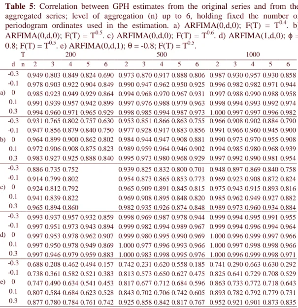
Table 5 shows the correlations between GPH estimates from the original series and the

aggregates up to order 6. The results refer to the same processes and bandwidths considered in

Tables 1 and 3. The correlations are very high, being virtually one in some cases (specially

between the original series and n = 2, positive values of d, highest sample sizes and when an AR

is present). Regarding the results from previous tables and this one, we conclude that in general

the asymptotic equivalence is a good approximation in small samples. The correlation increases

with the series length, as expected, and with d for all processes studied and bandwidths tried.

The increase with d is expected, at least for the GSPR, as the convergence order depends on the

value of this parameter, increasing as d increases (details in the Appendix). On the other hand, it

decreases as the aggregation level n increases. It is noticed that the less bandwidth is used the

closer to unity are the correlations. Remember that in Table 1 the difference between means are

less marked in this case. These results allow us to conclude that the larger the bandwidth used in

the estimation (the higher m) the larger must be T to the asymptotic relationship be a good

approximation to the actual relationship. Furthermore, these results make sense with the theory,

since the order of convergence (of the asymptotic equivalence) is dependent on the number of

periodogram ordinates used in the estimation3. Adding short memory components to the purely

fractionally integrated process affects the results as follows: the AR component seems to

accentuate the correlation, whereas the MA inflicts the inverse consequence. Remember the

effects of these components on the gap between average estimates from the original and the

aggregated series. For small samples, hence, the equivalence is a better approximation when an

AR component is present and is a worse one when there is an MA component, observed the

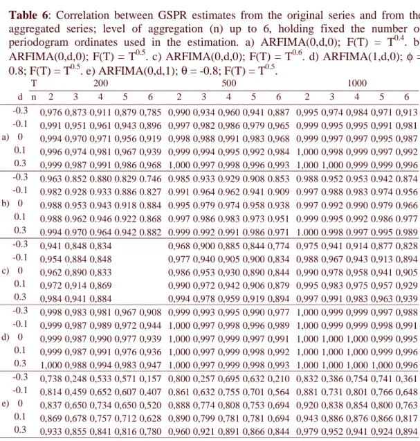
parameter signs and magnitude used. Table 6 shows the same as Table 5, but for the GSPR

estimation method. This method yields correlations consistently higher than those from the

GPH, albeit by a small margin, hinting that the equivalence as an approximation in small

samples is more accurate for the GSPR. The results for the GSPR are consistent with those for

the GPH.

If instead of m = F(TX) one considers m = F(TX/n), which is the usual way to proceed in

practice, the correlations are high but not so close to the unity. For example, for the ARFIMA

3

(0,d,0), the correlation between GPH estimates with n = 1 and n = 2 are around ¾ for all values

of d considered and T = 200; and around 0.8 for all values of d considered and T = 1000. These

correlations, although of interest, are less relevant to the paper results. They are not shown in

tables here but are available from the author under request, as well as the corresponding

correlations not shown here for some combinations of processes and bandwidths.

4 – Real example

This example aims to verify in an actual series what one should expect the proximity

between estimates would be if long memory was estimated from aggregates with different levels

using the same number of periodogram ordinates. For this purpose, the daily US Dollar/ French

Franc (US$/FF) exchange rate series is considered from October 20, 1977 to October 23, 2002

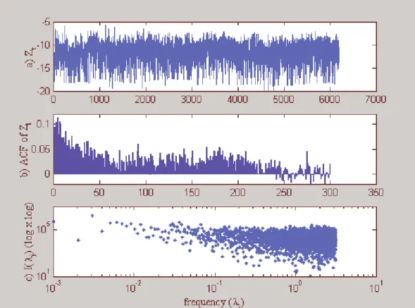
(25 years). More specifically, the natural logarithm of the squared returns is analysed. There are

68 (approximately 1.09%) zero returns existent in the 6264 workdays which were simply

skipped, as well as the holidays. The series, its autocorrelation function (ACF) up to lag 1000

and its periodogram are shown in Figure 1, where the reader can notice the apparent long

memory features such as persistently positive ACF (up to lag 250), and the periodogram

scattered around a frequency power near the frequency zero. The same series is studied in Souza

(2003) and is consistent with the Long Memory Stochastic Volatility (LMSV) model proposed

by Breidt, Crato and Lima (1998), which is givenby the following relation:

t t

t Y

R =σexp( /2)ε , (6)

where Yt is a stationary Gaussian long memory process independent of εt, mean zero iid white

noise, and Rt is the (log-)return. The analysed series is then:

t t t

t R Y v

Z ≡log( 2)=µ+ + , (7)

where µ = (log σ2 + E[log εt2]) and vt = (log ε2 – E[log εt2]) is iid mean zero. Zt is then a

sum of a Gaussian long memory process and a white noise. The kurtosis of the series in study is

approximately 3.68 and the skewness –0.79, so that the Jarque-Bera test rejects the hypothesis of

Gaussianity at 1% confidence level. This does not mean that the Gaussianity of the

non-observable Yt is rejected since it is contaminated by the noise vt in the observed Zt. Furthermore,

the reportedly conservative (Teverovsky et al., 1999) modified R/S test of Lo (1991) rejects the

hypothesis of short memory in Zt at a 0.5% level. Although the series is of stock type,

aggregating it as flow is advocated by Crato and Ray (2002) in order to decrease bias from

Table 7 shows GPH and GSPR estimates of long memory for aggregates from

aggregation levels up to 10 (lines), and different number of periodogram observations used in

the estimation (columns; m = 10, 20, 30, 40, 60, 80, 100, 120, 150). It is apparent that the

variation within column (different levels of aggregation, same m) is minimal compared to the

variation across columns (same aggregation levels, different m’s) and this is more pronounced

for GSPR. This illustrates the asymptotic equivalence between aggregating the series and using

a narrower bandwidth in the original one provided that one holds fixed the number of

periodogram observations to be used in the estimation. In other words, there is no need to

aggregate the series just to diminish the bias, it is enough to use a narrower bandwidth in the

estimation.

5 – Final considerations

There are two related discussions concerning the long memory estimation in time series.

One is about the trade-off implied by aggregating the series before semiparametric estimation

and the other concerns the bandwidth to use in semiparametric frequency-domain estimation

methods. Aggregating, as well as using less bandwidth, is known to reduce the bias induced by

short memory components while increasing the estimates standard error.

This paper shows, based on results from Hurvich et al (1998), Ohanissian et al (2003)

and Robinson (1995), that, for long memory estimation purposes, aggregating is asymptotically

equivalent to use a specific lower bandwidth, holding fixed the aggregation level. This specific

lower bandwidth is such that the same number of periodogram ordinates is used in the original

and the aggregated series. The results are valid for the Geweke and Porter-Hudak (1983) and the

GSPR (Robinson, 1995) estimators, but some kind of equivalence must hold for other

periodogram-based semiparametric long memory estimators. A small simulation is provided to

show that, in addition to the estimates mean and standard deviation being very similar, the

correlation between estimates is close to unity even for small sample sizes. These results,

however, are affected by other factors than the sample size, such as the memory parameter d, the

aggregation level, the presence of a short memory component and the bandwidth used in the

estimation. An additional example with the US$/FF exchange rate series illustrates that

aggregating the series makes little difference when using the same number of periodogram

ordinates in the estimation.

Acknowledgements

References

Bisaglia, L. and Guégan, D. (1998), “A comparison of techniques of estimation in long-memory

processes”, Computational Statistics & Data Analysis, 27, 61-81.

Breidt, F.J., Crato, N. and Lima, P. (1998), “The detection and estimation of long memory in

stochastic volatility”, Journal of Econometrics, 83, 325-348.

Chambers, M. J. (1998), “Long memory and aggregation in macroeconomic time series”,

International Economic Review, 39, 1053-1072.

Crato, N. and Ray, B. K. (2002), “Semi-parametric smoothing estimators for long-memory

processes with noise”, Journal of Statistical Planning and Inference, 105, 283-97.

Diebold, F. X. and Rudebusch, G. D. (1989), "Long memory and persistence in aggregate output",

Journal of Monetary Economics, 24, 189-209.

Geweke, J. and Porter-Hudak, S. (1983), “The estimation and application of long memory time

series models”, Journal of Time Series Analysis, 4, 221-237.

Hosking, J.R.M. (1996), “Asymptotic distributions of the sample mean, autocovariances, and

autocorrelations of long-memory time series”, Journal of Econometrics 73, 261-284.

Hurvich, C. M., Deo, R. and Brodsky, J. (1998), “The mean square error of Geweke and

Porter-Hudak’s estimator of the memory parameter of a long-memory time series”, Journal of

Time Series Analysis, 19, 19-46.

Lo, A.W. (1991), “Long-term memory in stock market prices”, Econometrica, 59, 5, 1279-1313.

Ohanissian, A., Russell, J. and Tsay, R. (2003), “Using temporal aggregation to distinguish

between true and spurious long memory”, working paper, available at

http://gsb-www.uchicago.edu/fac/jeffrey.russell/research/wp.htm.

Robinson, P. M. (1995), “Gaussian semi-parametric estimation of long range dependence”,

Annals of Statistics, 23, 5, 1630-1661.

Smith, J., Taylor, N. and Yadav, S. (1997), “Comparing the Bias and Misspecification in

ARFIMA Models”, Journal of Time Series Analysis, 18, 507-528.

Souza, L.R. (2003), “The aliasing effect, the Fejer kernel and temporally aggregated long

memory processes”, working paper, available at

http://www.fgv.br/epge/home/PisDownload/1086.pdf.

Souza, L. R. and Smith, J. (2002), “Bias in the memory parameter for different sampling rates”,

International Journal of Forecasting, 18, 299-313.

Souza, L. R. and Smith, J. (2003), “Effects of temporal aggregation on estimates and forecasts

of fractionally integrated processes: A Monte Carlo study”, International Journal of

Teles, P., Wei, W. W. S., and Crato, N. (1999), “The use of aggregate series in testing for long

memory”, Bulletin of the International Statistical Institute, 52nd Session Book 3,

341-342.

Teverovsky, V., Taqqu, M.S. and Willinger, W. (1999), “A critical look at Lo’s modified R/S

statistic”, Journal of Statistical Planning and Inference, 80, 211-27.

Tschernig, R. (1995), “Long memory in foreign exchange rates revisited”, Journal of

International Financial Markets, Institutions and Money, 5, 53-78.

Appendix

Proof of the asymptotic joint normality with unity correlation between GSPR

estimates from the original and the aggregated series using the same number of

periodogram ordinates m.

Let IXj and IYj be the periodogram ordinates for the j-th Fourier frequency of the original and the

aggregated series respectively. Lemma 1 of Ohanissian et al (2003) reads as

∞ → →

P X_j asT

Y

j nI

I , provided that: Xt is Gaussian; a condition similar to Definition 1

holds; and the level of aggregation n increases at a slower rate than T. However, their proof

seems to be missing a result, so that I provide a revision on it for n = 2, which is found further in

the Appendix. The revised proof makes an alternative assumption on the long memory of the

series, imposing it in the time-domain rather than in the frequency domain. Furthermore, the

revision can be directly applied to their proof with general level of aggregation n, as long it is

held fixed. This result refers to a convergence in probability, and the revision upon their proof

provided in this paper allows one to reach a convergence speed different than theirs:

) / ( ) /

( 2 _P 12d

X j Y

j nI O j T O j T

I = + + − as T → ∞. (A1)

If j is fixed, the second term on the RHS is O(T-1) and the third is OP(T2d-1), but one must

remember that j varies from 1 to m in the estimation methods, and m is related to T. Thus, one

must consider these terms as O(m2/T) and OP(m/T1-2d), respectively. As to the convergence

speed in the general case, note that if IY_j =2I_jX +O(j2/T)+O_P(j/T1−2d) as T → ∞ for n = 2,

then (A1) holds at least for n = 2k, k = 1, 2, 3, …, easily verified by induction.

This assumption may exclude some values of (m, d) used in the simulation. However, it is still

worthwhile keeping them in the simulation, since only the sufficiency of Assumption 1A,

together with Assumptions A1’ – A4’ of Robinson was proved. Moreover, those values of (m,

d) are kept, if not for other reason, for illustration purposes.

Let also Assumptions A1’ – A4’ of Robinson (1995) hold. Robinson proves (5) so that

) ¼ , 0 ( ) ˆ

(d d N

m − →D _{. Let us consider}

n

dˆ the estimator from the aggregated series using

the same number m of periodogram ordinates as the estimator from the original series dˆ . So, (5)

also holds for dˆ , such that dˆ and _n dˆ have the same asymptotic distribution (and hence the _n

same asymptotic mean and variance). If we prove that dˆ_n →_P dˆ as T → ∞ faster than dˆ→_P d,

then the proof is complete, as in this case am1/2dˆ_n +bm1/2dˆ=(a+b)m1/2dˆ+o_P(1) as T → ∞,

for any constants a, b. That means that any linear combination of dˆ and dˆ is asymptotic _n

normal and they are asymptotically unity correlated. For this, we have to prove that

) ( ˆ

ˆ = + −1/2

m o d

d_{n P} asymptotically. For ease of comparison with Robinson formulas, let H0 = d

+ 1/2; Hˆ =dˆ+1/2; and Hˆ_n =dˆ_n +1/2. For those reading the work of Robinson (1995), please note, however, that n in his notation is equivalent to T in ours and refers to the sample size.

Equation (4.2) of Robinson (1995) states that with probability approaching 1, as T → ∞,

(

)

2 2

0 ) ˆ

~ ( )

(

0 H H

dH H R d dH H dR − +

= , where H~−H₀ ≤ Hˆ −H₀ and R(H) is as defined in (4), but

replacing d by (H – ½). Rewriting this, we have:

2 2 0 0 ) ~ ( ) ( ˆ dH H R d dH H dR H H − =

− . (A2)

Robinson (1995) states further that

= − = m j j m H G H G dH H dR 1 0

1 2 _log

) ( ˆ ) ( ˆ 2 ) ( _λ (A3) and

{

}

= , (A4)

where

(

)

Note that

T j

j π

λ = 2 , so it is O(m/T) as λ→ 0+. Furthermore, λ2_jH−1I_j =O_P(1) as λ→ 0+ if H =

H0 + OP(m-1/2). Hence Gˆ (H) O (log (m/T)) OP(logk(T/m)) k

P

k = = .

Now we consider the estimate Hˆ from the aggregated series Y_n t. Let Gˆk,n(H) and Rn(H) denote

for Yt the equivalent to Gˆ_k(H) and R(H) for the original series Xt, holding m fixed across

aggregates. Note that the Fourier frequencies λYj of Yt are related to the frequencies λj of Xt by λY

j = nλj. Using (1) – that is somewhat similar to, though less formally stated than, Assumption A1’ of Robinson (1995) – and (A1), we have then:

(

)

(

)

(

)

)) / ( ) / ( ( log log )) / ( ) / ( ( log 1 ) ( ˆ 1 2 1 2 2 2 1 1 2 2 1 2 2 2 1 2 2 1 2 2 2 1 2 1 2 , 0 0 = + ∆ + − = − − = − − − + + + = = + + + = = + + = m j k H H P k H H X j H j k j H m j H P X j H j k j H m j H P X j H j H k j n k T m T m O T m T m O I n m n T m O T m O I n m n T m O T m O nI n n m H G λ λ λ λ λ λ (A5)

where ∆H = H – H0. A particularization of (A5) for k = 0, 1, 2, followed by straightforward

calculation, gives:

+ +

= +H P ₊ H_∆H

H H n T m O T m O H G n H

G _{1 2}

2 2 2 1 0 2 ,

0 ( ) ˆ ( )

ˆ _;

{

}

n( ) ˆ ( ) log ˆ ( ) log log

ˆ 2 1 2 2 2 1 0 1 2 ,

1 ; (A6)

{

}

2 ( ) ˆ ( ) 2log ˆ ( ) log ˆ ( ) log log

ˆ

Note that the second term on the right hand side of the equations (A6) dominates the third when

H < ½, and the inverse occurs when H > ½. Adapting (A2) for Hˆ gives: _n

2 2 0 0 ) ~ ( ) ( ˆ dH H R d dH H dR H H n n n − =

− , (A7)

{

}

n = − _{. (A9)}

Remembering that Gˆ (H) O (logk(T/m))

P

k = , further calculation on (A8) and (A9), using (A6),

gives:

+ +

= ( ) + log( / ) log( / )

) ( 0 0 0 2 2 2 1 0

0 _{T m}

T m O m T T m O dH H dR dH H dR H P H H P

n _(A10)

and

+ +

= ) + log ( / ) _{+ −} log ( / )

~ ( ) ~ ( ₂ ) ~ ( 2 1 ~ 2 2 ~ 2 ~ 2 1 2 2 2 2 0 m T T m O m T T m O dH H R d dH H R d H H H P H H P n

. (A11)

Equations (4.10) and (4.11) of Robinson (1995) and extensions show that ( 0) = ( −1/2)

m O dH H dR P

and ) (1)

~ ( 2 2 P O dH H R d

= . So the only additional requirement (to A1’–A4’ of Robinson(1995)) to

n

Hˆ converge to Hˆ faster than Hˆ to H0 is that

(

)

2 2 2 1 ) / log( 0 0 0 − + =

+ T m om

T m T m H H H

. This is

satisfied by the Assumption 1A. The proof is complete.

Proof of (A1) with n = 2

This proof is a revision on a specific case of Lemma 1 of Ohanissian et al. (2003). This revision,

however, is directly applicable to a more general case, where n > 2 but is held fixed. The proof

will require an alternative assumption (1B), which is given below. Also, the Proposition 1B is

provided below in order to make the proof simpler. Note that j is to be considered as O(m), since

j = 1, …, m.

Assumption 1B: Xt is stationary and there exists a real number d < 0.5 and a positive function

c k_ρ( ) which varies slowly as k tends to infinity, such that ρ_X(k)~c_ρ(k)k2d−1ask→∞, where

ρX(k) is the k-th order autocorrelation of Xt.

Proposition 1B: ± = +

2 1 1 1 2 2 2 2 2 cos ) 2 ( 2 cos T jx O t T j sin T jx t T j x t T

j π π π

Proof: Proposition 1B is easily verified by expanding cos 2 (2t₁±x)

T j

π

by a Taylor series

around cos 2 (2t₁)

T j

π

. CQD.

Take the periodogram of Xt at the j-th Fourier frequency:

− + = = = + = T t T t t t t T t t X

j t t

T j X X X T I 1 1 1 2 1 2

1 2 1

2

1 ( )

2 cos 2 2 1 π π (B1)

Let n = 2. Then the periodogram of Yt at the j-th Fourier frequency, as a function of Xt, is as

follows: − + + + + = − = = + − − = − = 1 2 / 1 2 / 1 1 2 1 2 2 1 2 2 2 / 1 1 2 2 1 2

1 2 1

2 2 1

1 ( )

4 cos ) )( ( 2 1 T t T t t t t t t T t t t T t t Y

j t t

T j X X X X X X X T I π

π (B2)

After some manipulation on (B1) and (B2), it is shown that IjX and IjY relate to each other as

follows: IY_j =2IX_j +Α+Β, where

− = Α = − 2 / 1 1 2 2 2 cos 1 2 T t t t T j X X T π

π _{and (B3)}

− = − = + − − + + − + + − − =

Β /2 1

1 2 / 1 1 1 2 2 1 2 1 1 1 2 2 2 1 1 2 1 2 2 1 2 2 ) 1 2 ( 2 cos ) 2 ( 2 cos ) 1 2 ( 2 cos ) 2 ( 2 cos 2 T t t T t t t t t t t t T j t T j X X t T j t T j X X

T π π

π π

π . (B4)

Α is OP((j/T)2), since

= − + − − = − 2 4 2 2 ! 4 1 2 ! 2 1 1 1 2 cos 1 T j O T j T j T

j π π

π

.

The revision upon their proof actually occurs from now forth. In order to match the lag between

variables being multiplied in Β, one can take the first term relating to t1=1 and the second term

Ε + − − − + − = Β = − + − − = − 1 1 2 2 1 2 1 2 / 1 1 2 2 2 2 2 2 2

2 ( 1)

2 cos ) 2 ( 2 cos 2 cos 4 cos 2 t T t t T t t t T T j T T j X X T j T j X X T π π π π π

where −

= − = + − + + + − + + + − + =

Ε /2 2

1 2 / 1 1 1 2 2 1 2 1 1 1 2 2 2 1 1 2 1 2 2 1 2 2 ) 1 2 ( 2 cos ) 2 ( 2 cos ) 1 2 ( 2 cos ) 2 2 ( 2 cos 2 T t t T t t t t t t t t T j t T j X X t T j t T j X X

T π π

π π

π _{. (B5)}

Using Proposition 1B, it is straightforward to verify that cos(4πj/T) – cos(2πj/T) and

cos[(T-2)2πj/T] – cos[(T-1)2πj/T] are both O(j/T). Thus, Β = OP(j/T) + OP(j/T2) + Ε.

Now note that

∞ → + = − + − +

+ ~ ( ) asT

2 2 1

1 2 2 / 1 2 2 2 1 1 2 1 2 2 d P X t t T t t t

t X O n

X

T γ and

∞ → + = − + − +

− ~ ( ) asT

2 2 1

1 2 2 / 2 2 1 2 1 1 2 1 2 2 d P X t t T t t t

t X O n

X

T γ ,

where γ~ =γX +µ2

k X

k ; µ being the unconditional mean of Xt (details in Hosking, 1996, p.266),

since Assumption 1B holds (a sufficient condition). Hence, and using Proposition 1B and (B5),

Ε can be written as:

− = ₋ + − + + + + + + + + − + =

Ε /2 2

1 2 2 1 1 2 1 2 2 2 1 1 2 1 2 1 1 1 ) 1 2 ( 2 2 )) ( ~ ( ) 1 2 ( 2 2 )) ( ~ ( T t _d P X t d P X t T j O t T j sin T j T O T j O t T j sin T j T O π π γ π π γ π (B6)

Cancelling terms, we have from (B6)

− = ₋ − + + + + + + − + =

Ε /2 2

1 2 2 1 1 2 2 2 1 1 2 2 1 ) 1 2 ( 2 2 ) ( ) 1 2 ( 2 2 ) ( T t d P d P T j O t T j sin T j T O T j O t T j sin T j T O T j O π π π π π (B7)

Hence Ε= + P ₋ d + P ₋ d = + P _{− d}

T j O T j O T j O T j O T j

O _{1 2}

2 2 1 2 2 2 2

and (A1) holds for n = 2

and, by induction, for n = 2k, where k is an integer greater than zero (the proof for k = 0 is

Table 1: Mean and standard deviation of GPH estimates from various levels of aggregation, holding fixed the number of periodogram ordinates for ARFIMA(0,d,0). G(T) = Tα, α = 0.4, 0.5 and 0.6.

T 200 500 1000

d \ n 1 2 3 4 5 6 1 2 3 4 5 6 1 2 3 4 5 6

α = 0.4 -0.3 -0.274 -0.291 -0.285 -0.312 -0.323 -0.333 -0.299 -0.304 -0.305 -0.317 -0.322 -0.326 -0.289 -0.289 -0.294 -0.296 -0.305 -0.299 (0,d,0) (0.340) (0.335) (0.329) (0.350) (0.357) (0.352) (0.244) (0.243) (0.253) (0.251) (0.256) (0.252) (0.220) (0.219) (0.232) (0.225) (0.215) (0.224)

-0.1 -0.108 -0.111 -0.104 -0.111 -0.129 -0.132 -0.088 -0.089 -0.088 -0.093 -0.092 -0.095 -0.096 -0.098 -0.094 -0.098 -0.095 -0.093 (0.368) (0.366) (0.369) (0.374) (0.386) (0.373) (0.263) (0.263) (0.268) (0.267) (0.265) (0.261) (0.211) (0.212) (0.217) (0.212) (0.210) (0.222) 0 0.004 0.001 -0.001 0.006 0.003 -0.002 -0.005 -0.006 -0.006 -0.002 -0.001 -0.007 0.008 0.008 0.007 0.008 0.007 0.004

(0.344) (0.341) (0.345) (0.345) (0.353) (0.367) (0.236) (0.237) (0.238) (0.245) (0.237) (0.243) (0.217) (0.218) (0.218) (0.215) (0.215) (0.221) 0.1 0.088 0.090 0.095 0.092 0.095 0.104 0.107 0.107 0.111 0.110 0.114 0.111 0.109 0.110 0.110 0.111 0.110 0.113

(0.334) (0.332) (0.342) (0.335) (0.356) (0.353) (0.270) (0.269) (0.272) (0.271) (0.276) (0.272) (0.221) (0.221) (0.222) (0.221) (0.223) (0.229) 0.3 0.319 0.323 0.331 0.339 0.341 0.354 0.307 0.309 0.311 0.313 0.318 0.323 0.318 0.318 0.319 0.321 0.320 0.324

(0.362) (0.360) (0.362) (0.374) (0.369) (0.369) (0.251) (0.250) (0.245) (0.252) (0.253) (0.252) (0.229) (0.229) (0.230) (0.230) (0.230) (0.234) α = 0.5 -0.3 -0.275 -0.290 -0.310 -0.326 -0.346 -0.358 -0.299 -0.305 -0.323 -0.334 -0.339 -0.359 -0.290 -0.295 -0.304 -0.308 -0.322 -0.328

(0,d,0) (0.227) (0.232) (0.230) (0.245) (0.246) (0.259) (0.174) (0.174) (0.180) (0.175) (0.182) (0.189) (0.131) (0.132) (0.131) (0.133) (0.135) (0.134) -0.1 -0.101 -0.102 -0.107 -0.124 -0.134 -0.127 -0.111 -0.114 -0.119 -0.116 -0.122 -0.121 -0.095 -0.097 -0.099 -0.104 -0.102 -0.106

(0.241) (0.242) (0.256) (0.247) (0.249) (0.271) (0.161) (0.161) (0.165) (0.164) (0.170) (0.168) (0.140) (0.140) (0.143) (0.140) (0.141) (0.141) 0 0.001 -0.001 -0.003 -0.001 0.000 -0.003 0.001 0.001 0.000 0.002 0.000 0.004 0.012 0.013 0.013 0.011 0.009 0.014

(0.240) (0.238) (0.244) (0.244) (0.248) (0.271) (0.163) (0.165) (0.165) (0.170) (0.170) (0.172) (0.137) (0.137) (0.132) (0.137) (0.136) (0.135) 0.1 0.101 0.103 0.114 0.116 0.119 0.134 0.094 0.095 0.095 0.099 0.101 0.106 0.095 0.097 0.097 0.099 0.097 0.103

(0.227) (0.223) (0.223) (0.237) (0.238) (0.243) (0.179) (0.178) (0.180) (0.181) (0.182) (0.185) (0.141) (0.141) (0.142) (0.139) (0.144) (0.146) 0.3 0.314 0.323 0.331 0.351 0.365 0.389 0.299 0.303 0.311 0.314 0.324 0.335 0.295 0.296 0.297 0.302 0.304 0.311

(0.225) (0.224) (0.235) (0.232) (0.239) (0.252) (0.167) (0.167) (0.167) (0.171) (0.169) (0.169) (0.133) (0.133) (0.133) (0.133) (0.134) (0.133) α = 0.6 -0.3 -0.272 -0.296 -0.326 -0.343 -0.296 -0.304 -0.335 -0.346 -0.358 -0.379 -0.294 -0.304 -0.317 -0.330 -0.347 -0.360

(0,d,0) (0.169) (0.169) (0.168) (0.190) (0.126) (0.125) (0.128) (0.130) (0.133) (0.136) (0.094) (0.093) (0.094) (0.095) (0.096) (0.101) -0.1 -0.096 -0.102 -0.124 -0.122 -0.085 -0.091 -0.097 -0.103 -0.108 -0.108 -0.107 -0.111 -0.115 -0.118 -0.123 -0.126

(0.153) (0.157) (0.165) (0.180) (0.116) (0.116) (0.118) (0.122) (0.126) (0.127) (0.089) (0.089) (0.088) (0.094) (0.093) (0.096) 0 0.001 0.003 0.009 0.002 0.005 0.004 0.002 0.004 0.005 0.008 -0.003 -0.004 -0.003 -0.006 -0.005 -0.002 (0.155) (0.159) (0.164) (0.177) (0.117) (0.117) (0.120) (0.122) (0.122) (0.127) (0.090) (0.091) (0.093) (0.094) (0.092) (0.094) 0.1 0.102 0.109 0.119 0.129 0.098 0.103 0.103 0.110 0.114 0.121 0.098 0.101 0.103 0.107 0.112 0.117

(0.162) (0.166) (0.177) (0.181) (0.112) (0.116) (0.117) (0.116) (0.117) (0.128) (0.099) (0.099) (0.100) (0.101) (0.101) (0.106) 0.3 0.310 0.329 0.350 0.377 0.312 0.321 0.333 0.349 0.369 0.381 0.300 0.305 0.313 0.323 0.334 0.348

Table 2: Mean and standard deviation of GSPR estimates from various levels of aggregation, holding fixed the number of periodogram ordinates for ARFIMA(0,d,0). G(T) = Tα, α = 0.4, 0.5 and 0.6.

T 200 500 1000

d \ n 1 2 3 4 5 6 1 2 3 4 5 6 1 2 3 4 5 6

α = 0.4 -0.3 -0,311 -0,323 -0,324 -0,345 -0,354 -0,359 -0,322 -0,327 -0,326 -0,340 -0,344 -0,345 -0,313 -0,315 -0,318 -0,320 -0,325 -0,328 (0,d,0) (0,301) (0,304) (0,291) (0,312) (0,312) (0,299) (0,214) (0,214) (0,213) (0,217) (0,221) (0,210) (0,184) (0,182) (0,188) (0,183) (0,180) (0,190) -0.1 -0,133 -0,135 -0,131 -0,139 -0,148 -0,153 -0,123 -0,123 -0,125 -0,125 -0,128 -0,131 -0,114 -0,115 -0,113 -0,117 -0,115 -0,117 (0,326) (0,326) (0,330) (0,322) (0,323) (0,325) (0,232) (0,232) (0,235) (0,233) (0,233) (0,236) (0,185) (0,185) (0,185) (0,184) (0,185) (0,187) 0 -0,027 -0,027 -0,034 -0,027 -0,029 -0,040 -0,031 -0,031 -0,032 -0,029 -0,027 -0,033 -0,021 -0,021 -0,022 -0,021 -0,020 -0,023 (0,298) (0,298) (0,297) (0,290) (0,296) (0,300) (0,207) (0,208) (0,207) (0,210) (0,206) (0,209) (0,183) (0,184) (0,183) (0,184) (0,184) (0,183) 0.1 0,053 0,055 0,056 0,057 0,063 0,062 0,083 0,083 0,083 0,085 0,086 0,088 0,080 0,081 0,080 0,081 0,082 0,081 (0,302) (0,301) (0,296) (0,300) (0,304) (0,297) (0,224) (0,225) (0,224) (0,226) (0,224) (0,224) (0,188) (0,188) (0,189) (0,188) (0,188) (0,189) 0.3 0,279 0,282 0,285 0,290 0,295 0,297 0,277 0,279 0,279 0,282 0,284 0,287 0,285 0,285 0,286 0,287 0,287 0,289 (0,309) (0,309) (0,308) (0,311) (0,311) (0,301) (0,214) (0,214) (0,213) (0,213) (0,213) (0,215) (0,188) (0,188) (0,189) (0,188) (0,188) (0,189) α = 0.5 -0.3 -0.308 -0.321 -0.332 -0.344 -0.352 -0.351 -0.309 -0.316 -0.326 -0.341 -0.344 -0.351 -0.302 -0.306 -0.312 -0.318 -0.327 -0.333

(0,d,0) (0.198) (0.201) (0.194) (0.203) (0.198) (0.199) (0.149) (0.150) (0.148) (0.145) (0.150) (0.150) (0.108) (0.107) (0.107) (0.109) (0.112) (0.111) -0.1 -0.123 -0.124 -0.129 -0.140 -0.143 -0.133 -0.130 -0.131 -0.134 -0.133 -0.135 -0.137 -0.110 -0.112 -0.112 -0.116 -0.114 -0.119

(0.202) (0.201) (0.203) (0.201) (0.191) (0.199) (0.129) (0.128) (0.130) (0.130) (0.134) (0.130) (0.114) (0.115) (0.115) (0.114) (0.114) (0.115) 0 -0.025 -0.024 -0.027 -0.024 -0.025 -0.025 -0.011 -0.011 -0.012 -0.013 -0.009 -0.013 -0.002 -0.002 -0.002 -0.003 -0.004 0.000

(0.212) (0.210) (0.209) (0.208) (0.204) (0.212) (0.138) (0.139) (0.138) (0.140) (0.137) (0.140) (0.110) (0.110) (0.109) (0.109) (0.110) (0.109) 0.1 0.083 0.085 0.087 0.091 0.093 0.096 0.081 0.082 0.084 0.084 0.087 0.090 0.083 0.084 0.085 0.087 0.086 0.089

(0.193) (0.194) (0.188) (0.197) (0.186) (0.186) (0.144) (0.144) (0.144) (0.144) (0.143) (0.145) (0.110) (0.111) (0.111) (0.110) (0.112) (0.112) 0.3 0.295 0.303 0.308 0.317 0.325 0.337 0.291 0.294 0.297 0.301 0.306 0.313 0.286 0.287 0.289 0.291 0.293 0.297

Table 3: Mean and standard deviation of GPH estimates from various levels of aggregation, holding fixed the number of periodogram ordinates for ARFIMA(1,d,0), φ = 0.8, and ARFIMA(0,d,1), θ = -0.8. G(T) = Tα_{, α = 0.5.}

T 200 500 1000

GPH d \ n 1 2 3 4 5 6 1 2 3 4 5 6 1 2 3 4 5 6

α = 0.5 -0.3 0.019 0.025 0.040 0.042 0.055 0.064 -0.145 -0.143 -0.139 -0.135 -0.128 -0.124 -0.204 -0.203 -0.201 -0.199 -0.197 -0.193 (1,d,0) (0.235) (0.234) (0.236) (0.246) (0.253) (0.249) (0.168) (0.169) (0.170) (0.170) (0.173) (0.174) (0.149) (0.149) (0.151) (0.150) (0.151) (0.154)

-0.1 0.204 0.212 0.232 0.245 0.261 0.285 0.053 0.056 0.061 0.066 0.075 0.085 -0.020 -0.019 -0.016 -0.014 -0.011 -0.006 (0.226) (0.229) (0.231) (0.236) (0.252) (0.254) (0.174) (0.175) (0.176) (0.177) (0.179) (0.181) (0.137) (0.137) (0.137) (0.137) (0.137) (0.138) 0 0.288 0.299 0.318 0.339 0.355 0.386 0.161 0.164 0.169 0.176 0.187 0.196 0.086 0.088 0.091 0.094 0.097 0.104

(0.225) (0.229) (0.235) (0.241) (0.236) (0.265) (0.173) (0.173) (0.174) (0.175) (0.177) (0.178) (0.134) (0.135) (0.135) (0.136) (0.135) (0.137) 0.1 0.417 0.428 0.444 0.469 0.500 0.519 0.273 0.276 0.282 0.291 0.302 0.313 0.194 0.195 0.198 0.201 0.207 0.214

(0.210) (0.211) (0.216) (0.219) (0.230) (0.238) (0.172) (0.172) (0.174) (0.175) (0.178) (0.178) (0.136) (0.137) (0.135) (0.137) (0.138) (0.136) 0.3 0.612 0.623 0.651 0.673 0.705 0.742 0.469 0.473 0.480 0.489 0.503 0.517 0.390 0.392 0.395 0.399 0.404 0.411

(0.223) (0.224) (0.230) (0.230) (0.238) (0.249) (0.178) (0.178) (0.181) (0.181) (0.182) (0.186) (0.147) (0.147) (0.147) (0.148) (0.148) (0.149) α = 0.5 -0.3 -0.455 -0.653 -0.718 -0.758 -0.771 -0.789 -0.350 -0.548 -0.628 -0.665 -0.696 -0.723 -0.321 -0.489 -0.562 -0.612 -0.642 -0.666

(0,d,1) (0.249) (0.262) (0.260) (0.258) (0.266) (0.282) (0.192) (0.195) (0.202) (0.197) (0.194) (0.204) (0.156) (0.163) (0.158) (0.160) (0.162) (0.160) -0.1 -0.364 -0.504 -0.566 -0.614 -0.655 -0.658 -0.243 -0.362 -0.422 -0.474 -0.500 -0.536 -0.170 -0.260 -0.318 -0.362 -0.396 -0.428

(0.250) (0.249) (0.246) (0.254) (0.256) (0.254) (0.185) (0.181) (0.168) (0.191) (0.178) (0.191) (0.135) (0.137) (0.134) (0.143) (0.139) (0.137) 0 -0.277 -0.393 -0.479 -0.502 -0.536 -0.556 -0.140 -0.225 -0.293 -0.324 -0.357 -0.384 -0.091 -0.143 -0.195 -0.229 -0.267 -0.281 (0.229) (0.225) (0.249) (0.244) (0.253) (0.281) (0.176) (0.180) (0.172) (0.181) (0.183) (0.180) (0.134) (0.135) (0.137) (0.134) (0.133) (0.137) 0.1 -0.198 -0.286 -0.334 -0.381 -0.391 -0.415 -0.049 -0.113 -0.160 -0.198 -0.214 -0.250 0.009 -0.030 -0.068 -0.090 -0.111 -0.142

(0.253) (0.233) (0.233) (0.256) (0.254) (0.240) (0.173) (0.170) (0.164) (0.166) (0.171) (0.170) (0.135) (0.134) (0.133) (0.140) (0.138) (0.136) 0.3 -0.006 -0.056 -0.097 -0.124 -0.135 -0.150 0.152 0.126 0.094 0.076 0.070 0.046 0.217 0.203 0.188 0.173 0.164 0.154

Table 4: Mean and standard deviation of GSPR estimates from various levels of aggregation, holding fixed the number of periodogram ordinates for ARFIMA(1,d,0), φ = 0.8, and ARFIMA(0,d,1), θ = -0.8. G(T) = Tα, α = 0.5.

T 200 500 1000

GPH d \ n 1 2 3 4 5 6 1 2 3 4 5 6 1 2 3 4 5 6

α = 0.5 -0.3 0,003 0,012 0,025 0,039 0,050 0,063 -0,148 -0,145 -0,140 -0,133 -0,127 -0,118 -0,212 -0,210 -0,208 -0,205 -0,202 -0,197 (1,d,0) (0,196) (0,196) (0,196) (0,200) (0,200) (0,197) (0,135) (0,135) (0,136) (0,136) (0,135) (0,136) (0,121) (0,121) (0,121) (0,121) (0,121) (0,122) -0.1 0,197 0,206 0,225 0,236 0,251 0,267 0,043 0,046 0,051 0,057 0,065 0,074 -0,030 -0,029 -0,026 -0,023 -0,020 -0,015 (0,205) (0,206) (0,208) (0,206) (0,205) (0,210) (0,145) (0,145) (0,145) (0,145) (0,145) (0,146) (0,109) (0,109) (0,109) (0,109) (0,109) (0,109) 0 0,280 0,288 0,305 0,320 0,334 0,356 0,149 0,152 0,158 0,164 0,173 0,183 0,079 0,080 0,083 0,086 0,090 0,096 (0,198) (0,198) (0,198) (0,200) (0,196) (0,205) (0,151) (0,151) (0,151) (0,151) (0,152) (0,151) (0,113) (0,113) (0,113) (0,113) (0,113) (0,113) 0.1 0,402 0,411 0,427 0,440 0,462 0,473 0,261 0,264 0,270 0,276 0,285 0,295 0,179 0,180 0,182 0,186 0,190 0,195 (0,189) (0,190) (0,190) (0,191) (0,192) (0,194) (0,142) (0,142) (0,142) (0,143) (0,144) (0,142) (0,108) (0,108) (0,109) (0,108) (0,108) (0,110) 0.3 0,600 0,608 0,625 0,638 0,656 0,673 0,455 0,458 0,464 0,470 0,479 0,489 0,383 0,384 0,387 0,390 0,394 0,400 (0,196) (0,196) (0,196) (0,198) (0,200) (0,197) (0,145) (0,145) (0,145) (0,145) (0,146) (0,145) (0,115) (0,115) (0,115) (0,115) (0,115) (0,115)

Table 5: Correlation between GPH estimates from the original series and from the aggregated series; level of aggregation (n) up to 6, holding fixed the number of periodogram ordinates used in the estimation. a) ARFIMA(0,d,0); F(T) = T0.4. b) ARFIMA(0,d,0); F(T) = T0.5. c) ARFIMA(0,d,0); F(T) = T0.6. d) ARFIMA(1,d,0); φ = 0.8; F(T) = T0.5. e) ARFIMA(0,d,1); θ = -0.8; F(T) = T0.5.

T 200 500 1000

d n 2 3 4 5 6 2 3 4 5 6 2 3 4 5 6

Table 6: Correlation between GSPR estimates from the original series and from the aggregated series; level of aggregation (n) up to 6, holding fixed the number of periodogram ordinates used in the estimation. a) ARFIMA(0,d,0); F(T) = T0.4. b) ARFIMA(0,d,0); F(T) = T0.5. c) ARFIMA(0,d,0); F(T) = T0.6. d) ARFIMA(1,d,0); φ = 0.8; F(T) = T0.5. e) ARFIMA(0,d,1); θ = -0.8; F(T) = T0.5.

T 200 500 1000

d n 2 3 4 5 6 2 3 4 5 6 2 3 4 5 6

Table 7: GPH and GSPR estimates from aggregates; level of aggregation up to 10 (n = 1 for the original series), holding fixed the number of periodogram ordinates used in the estimation (m = 10, 20, 30, 40, 60, 80, 100, 120, 150). Daily US$/FF exchange rate series from October 20, 1977 to October 23, 2002 (25 years); log of the squared returns.

GPH

n\m 10 20 30 40 60 80 100 120 150

1 -0,049 0,246 0,297 0,250 0,266 0,309 0,343 0,322 0,284 2 -0,049 0,245 0,297 0,251 0,267 0,306 0,341 0,320 0,286 3 -0,051 0,246 0,296 0,249 0,269 0,308 0,342 0,320 0,277 4 -0,048 0,244 0,299 0,250 0,266 0,310 0,350 0,327 0,284 5 -0,049 0,245 0,293 0,251 0,267 0,308 0,343 0,323 0,289 6 -0,054 0,242 0,288 0,251 0,290 0,307 0,337 0,316 0,282 7 -0,050 0,242 0,292 0,255 0,263 0,294 0,348 0,339 0,288 8 -0,053 0,242 0,291 0,263 0,279 0,312 0,371 0,345 0,294 9 -0,054 0,242 0,288 0,255 0,264 0,300 0,343 0,355 0,306 10 -0,057 0,246 0,287 0,268 0,277 0,296 0,334 0,323 0,312

GSPR

n\m 10 20 30 40 60 80 100 120 150

1 0,245 0,456 0,379 0,277 0,309 0,339 0,356 0,350 0,292 2 0,245 0,456 0,378 0,276 0,310 0,338 0,356 0,348 0,290 3 0,243 0,457 0,379 0,276 0,309 0,338 0,356 0,349 0,290 4 0,246 0,454 0,379 0,275 0,309 0,339 0,360 0,350 0,286 5 0,245 0,456 0,377 0,277 0,307 0,336 0,346 0,341 0,300 6 0,243 0,456 0,377 0,280 0,309 0,337 0,358 0,353 0,297 7 0,245 0,455 0,380 0,278 0,313 0,340 0,360 0,358 0,295 8 0,243 0,459 0,377 0,275 0,308 0,337 0,369 0,350 0,299 9 0,242 0,460 0,373 0,278 0,307 0,340 0,365 0,365 0,295 10 0,243 0,466 0,377 0,280 0,307 0,328 0,345 0,335 0,306

Figure 1: US$/FF exchange rate, logarithm of the squared returns from October 20,

1977 to October 23, 2002. a) The series Zt; b) ACF of Zt; c) Periodogram of Zt in

log-log scale.