Nº 503
ISSN 0104-8910
A note on Chambers’s “long memory and aggregation in
macroeconomic time series”
Leonardo Rocha Souza
A Note on Chambers’s “Long Memory and Aggregation in Macroeconomic Time
Series”
Leonardo Rocha Souza∗∗∗∗
Graduate School of Economics, Getulio Vargas Foundation.
September 2003
Abstract
Chambers (1998) explores the interaction between long memory and aggregation. For
continuous-time processes, he takes the aliasing effect into account when studying temporal
aggregation. For discrete-time processes, however, he seems to fail to do so. This note gives the
spectral density function of temporally aggregated long memory discrete-time processes in light
of the aliasing effect. The results are different from those in Chambers (1998) and are supported
by a small simulation exercise. As a result, the order of aggregation may not be invariant to
temporal aggregation, specifically if d is negative and the aggregation is of the stock type.
JEL classification: C14, C22, C43
Keywords: TemporalAggregation, Long Memory, Aliasing
Corresponding author: Leonardo Rocha Souza E-mail: [email protected]
Phone: +55 21 93330145 Fax: +55 21 25524898
Address: EPGE – Fundação Getúlio Vargas. Praia de Botafogo, 190, 11 andar, Rio de Janeiro CEP 22250-900 Brazil
∗ The author would like to thank FAPERJ for the financial support, and Marcelo Fernandes for helpful comments on
1 - Introduction
Chambers (1998) investigates the spectral density function of stock and flow aggregated
long memory processes, as well as continuous-time long memory processes observed at
discrete-time intervals and cross-sectionally aggregated long memory processes. For the temporal
aggregation of discrete-time processes, however, he does not take into account the aliasing effect
as he does in the case of the continuous-time processes.
This note derives the spectral density function of aggregated stock and flow long memory
processes in light of the Aliasing Theorem. The resulting formulae are different from those in
Chambers (1998), and a simulation study brings evidence in my favor. The Aliasing Theorem is
adapted to the case in which a discrete-time process is observed at a slower sampling rate. One
of the main results of Chambers (1998), namely that the integration order is invariant to temporal
aggregation, still holds in most cases, the exception being aggregation of stock processes with a
negative order of integration. On the other hand, the second testable implication of the theory
(Chambers 1998, Section 2.5) may be seriously impaired by the bias incurred by temporal
aggregation in stock aggregates, as reported by Souza and Smith (2002). The next section
contains my specific points, while Section 3 provides some discussion on the results.
2 – Accounting of the aliasing effect
I modify slightly the notation used by Chambers (1998), particularly in that I define the
properties in the time unit of the original sampling frequency, whereas he uses the time unit of
the aggregates. I use n as the level of aggregation, instead of p, so as to avoid confusion with the AR order p. Also, I opt for saving notation in some equations.
Definition 1: The temporally aggregated variable Yt is observed as follows:
1a) If Xt is a stock variable, then Yt= Xnt, t = 1, …, T.
1b) If Xt is a flow variable, then
−
=
−
=
− =
= 1
0
1
0 n
j
n
j
nt j j
nt
t X B X
Y , t = 1, …, T.
The difference between Definition 1a) and 1b) is that a moving average filter (1 + B + … + Bn-1) is applied to Xt in the case of a flow variable before skip-sampling, while the stock
variable is simply “skip-sampled”.
2.1 – Results from Theorem 1 of Chambers
Chambers (1998) works with the following frequency-domain definition of long memory.
(1) f(λ)~cλ−2d asλ→0,
for some 0 < c < ∞ and –0.5 < d < 0.5, where λ is the frequency. This definition implies that f(λ) has a zero or a pole at λ = 0 respectively if d < 0 or d > 0. Autoregressive fractionally integrated moving average (ARFIMA) models, introduced by Hosking (1981) and Granger and Joyeux
(1980), are able to reproduce the behavior described by (1). Xt follows an ARFIMA(p,d,q) model
if Φ(B)(1−B)dXt =Θ(B)εt, where εt is a mean-zero, constant variance (σε2) white noise
process, B is the backward shift operator such that BXt = Xt-1, and Φ(B)=1-φ1B-…-φpBp and Θ(B)=1+θ1B+…+θqBq are the autoregressive and moving-average polynomials, respectively. If
the roots of Φ(B) are outside the unit circle, the process is stationary and if the roots of Θ(B) are outside the unity circle the process is invertible. The spectral density function of stationary
ARFIMA processes is given by:
(2) π λ π
π σ λ λ λ λ
ε − < ≤
Φ Θ − = − − − − , ) ( ) ( 1 2 ) ( 2 2 2 2 i i d i e e e f ,
where i2= -1.
With these results, Chambers argues that, if Xt has the Wold representation
t h h t h t
d X B
B)δ ρ ε ρ( )ε 1 ( 0 ) ( = = − ∞ = −
+ , where ρ
0 = 1, <∞
∞ =1
h ρh , εt is a white noise sequence
with variance σε2, -0.5 < d < 0.5, and δ is an integer number; then the aggregated process Yt has
the following spectral density:
(3) ρ π λ π
π σ
λ = ε 1− −λ − δ+ ( −λ ) , − < ≤
2 )
( / 2( ) / 2
2 n i d n i
Y e e
f ,
if Xt is a stock variable; and
(4) ρ π λ π
π σ
λ = ε − λ δ λ − λ − < ≤
= − − + − − ( ) , 1 2 ) ( 2 1 0 / 2 / ) ( 2 / 2 n k n ik n i d n i
Y e e e
f ,
if Xt is a flow variable. I shall point out here that a spectral density is well defined only if the
process is second-order stationary, which is not taken into account in (3-4), as δ is allowed to
take on positive integer values, characterizing non-stationarity. However, this is a minor
comment in this note, the major one referring to the aliasing effect explained next.
2.2 – Aliasing effect
Temporal aggregation as defined includes at some part the act of skip-sampling. This
continuous-time processes observed at discrete-continuous-time intervals. The literature seems to give little heed,
however, to the fact that the same causes for the aliasing to appear when observing a continuous
process at discrete-time are also present in the act of skip-sampling. In fact, a number of signal
processing and time series books (e.g. Koopmans 1974, Bloomfield 1976, Priestley 1981,
Oppenheim and Schafer 1989, Hamilton 1994) explain the aliasing effect only as a phenomenon
which arises when observing continuous-time processes at discrete intervals. However, the
explanation of this phenomenon and the derivation of its effects when observing a discrete
process at a lower sampling rate are almost identical. The difference lies in that the spectral
density function of discrete-time processes is defined only over the range (-π, π] while that of continuous-time processes is defined over the real line ℜ.
An intuitive explanation of the aliasing phenomenon occurring in discrete processes
observed at a lower sampling frequency is the following. When the sampling frequency is lower
than that of the underlying process by a factor n, a component with frequency ω in the original process will have (nominal) frequency λ = nω in the newly sampled series, possibly falling outside (-π, π]. Alternatively, the frequency interval (-π, π] for λ in the spectrum of the
aggregated process is equivalent to (-π/n, π/n] for ω in the original process. Clearly some frequencies of the original process will not be directly observed in the aggregated process (and
therefore will not appear in its spectrum), for they will complete more than an entire cycle
between two subsequent observations, since their respective periods are smaller than the
sampling period. Instead, components with these frequencies will have an apparent (lower)
frequency in the aggregated process, different from the “real” frequency. All frequencies under
the same apparent frequency will be observed together. This is, loosely speaking, the aliasing
effect and is equivalent to folding the spectrum n times into the interval (-π/n, π/n]. The aliasing effect arising from aggregating discrete-time stock processes is given as part of the following
theorem:
Theorem 1: Let Xt be a covariance stationary discrete-time process with spectral density
function fx(ω) and Yt the corresponding aggregated process. The spectral density function of Yt,
fy(λ), is given by:
1a) If n is an odd number:
(5) ( ) 1 , 2 2 , ;
2 1
2 1
π λ π π
λ π λ
λ = + + − < ≤
−
− − =
n
n j
x y
n j n f n
1b) If n is an even number: (6) ≤ < + + ≤ < − + + = − − = − = π λ π λ π λ λ π π λ π λ λ 0 , 2 2 , 1 0 , 2 2 , 1 ) ( 1 2 2 2 2 1 n n j x n n j x y n j n f n j n n g n n j n f n j n n g n f ,
where g(n,ω) = 1 if the aggregation is of the stock type and g(n,ω) =
) 2 / ( ) 2 / ( lim ) ( 2 2 2 θ θ ω π ω θ sin n sin nFn →
= if the aggregation is of the flow type.
The pure aliasing effect appears in the aggregation of stock variables, when g(n,ω) = 1, but it also appears in the aggregation of flow variables, mixed with other effects introduced by
the moving average filter (1 + B + … + Bn-1). The function Fn(ω) is the Fejer kernel (details in
Priestley, 1981) and is periodic with period equal to 2π. For ω restricted to the interval (-π, π], it has the highest peak at the frequency zero (far higher than the subsidiary peaks) and zeros at
frequencies that are nonzero multiples of 2π/n (Nyquist frequency) as shown in Figure 1 for n = 6. Figure 1 illustrates clearly that after applying a moving average filter (1+B+…+Bn-1), the low frequencies predominate. Furthermore, the Fejer kernel first derivative is zero at all (zero and
nonzero) multiples of the Nyquist frequency and the nonzero multiples will be folded into the
frequency zero after a further skip-sampling, so that the aliasing effect is offset in the
aggregation of the flow type at lower frequencies.
The main part of the proof of Theorem 1 is adapted from the proof of the Aliasing
Theorem for continuous-time processes observed at discrete-time intervals, easily found in the
Spectral Analysis books, e.g. Priestley (1981) and Oppenheim and Schafer (1989).
2.3 – Spectrum of aggregated long memory processes
Having stated Theorem 1, it is straightforward to calculate the spectrum of temporal
aggregates of fractionally integrated processes using equation (2).
Corollary 1: Let Xt have the Wold representation Xt =(1−B)−dρ(B)εt where ρ0 = 1,
∞ <
∞ =1
h ρh , εt is a white noise sequence with variance 2
ε
σ , -0.5 < d < 0.5. Then, for –π < λ≤
(7) − = + − − + − − = 1 0 2 / ) 2 ( 2 / ) 2 ( 2 ) ( 1 2 ) ( n j n j i d n j i
y e e
n
f ε λ π ρ λ π
π σ
λ ;
1b) If Xt is a flow variable:
(8) − = + − − + − + − = 1 0 2 / ) 2 ( 2 / ) 2 (
2 1 ( ) (( 2 )/ )
) ( n j n n j i d n j i
y e e F j n
f λ σε λ π ρ λ π λ π .
The change in the summation indices is undertaken to unify the results for even and odd
values of n, and does not affect the results because of the periodicity displayed by the exponential of imaginary numbers.
2.4 – Simulation
In this subsection a small simulation is carried out to compare the spectral density
function given in Corollary 1 for aggregated long memory processes with that given by Theorem
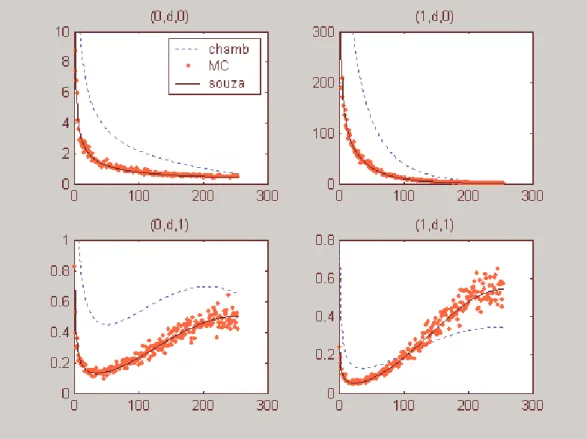
1 of Chambers (1998) as displayed in equations (3-4). Figure 2 shows the spectral function
derived in this note for aggregated stock ARFIMA processes and the one derived in Chambers
(1998), together with the periodogram ordinates averaged across 100 realizations of the process.
The X axis shows the indices j = 1, 2, …, T/2 representing the Fourier frequencies j2π/T. Figure 3 does the same as Figure 2, but for flow processes. The processes are aggregated from
ARFIMA(0,0.3,0), with n = 3; ARFIMA(1,0.3,0) with φ = 0.8 and n = 4; ARFIMA(0,0.3,1) with θ = -0.8 and n = 4; ARFIMA(1,0.3,1) with φ = -0.4, θ = -0.8 and n = 3. The aggregated series length is 512 observations and the error variance is taken as σε2 = 1.
As we can see for both stock and flow aggregated ARFIMA processes the averaged
periodogram ordinates (dots) are scattered around the solid line, which represents the formulae
(7-8) derived in this note. The formulae derived in Chambers (1998) and displayed in (3-4),
represented by a dashed line, yields values somewhat different from the observed in the
simulation experiment.
3 – Discussion
This note aims at disputing some of the results derived in Chambers (1998), specifically
the spectrum of temporal aggregates of discrete-time long memory processes. The main point is
that the aliasing effect was not taken into account. I provide here the corresponding spectrum in
light of the aliasing effect. A small simulation provides evidence in my favor.
As a result, two of the implications of Chambers (1998) results must be reviewed. First,
aggregation of flow variables, as the moving average filter (1 + B + … + Bn-1) assigns weights equal to zero to the frequencies which will alias right onto the frequency zero and very small for
those aliasing on its vicinity. For aggregation of stock variables, if d is positive, the unbounded energy in the spectrum for low frequencies in the original process dominates the energy coming
from aliases of these low frequencies in the aggregated process (if this energy is bounded), and a
condition similar to (1) still holds with same parameter d. However, if aggregating a stock variable with negative d, the condition (1), that implies a zero in the frequency zero, will surely be destroyed, unless in the very unlikely case where the spectrum in the frequencies which will
alias on the frequency zero is zero. A curious note is that, if long memory is defined in the time
domain as a hyperbolical decay of the autocorrelations,
(9) ρk ~ck2d−1ask→∞,
temporal aggregation of either type (stock or flow) is not able to destroy this property, and not
even to change the integration order d. This result, however, is of lesser practical importance because a negative d is rarely observed empirically, but arises frequently from overdifferencing a process. As practitioners usually aggregate series before differencing them and not otherwise, it
is unlikely that a (stock) process with negative d will be aggregated.
The second implication to be reviewed is the second testable hypothesis of Chambers
(1998, Section 2.5). He argues that the order of integration should be the same when estimated
from different frequencies of the data. This is true for flow variables but not for stock ones. Even
though the aggregation of stock variables retains the spectrum behavior in a small neighborhood
of zero if d > 0, the aggregation of flow variables do it in a far wider neighborhood, irrespective of the sign of d. These different frequency-domain behaviors of stock and flow variables will distinctly affect the (semiparametric) estimation of aggregated fractionally differenced processes
based on the low-frequency periodogram ordinates. If the process is a flow variable, less bias is
likely to be induced by aggregation, while if it is a stock variable, it is likely that aggregation
will incur some bias. In particular, if d < 0, the aggregation of stock fractionally integrated processes will destroy condition (1). However, for positive d, when the sample size increases the bias tends to disappear as a narrower band of frequencies is used for estimation. These
Appendix – Proof of Theorem 1
The spectrum of a covariance stationary discrete-time process Xt is defined by:
∞ −∞ = − = k ik x k x e
f γ ω
π ω
2 1 )
( , -π < ω ≤ π (A1)
where γkx is the k-th order autocovariance of Xt. As the autocovariance function of real valued
processes is an even function, (A1) reduces to:
∞ −∞ = = k x k x k
f γ ω
π
ω cos
2 1 )
( , -π < ω ≤ π. (A2)
The spectrum fx(ω) is then defined as a Fourier cosine series whose coefficients are the
autocovariances of Xt. As cos kω, k = 0, 1, 2, ..., is a complete orthogonal set over the interval (– π, π] for even functions (and the spectral density is an even function) the relation given by (A2) is equivalent to:
,... 2 , 1 , 0 ), ( cos cos ) ( = = ± ± = − − k dF k d k
fx x
x k π π π π ω ω ω γ (A3)
where Fx(ω) is the spectral distribution function of Xt. Consider first the aggregation of stock
variables. The autocovariances of Yt = Xntare given thus by:
,... 2 , 1 , 0 ), ( cos cos ) ( = = ± ± = = − − k dF nk d nk
fx x
x nk y k π π π π ω ω ω γ γ (A4)
First take the simpler case where n is an odd number. The integral in (A4) can be split into: − − − = − − − − = + − + + = = 2 1 2 1 / / 2 1 2 1 / ) 1 2 ( / ) 1 2 ( ) / 2 ( ) 2 cos( ) ( cos n n j n n x n n j n j n j x y
k j n
✁ dF jk nk ✁ dF nk π π π π π π ω ω
γ (A5)
Since cos(a + 2jπ) = cos(a), where j is an integer number, (A5) rewrites to: − − − = − + = 2 1 2 1 / / ) / 2 ( ) cos( n n j n n x y
k j n
✁ dF nk π π π ω γ (A6)
Making λ= nωwhere λ is the frequency measured in the time unit of Yt, we have:
− − − = − + = 2 1 2 1 ) / 2 / ( 1 ) cos( n n j x y
k dF n j n
n k π π π λ λ
γ (A7)
However, by (A3) we can write the k-th order autovariance of Yt as:
,... 2 , 1 , 0 ), ( cos cos ) ( = = ± ± = − − k dF k d k
fy y
The fact that cos kλ, k = 0, 1, 2, ..., is a complete orthogonal set over the interval (–π, π] for even functions, together with (A7) and (A8) imply (5) with g(n,ω) = 1.
Now if n is an even number (A5) rewrites to:
− − = − = − + + + + + + = 1 2 2 / 0 2 2 1 0 / ) / 2 ( ) 2 cos( ) / 2 ( ) 2 cos( n n j n x n n j n x y k n j dF jk nk n j dF jk nk π π π π ω π π ω γ (A9)
and the rest of the proof (for stock processes) follows as in the case n is odd.
Now consider the aggregation of flow variables. Let − = = 1 0 n j t j
t B X
Z be the overlapping
aggregated process of Xt. The moving average representation of (1 + B + … + Bn-1)
straightforwardly gives the following relationship between the spectra of Zt and Xt:
2 1 0 ) ( ) ( − = − = n k ik x
z f e
f ω ω ω , -π < ω ≤ π.The multiplicative term
2 1 0 − = − n k ik
e ω is equivalent to
) ( . 2 ) 2 / ( ) 2 / ( lim 2 2 ω π θ θ ω
θ nFn
sin n sin
=
→ . This latter result can be easily verified (see, for example,
Bloomfield 1976, p. 51). Now, the aggregated process Yt is obtained from Zt through an
aggregation of the stock type, and the relationship between the spectra of Yt and Xt is that given
References
Bloomfield, P., 1976, Fourier Analysis of Time Series: An Introduction (Wiley, New York).
Chambers, M. J., 1998, Long memory and aggregation in macroeconomic time series,
International Economic Review 39, 1053-1072.
Granger, C. W. G. and R. Joyeux, 1980, An introduction to long memory time series models and
fractional differencing, Journal of Time Series Analysis 1, 15-29.
Hamilton, J. D., 1994, Time Series Analysis (Princeton University Press, New Jersey).
Hosking, J., 1981, Fractional differencing, Biometrika 68, 1, 165-176.
Koopmans, L.H., 1974, The Spectral Analysis of Time Series (Academic Press, New York).
Oppenheim, A. V. and R. W. Schafer, 1989, Discrete-Time Signal Processing, (Prentice-Hall,
New Jersey).
Priestley, M. B., 1981, Spectral Analysis and Time Series (Academic Press, London).
Souza, L. R. and J. Smith, 2002, Bias in the memory parameter for different sampling rates,
International Journal of Forecasting 18, 299-313.
Souza, L. R. and J. Smith, 2003, Effects of temporal aggregation on estimates and forecasts of
fractionally integrated processes: A Monte Carlo study, International Journal of
Figure 1: The Fejer kernel for n = 6, restricted to (-π, π]