DEVELOPMENT OF A CONCEPTUAL DESIGN METHODOLOGY
FOCUSED ON SOLAR AIRCRAFTS
Dissertação apresentada ao Programa de Pós-Graduação em Engenharia Mecânica da Universidade Federal de Minas Gerais, como requisito parcial à obtenção do título de Mestre em Engenharia Mecânica.
Área de concentração: Projeto Mecânico.
Orientador: Prof. Dr. Paulo Henriques Iscold Andrade de Oliveira. DEMEC UFMG
Belo Horizonte
DEDICATÓRIA
Muito aprendi na UFMG sobre engenharia aeronáutica, o que tem sido muito importante. Este trabalho é dedicado a quatro senhores que foram fundamentais para o meu aprendizado, além da UFMG, sobre o que é um avião. Estas são
José Barbosa Filho, meu pai, Joseph Kovács,
José Renato Melo, e Yoshihiro Hamada.
Este trabalho é dedicado a estas pessoas que, além de terem me tornado um melhor engenheiro, fundamentalmente me tornaram um melhor ser humano.
AGRADECIMENTOS
Oh, I have slipped the surly bonds of earth
And danced the skies on laughter
–
silvered wings;
Su
ard I’ e li
ed, a d joi ed the tu
li g
mirth
Of sun-split clouds-and done a hundred things
You have not dreamed of-wheeled and soared and swung
High in sunlit silence. Hovering there,
I’ e hased the shouti g i d alo e, a d flu g
My eager craft though footless halls of air.
Up, up the long, delirious, burning blue
I’ e topped the i ds ept heights ith easy gra e
Where never lark, or even eagle flew.
A d, hile ith sile t, lifti g i d I’ e trod
The high untrespassed sanctity of space,
Put out my hand, and touched the face of God.
INDEX
DEDICATÓRIA ... 3
AGRADECIMENTOS... 4
LIST OF FIGURES ... 8
LIST OF TABLES ... 13
LIST OF SYMBOLS ... 14
RESUMO ... 19
ABSTRACT ... 20
1) INTRODUCTION ... 21
2) MOTIVATION ... 22
2.1) Reasons to perform solar research in Brazil ...22
2.2) Reasons to study solar aircraft ...24
2.3) Reasons to consider solar aircraft in a historical perspective ...26
3) LITERATURE REVIEW ... 31
3.1) Literature Review of Low Speed, Pioneer Aircraft ...31
3.2) Literature Review of Solar Aircraft ...32
3.3) Literature Review of Propellers ...37
3.4) Literature Review of Lift, Drag, Performance ...38
3.5) Literature Review of Reynolds Number effects ...39
3.6) Literature Review of Solar Incidence Model...51
3.7) Literature Review of Atmosphere ...52
3.8) Literature Review of Solar Aircraft Systems ...56
4) METHODOLOGIES ... 61
4.1) Overview ...61
4.2) Reference Systems ...62
4.3) Characterization of Solar Aircraft ...62
4.4) General Rules for Maximum Wing Load of Solar Aircraft ...66
4.5) Method for Solar Aircraft Design...73
4.6) Comment on Influence of Reynolds Number on Lift and Drag ...77
4.7) Simplified Methodology for Airfoil Preliminary Analysis ...80
4.8) Methodology for Propeller Studies ...87
4.9) Methodology for Drag Analysis ...94
4.11) Solar Aircraft Typical Mission Analyses ...106
4.12) Solar Incidence Model ...113
4.13) Mass Estimation: Method and assumptions ...122
5) STUDIES ... 132
5.1) Checking the limits of a Sun-powered aircraft. ...132
.2) Drag, Propulsio , Perfor a ce of Already-Flow Low-Speed Aircraft ...139
6) RESULTS ... 159
6.1) Requirements for the Conceptual Design of the three Solar Aircraft ...159
6.2) Example of the Design Parameters Definition Iterative Process ...160
6.3) Definitions for the New designs ...163
6.4) Example of Mission Analysis...167
6.5) Diagrams of Flyable Region and Long Endurance Region ...181
7) CONCLUSIONS ... 185
7.1) Overall ...185
7.2) Next Steps ...186
8) REFERENCES ... 187
8.1) References Related to Early Aviation Pioneer Aircraft ...187
8.2) References Related to Solar and Man-Powered Aircraft ...188
8.3) References Related to Drag, Lift, Performance, Atmosphere and Mass Analysis ...192
8.4) References Related to Propeller Analysis ...195
LIST OF FIGURES
FIGURE Description Page
Figure 2.1: Mean Daily Solar Energy Intensity MDSI in some of Earth‟s countries. 22 Figure 2.2: Mean Daily Solar Energy, MDSIxArea in some of Earth‟s countries. 23 Figure 2.3: Advancement of solar aircraft in terms of altitude over time. 25 Figure 2.4: Advancement of solar aircraft in terms of endurance over time. 25 Figure 2.5: Advancement of solar aircraft in terms of range over time 26 Figure 2.6: Values of aircraft maximum mass along time; solar aircraft are included
for comparison.
28
Figure 2.7: Aircraft wing loading growth along time. Solar aircraft are included for comparison.
29
Figure 2.8: Power loading of the aircraft presented in the previous pictures along time. 29 Figure 2.9: Aspect Ratio of the aircraft presented in the previous pictures along time. 30 Figure 3.1: Sunrise drag polars reduced from flight trials 36
Figure 3.2: Sunrise I expected altitude profile 37
Figure 3.3: Variation of CL with Re for Cambered Plate and a Conventional Airfoil 41 Figure 3.4: Variation of CD with Re for Cambered Plate and a Conventional Airfoil 41 Figure 3.5: Variation of L/D with Re for Cambered Plate and a Conventional Airfoil;
values are consistent with the ones presented in figures 3.5-1a and 3.5-1b
42
Figure 3.6: Cambered plate „417a‟ and airfoil N-60, from Schmitz (1942) 42 Figure 3.7: Airfoils from two aircraft designed by Paul MacCready; „Lissaman 7769‟
(above) for Gossamer Condor, and „Lissaman-Hibbs 8025‟ for Solar Challenger.
43
FIGURE Description Page Figure 3.20: Variation with altitude, of sunlight irradiance reduction due to atmosphere;
Sun positioned at the zenith, and the sky without clouds.
54
Figure 3.21: Variation with altitude of the Sun irradiance; Sun positioned at the zenith, and the sky without clouds.
55
Figure 3.22: Sketch of the general propulsive chain in a sun-powered aircraft. 56 Figure 3.23: Specific mass of different types of batteries for Solar aircraft; lead-acid are
presented only for comparison
58
Figure 3.24: Mass/Area ratio of solar cells from different solar aircraft. 58 Figure 3.25: Power/Area and Power/Mass ratios of solar cells from different solar
aircraft.
59
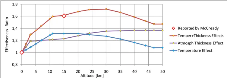
Figure 3.26: Mass/Power ratio of engines from different solar aircraft. 59 Figure 3.27: Changes in solar cells effectiveness in function of the altitude,
due to atmosphere thickness and temperature effect
60
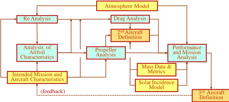
Figure 4.1: Simplified view of the link between the methodologies in the design and analysis process
61
Figure 4.2: Comparison of payload-endurance diagrams from conventional and sun-powered aircraft
63
Figure 4.3: Comparison of specific payload - endurance diagrams from conventional and solar aircraft
64
Figure 4.4: Comparison of payload-altitude diagrams from conventional and sun-powered aircraft
64
Figure 4.5 Comparison of specific payload - altitude diagrams from conventional and solar aircraft
65
Figure 4.6: Procedure for of the definition and check of batteries capability 73 Figure 4.7: General Flowchart Considered for Solar Aircraft Definition and Design. 74 Figure 4.8: Survey of Re of Wing and Propellers, of several aircraft analyzed
in this work
78
Figure 4.9: Kabr in function of camber ratio Z/C 81
Figure 4.10: CDo 2D in function of thickness ratio T/C and Reynolds Number. 81 Figure 4.11: CDoshape in function of thickness ratio T/C and camber ratio Z /C. 82 Figure 4.12: CDoRe in function of Reynolds number, for fully turbulent flow
and intermediate flow.
82
Figure 4.13: in function of camber ratio Z/C 84
Figure 4.14: in function of thickness ratio T/C and Reynolds Number 84
Figure 4.15: in function of thickness ratio T/C 85
Figure 4.16: Multiplying factor f for CLmax. 86
FIGURE Description Page
Figure 4.19: Flowchart for propeller evaluation 88
Figure 4.20: Propeller Blade, with a blade element „AB‟ (left);
and the local wind speeds at that blade element „AB‟ (right)
89
Figure 4.21: Same propeller blade element „AB‟ from figure 4.4-2; but now presenting the local angles and α, and the local Lift
and drag forces (left);and the components of the local resultant aerodynamic force into tangential and axial forces (right) .
90
Figure 4.22: Stream tube of air flow passing by propeller disk; aircraft flying from right side to left
91
Figure 4.23:. Example of CL distribution as output from the lifting line model, for a rectangular wing of aspect ratio of 24.
96
Figure 4.24: Definition of additional induced drag coefficient δ for non-elliptical wings 97 Figure 4.25: Non-dimensional incremental speed due to propeller thrust along
longitudinal axis.
99
Figure 4.26: Variation of speeds along longitudinal axis for several aircraft speed ratios TAS/∆V.
101
Figure 4.27: Example of Stream Tube of Propeller Stream definition; 14-Bis aircraft. 102 Figure 4.28: Example of Stream Tube of Propeller Stream definition; 14-Bis aircraft. 102 Figure 4.29: General relationship between the main characteristics and data,
related to Solar Aircraft Analysis
107
Figure 4.30: Mission Simulation Flowchart, one time interval: Aircraft Type 1, without batteries.
108
Figure 4.31: Mission Simulation Flowchart, one time interval: Aircraft Type 2, with batteries.
109
Figure 4.32: General Flowchart Considered for the Solar Incidence Evaluation. 114 Figure 4.33: Basic elements for Earth attitude related to Sun 115 Figure 4.34: Solar Cone for June, and local surface corresponding to Latitude 19.92 S. 116 Figure 4.35: Solar Cone for Sept. or March, and local surface corresponding to
Latitude of 19.92 S.
117
Figure 4.36: Solar Cone for December, and local surface corresponding to Latitude of 19.92 S.
117
Figure 4.37: Hour of sunrise for several latitudes on the southern hemisphere in function of the year weeks
118
Figure 4.38: Sun daily energy incident in a horizontal surface on the ground, at sea level, for several latitudes of southern hemisphere, from December to June.
119
Figure 4.39: Distribution of solar power in function of hour of the day and Latitude, in December, at the southern hemisphere
120
Figure 4.40: Solar power density in function of hour of the day and Latitude, in June, at the southern hemisphere
FIGURE Description Page Figure 4.41: Results of solar irradiance above atmosphere, Earth, latitude 20 north. 121 Figure 4.42: Calculated solar power curve for a specific day and latitude,
compared with the one obtained from Roland Boucher (2003)
121
Figure 4.43: Take-off mass comparison of solar aircraft representatives 129 Figure 4.44: Mass breakdown comparison of solar aircraft representatives 129 Figure 4.45: Diagram of Wing Structural Mass versus MTOW x A1/2 131 Figure 5.1: A hypothetical Solar Aircraft (left) with the same wing area and aspect ratio
of the Airbus A-380 aircraft (right)
133
Figure 5.2: Values of M/S max obtained for different SAR values, aircraft with batteries. 135 Figure 5.3: Maximum horizontal flight altitudes; comp. betw. calculated and intended values 137 Figure 5.4: Calculated maximum altitudes for continuous flight at constant altitudes 138 Figure 5.5: Calculated Maximum wing loadings for continuous flights,
at a constant altitude of 3Km, compared with the real wing loadings.
138
Figure 5.6: Santos-Dumont N.9 „Balladeuse‟ Airship 141
Figure 5.7: Evaluation of CDo of vehicle items, in function the thickness ratio t/c and the Reynolds number
142
Figure 5.8: Pie-Chart Diagram of the SD N.9 Balladeuse Parasite Drag Breakdown 142
Figure 5.9: Propeller blade airfoil geometry 143
Figure 5.10: Propeller blade planform, and 3 possible pitch angle variations 143 Figure 5.11: Reynolds number evaluation for three propeller sections. 144 Figure 5.12: Three-dimensional coefficients CL and CD of the propeller airfoil,
in function of α local.
144
Figure 5.13: Curves of CT versus J for the three pitch angle distributions. 145 Figure 5.14: Curves of CP versus J for the three pitch angle distributions. 145 Figure 5.15: Curves of ηprop versus J for the three pitch angle distributions. 146 Figure 5.16: Curves of drag and maximum thrust in function of airspeed, and
VH determination.
146
Figure 5.17: Comparison of drag polars of six low-wing load aircraft 148 Figure 5.18: Drag and Thrust versus Speed for the analyzed aircraft 149 Figure 5.19: Comparison between calculated and reported values of
performance parameters for the some of the aircraft studied
149
Figure 5.20: Sunrise I without solar array, comparison between drag polar curves: theoretical and from tests
150
Figure 5.21: Sunrise II with solar array, drag polar curves; comparison between the curve reduced from flight trials, and the theoretical ones obtained through this work.
152
Figure 5.22: Comparison between calculated values (continuous lines) and
the ones reduced from flight Tests for Sunrise I sink rate and glide rate.
153
Figure 5.23: Sunrise I climb rate curves. Comparison between the one from Flight Tests and two ones calculated.
FIGURE Description Page Figure 5.24: Sunrise I, comparison of mission altitude profile for 21June, California, USA;
calculated values and expected from the designers
155
Figure 5.24: Sunrise I, mission analysis: Rate of climb and solar intensity,21 june , California, USA
155
Figure 5.25: Sunrise I, mission analysis: Rate of climb (output) and solar intensity at jun21, California (input).
156
Figure 5.27: Sunrise I, mission altitude profile, sensitiveness studies; 21June, Calif., USA 157 Figure 5.28: Sunrise I, mission altitude profile, sensitiveness studies; 21June,
California, USA, all runs
158
Figure 6.1: Visualization of the parameter values variation throughout the iterative design process of the Method of Solar Aircraft for the Travel Flight aircraft; Total Mass represented at left axis, wing area at right axis.
161
Figure 6.2: Sport Flight Solar Aircraft Proposal 164
Figure 6.3: Travel Flight Solar Aircraft Proposal 165
Figure 6.4: High Flight Solar Aircraft Proposal 166
Figure 6.5: High Flight mission time history: Altitude [kft] vs time [hs] 171 Figure 6.6: High Flight mission time history: TAS [km/h] vs time [hs] 171 Figure 6.7: High Flight mission time history: acceleration in path direction [m/s2]
vs time [hs]
172
Figure 6.8: High Flight mission time history: Lift-to Drag ratio vs time [hs] 172 Figure 6.9: High Flight mission time history: Propeller thrust [N] vs time [hs] 173 Figure 6.10: High Flight mission time history: Propeller RPM vs time [hs] 173 Figure 6.11: High Flight mission time history: Propeller effectiveness vs time [hs] 174 Figure 6.12: High Flight mission time history: Available power and horizontal flight
power, vs time [hs]
174
Figure 6.13: High Flight mission time history: Same figure as 6.4-8, but adding the necessary power to accelerate vs time [hs]
175
Figure 6.14: High Flight mission time history: Cells output power,
power delivered to air, power from batteries to air, vs time [hs]
175
Figure 6.15: High Flight mission time history: Rate-of-climb [fpm] vs time [hs] 176 Figure 6.16: High Flight mission time history: [degrees] vs time [hs] 176 Figure 6.17: High Flight mission time history: Re at wing and propeller vs time [hs] 177 Figure 6.18: High Flight mission: Altitude [kft] vs TAS [km/h] 178 Figure 6.19: High Flight mission: Propeller effectiveness vs advance ratio „J‟ 179 Figure 6.20: High Flight mission analysis: Propeller RPM vs power delivered to air [Watt] 179 Figure 6.21: High Flight mission analysis: Propeller RPM vs engine output power [Watt] 180 Figure 6.22: High Flight mission analysis: Propeller RPM vs air temperature [Celsius] 180 Figure 6.23: Maximum altitude in function of latitude and month for the High Flight
aircraft; southern hemisphere.
182
Figure 6.24: Minimum altitude in function of latitude and month for the High Flight aircraft; southern hemisphere.
183
Figure 6.25: Daily distance flown in function of latitude and month for the High Flight aircraft; southern hemisphere.
LIST OF TABLES
TABLE Description Page
Table 3.1: List of some of the references about solar and HPA aircraft consulted 33
Table 3.2: Simplified and conceptual values of the propulsive chain for three different aircraft
57
Table 4.1: Solar Aircraft Mass Distribution Evaluation: Input Data 126
Table 4.2: Solar Aircraft Mass Distribution Evaluation: Calculated Values 126
Table 4.3: Pioneer Aircraft Parameters 127
Table 4.4: Sailplane Mass Distribution Evaluation: Input Data 127
Table 4.5: Sailplane Mass Distribution Evaluation: Calculated Values 127
Table 5.1: Summary of the types of Analyses performed for the Low Speed Aircraft 140
Table 5.2: Parametric studies for Sunrise I Mission Analysis 157
Table 6.1: Data and Constraints Pre-Defined for the Conceptual Design of Three Different Types of Solar Aircraft
161
Table 6.2: Parameters Obtained from Conceptual Design of Three Types of Solar Aircraft 162
Table 6.3: Example of main data for mission analysis 168
LIST OF SYMBOLS
International System of units has been used unless otherwise indicated.
Symbol or
Abbreviation Value and Unit Description
MPPT Maximum power point tracker
VS Stall speed
VNE Never exceed speed
Kft Thousand feet
Ppm Parts per million
R* 8.31446 J/(K.mol) Ideal gas constant
MM kg/kmol Molecular Mass
K Kelvin degrees
Km kilometer
H Hour
s Second
W Watt
ρ, rho Kg/m3 Atmosphere local specific mass T oC, oK Temperature
Tr N Thrust
TAS, V m/s, km/h True Airspeed EAS m/s, km/h Equivalent Airspeed
P N/m2 Pressure
Pw W, hp Power
ν Atmosphere local kinematic viscosity
µ Friction coefficient, atmosphere local dynamic viscosity
NAA National Aeronautical Association
Symbol or
Abbreviation Value and Unit Description
NASA National Aeronautics and Space Agency
NASA CR NASA Contractor Report
NASA TM NASA Technical Memorandum
NASA TN NASA Technical Note
AIAA American Institute of Aeronautics and Astronautics NOAA National Oceanic and Atmospheric Administration
USAF United States Air Force
HPA, MPA Human-powered aircraft , Man-powered aircraft
L Newton Lift force
D Newton Drag force
CL Lift coefficient
CD Drag coefficient
CDo Drag coefficient for zero lift
CDmin Minimum drag coefficient
CLmax Maximum lift coefficient
CLo Lift coefficient for α=0
2D Index for two-dimensional
Re, R.N. Reynolds Number
A Aspect Ratio
e Oswald efficiency factor
CLα 1/rad, rad-1 Derivative of lift coefficient related to angle of attack α, alpha degree or radian Angle of attack
T/C, t/c Airfoil thickness ratio Z/C, z/c Airfoil camber ratio ratio
z meter Max. vertical distance of airfoil camber line from chord line t meter Maximum vertical thickness of airfoil
C, c meter Airfoil chord length
CMG Mean Geometric Chord
Symbol or
Abbreviation Value and Unit Description Alt, H km, m, feet Altitude
X, Y, Z meters Aircraft coordinates
E L/D, lift-to-drag ratio
E* Maximum lift-to-drag ratio
CL* CL for maximum lift-to-drag ratio
CL** CL for minimum horizontal flight power E** E for minimum horizontal flight power APw W power available to be delivered to the air
RPw W Required Power to perform horizontal flight; D x TAS
DAE W.h Daily Available Energy
DRE W.h Daily Req Energy
MOLA Mars Orbiter Laser Altimeter
Re Reynolds Number
MDSI kW.h/m2 Mean Daily Solar Intensity
SAR Solar array to wing area ratio
ILSPI W./m Instantaneous and local Sun power intensity SLDEI W.h/m Solar Local Daily Energy intensity
CLsaf Limitation of high CL for safety in terms of stall avoidance
G Gravity acceleration
ηeng Engine efficiency
ηprop Propeller efficiency
ηsist System efficiency, aircraft with batteries
ηsisb System efficiency, aircraft with batteries
SHP hp Propeller shaft power
δ Additional induced drag factor for non-elliptical wing degrees Local wind angle over propeller blade section
Faxi Newton Axial force at each strip
Symbol or
Abbreviation Value and Unit Description
, beta, degrees Propeller blade local pitch angle
beta75 degrees Propeller blade pitch angle at 75% of radius
Nb Number of blades
Ns Number of strips
Ri meters Distance from propeller strip to rotation axis
∆V m/s Final Incremental speed due to propeller thrust
CT, Ct Propeller Thrust Coefficient
CP, Cp Propeller Power Coefficient
J Propeller Advance Ratio
Sref m2 Reference area for Drag coefficients k meters Induced drag coefficient factor Sdisk m2 Propeller Disk Area
D m Propeller Diameter
Vdisk m/s Air speed at Propeller Disk
Sstm m2 Local Area of the propeller stream tube
Vstm m/s Local incremental speed at the propeller stream tube Dstm meters Local Diameter of the propeller stream tube
fv Multiplying factor for take-off speed related to minimum speed ax m/s2 Acceleration in X direction
Dg Newton Drag due to wheels and skid contact with ground N Newton Ground normal upward force
degrees Aircraft attitude angle during Take-off run Newton Maximum Thrust for the specific speed
Symbol or
Abbreviation Value and Unit Description
P1 Seconds Initial time of the time interval; in the Mission Analysis P2 Seconds The final time of the time interval, in the Mission Analysis PM Seconds The average time of the time interval, in the Mission Analysis
a-p angle degrees Angle between planet‟s revolution axis, and the normal to the plane of planet‟s orbital translation around the Sun.
SEL Sun-Earth Line
MEng kg Engine Mass
PwEng W Engine Power
MBat kg Mass of Batteries MCell kg Mass of Solar Panels
SCell m2 Area of Solar Panels
MStr , Mstr kg Mass of aircraft Structure, airframe mass
MContrl kg Mass of the Control Systems, including electrical transmission controls
WSM kg Wing Structural Mass
N, S North and South Latitudes
Msys kg Mass of Aircraft Systems
Mpayl kg Payload Mass
UIUC University of Illinois at Urbana-Champaign GRASS Geographic Resources Analysis Support System
RESUMO
ABSTRACT
1) INTRODUCTION
A solar aircraft, or Sun-powered aircraft can be defined as an atmospheric vehicle that can move horizontally due to the power extracted from sunlight through photovoltaic cells dispersed in its external surfaces. A power chain inside the vehicle transforms the light energy received from the sun in electrical energy, which is transformed into the mechanical energy by a electrical motor, and is delivered to the surrounding gaseous mean through a rotating propeller. The resulting forward thrust balances the drag related to two main sources, the forward movement, and the aerodynamic lift that balances the vehicle weight. Successful solar aircraft - manned or unmanned - are something new in aviation. The first successful attempts have occurred by 1970 and 1980 decades.
The low power which can be extracted from the sun by aircraft surfaces is very low when compared to the power of conventional internal combustion aircraft. As a result of this fact, a solar aircraft must be, in terms of mass, wing loading, speeds, structures, and other design criteria, remarkably different from the conventional, internal combustion aircraft. The ways to think, design and operate a solar aircraft shall be different – at least in some aspects – than a internal combustion aircraft.
Related to this aspect, several questions can be made. For example: In which aspects solar aircraft can be though by the same viewpoint than a conventional aircraft? Which aspects, from the ones that solar aircraft differ from conventional aircraft, are the most relevant for design and operation studies? Which are the missions that solar aircraft could be useful or advantageous in the present and near future scenario? Can the solar aircraft be used in only one type of operation, or there are different potential fields of use? Is it possible to obtain a methodology for the initial definition of solar aircraft? In which point the nowadays technologies are mature to design a solar aircraft? What should be the critical technologies to take into account in specific the design of a solar aircraft?
2) MOTIVATION
This chapter presents three main aspects that stimulated this work, and shaped the way it has been developed.
2.1) Reasons to perform solar research in Brazil
A simplified study has been performed by the author in order to obtain an overall picture of solar power distribution on the Earth‟s Countries. The main results of this study are presented in the following figures.
The solar most relevant information in author‟s viewpoint is presented in figure 2.1 in which the Mean Daily Solar Intensity MDSI is compared for several countries. This parameter represents the energy received during a day per square meter, and can be expressed in kW.h/m2 .
Figure 2.1: Mean Daily Solar Energy Intensity „MDSI‟ in some of Earth‟s countries. 3,0 3,5 4,0 4,5 5,0 5,5 6,0 6,5 7,0 B ra zi l C ol om bi a Ve ne zu el a Pe ru Su da n In di a M ex ic o A us tr al ia A lg er ia C hi na U SA Ja pa n A rg en ti na Su it ze rl an d G er m an y C an ad a UK R us si a
One can see by the figure 2.1 that Brazil presents a high level of daily solar energy intensity when compared to other countries. By this figure it can be observed that Brazil receives per square meter roughly 31% more energy from the Sun than USA, 56% more than Switzerland, 70% more than Germany , 79% more than Canada, United Kingdom (UK) and Russia.
This scenario turns to be even more dramatic if the total energy that sun provides to a country is calculated, i.e. taking into account the country‟s area. Although this parameter can be questionable for some, even only as a reference, it is interesting to be accounted for. The Mean Daily Solar Energy, which corresponds to the product MDSI x Area is presented, in terms of GW.h, in figure 2.2, for the same countries selected for presentation in figure 2.2. By observing figure 2.2, one can obtain that Brazil presents about 29 times the value of Japan, 39 times the value of Germany, 60 times the value of UK and more than 300 times the value of Switzerland.
Figure 2.2: Mean Daily Solar Energy, MDSI x Area in some of Earth‟s countries.
Avoiding discussion of which metrics are the most applicable, the one from figure 2.1 or figure 2.2, it can be said that it is possible to use any of the two to achieve the same conclusion:
Countries, as remarkably Germany and Switzerland, that have obtained several important results in terms of Solar power research, are less favored by Sun than Brazil; and
100 1000 10000 100000 R us si a B ra zi l C hi na U SA A us tr al ia C an ad a In di a Su da n A lg er ia A rg en ti na M ex ic o Pe ru C o lo m b ia Ve ne zu el a Ja pa n G er m an y UK Su it ze rl an d
Brazil, which such large solar potential, should also increase efforts in this direction of solar power research.
2.2) Reasons to study solar aircraft
The figures 2.3 to 2.5 present the evolution of the values of altitude, flight time and flight distance achieved by solar aircraft, from the first attempts (circa 1974) up to the present. In order to provide comparison, values for aircraft with combustion engines are also presented in the altitude and flight time figures. The figures show how fast the solar aircraft have progressed in terms of flight performance.
In figure 2.3 the advancement of Solar Aircraft in terms of altitude is presented and compared to typical altitudes of General Aviation and Commercial Aircraft, and the maximum altitude record for a combustion engine aircraft, the SR-71. In figure 2.3 only rocket-propelled or rocket-assisted aircraft are not considered. As can be seen in this figure, the highest altitude level achieved is from a solar aircraft.
In figure 2.4 the advancement of Solar Aircraft in terms of non-refueling flight time is presented, and compared to typical endurance levels of General Aviation and Commercial Aircraft; and the level of the maximum endurance for a combustion engine aircraft, the Rutan Voyager, is also presented. In this figure, only the aircraft which are heavier than air and intended for atmospheric flight are represented. It is possible to observe in this figure the point of about 330 hours, occurred in 2010, significantly above the endurance level achieved by Rutan Voyager; so one can note that the maximum endurance flight for an atmospheric, heavier than air aircraft has been performed by a solar aircraft.
In order to avoid the interpretation of the figures 2.3 and 2.4 in an overoptimistic bias, and to provide a better understanding about the limitations of sun-powered aircraft, in the section 4.3 some performance figures related to aircraft payloads are additionally presents.
Figure 2.3: Advancement of solar aircraft in terms of altitude over time.
Figure 2.4: Advancement of solar aircraft in terms of endurance over time. 0
5 10 15 20 25 30 35
1970 1975 1980 1985 1990 1995 2000 2005 2010 2015
A
lt
it
ude
[
k
m
]
Year
Solar Aircraft General aviation Commercial aircraft Lockheed SR-71
0 50 100 150 200 250 300 350
1970 1975 1980 1985 1990 1995 2000 2005 2010 2015
Fl
ig
ht
T
im
e
[
hs
]
Year
Figure 2.5: Advancement of solar aircraft in terms of range over time
It can be seen from figures 2.3 and 2.4 that, either in terms of altitude and flight time, solar aircraft evolved in a fast way along few decades, and recently surpassed the maximum values hold by the aircraft with combustion engines. These two aspects - tendency of fast growing, and achievement of values beyond the ones of combustion propulsion aircraft - for the solar aircraft in terms of altitude and flight time, are high incentives for solar aircraft researches. Despite this, the - still modest - flight distances achieved by solar aircraft, whose evolution is presented in figure 2.5, can indicate a growth potential, and can be understood as one additional incentive and opportunity for solar aircraft research. So, there is also a great potential and opportunity for solar aircraft researches focusing range.
2.3) Reasons to consider solar aircraft in a historical perspective
The evolution of some parameters from the early days of well-succeeded manned glide flights, circa 1885, up to the present is shown in the figures 2.6 to 2.9. In the figures three types of aircraft, early gliders, combustion propulsion aircraft and solar aircraft, are represented.
The variation along time of values of aircraft maximum mass along and wing loading are presented in figures 2.6 and 2.7 respectively.
0 100 200 300 400 500 600 700 800 900 1000
1970 1975 1980 1985 1990 1995 2000 2005 2010 2015
D
is
ta
nc
e
[
k
m
]
Year
From the figure 2.6 it can be noticed that solar aircraft show some tendency of mass increasing, but definitively not as high as the one that occurred with the combustion-powered aircraft; additionally it can be noticed from the same figure that the present mass values are close to the ones developed up to 1915.
From the figure 2.7 it can be noticed a very interesting feature, mainly if one compares this aspect with the one observed for figure 2.6: In a different way from the aircraft mass (figure 2.6), the maximum values of solar aircraft wing loading (figure 2.7) apparently have not increased with time, after 1980. Additionally from figure 2.7 one can note that the steady wing loading values from Solar aircraft are significantly lower compared to nowadays combustion aircraft, and – as also occurs with mass values - the solar wing loading values are in the same magnitude than the wing loading values from early aviation (up to 1915) aircraft.
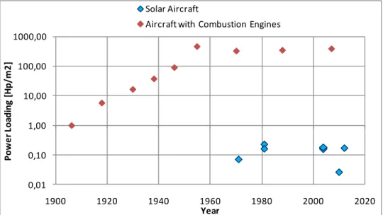
The figure 2.8 presents the variation of power loading with time of solar aircraft, compared to the power loading of combustion engine aircraft. From this figure one can note the same feature than the one observed from „wing loading‟ tendencies of figure 2.7: The power loading of solar aircraft seems to be steady, with a very low value if compared to nowadays combustion-powered aircraft. But one interesting new feature can observed in figure 2.8 which is different from the characteristics observed in figure 2.7 and 2.6: The steady power loading level for solar aircraft is one order of magnitude below the minimum values of combustion-powered aircraft. This can indicate how different this type of aircraft can be from the conventional, combustion-powered aircraft.
The Solar aircraft power loading levels presented in figure 2.8, significantly lower than conventional combustion-powered aircraft (even considering the earliest days of aviation) are one expression of the new and challenging aspects related to solar aircraft. And this can represent the needs of new ways of thinking, and new solutions in terms of arrangement, configuration, aerodynamics, structures and systems, compared to the existing combustion-powered aircraft.
The figure 2.9 presents the variation with time of solar aircraft wing aspect ratio, compared to the variation of the same parameter of combustion engine aircraft. From this figure one can note that solar aircraft present a tendency of increasing the wing aspect ratio to values notably higher than the typical ones from combustion-powered aircraft. These last ones presented the tendency of keeping this parameter steady along the last 70 decades. The high-aspect ratio tendency is one of the solutions associated to the very low power levels of solar aircraft compared to combustion-powered aircraft.
Solar aircraft are, among other features, in terms of power loading and aspect ratio, something new in aviation. But in terms of wing load and mass, they can be considered close to the aircraft of early days of aviation. Due to this aspect, it may be important to understand the solar aircraft not only in the new, technological aspects, but also in their similarities with early aviation representatives. In addition, tools intended for analysis of sun-powered aircraft can be also used for - and initially checked through - analysis of well known, early aviation representatives.
Figure 2.6: Values of aircraft maximum mass along time; solar aircraft are included for comparison. 1
10 100 1000 10000 100000 1000000
1880 1900 1920 1940 1960 1980 2000 2020
M
a
ss
[
k
g
]
Year
Solar Aircraft
Figure 2.7: Aircraft wing loading growth along time. Solar aircraft are included for comparison.
Figure 2.8: Power loading of the aircraft presented in the previous pictures along time. 1
10 100 1000
1880 1900 1920 1940 1960 1980 2000 2020
W
ing
L
oa
di
ng
[
k
g
/
m
2
]
Year
Solar Aircraft
Aircraft with Combustion Engines Early Gliders
0,01 0,10 1,00 10,00 100,00 1000,00
1900 1920 1940 1960 1980 2000 2020
P
ow
e
r
L
oa
di
ng
[
H
p/
m
2
]
Year
Solar Aircraft
Figure 2.9: Aspect Ratio of the aircraft presented in the previous pictures along time. 1
10
1880 1900 1920 1940 1960 1980 2000 2020
A
spe
ct
R
a
ti
o
Year
Solar Aircraft
3) LITERATURE REVIEW
In this chapter the most important sources to this work are identified and briefly commented. Since several areas of knowledge are involved in the researches performed, the contributions are presented as grouped by main areas, as follows.
3.1) Literature Review of Low Speed, Pioneer Aircraft
The pioneer aircraft considered in this work are some remarkable examples of well succeeded early aircraft from 1890 to 1910. Studies related to these aircraft have been included in this work - even considering that these aircraft are not Sun-powered - due to some similarities of these aircraft to solar aircraft, e.g. the very low speed and very low wing loading, as presented in the section 2.3. From the several publications studied, the ones which have been the most valuable ones are mentioned in this section. Some of the most valuable publications found in this area are from decades ago, as Lilienthal (1889), Baden-Powel (1903), Ferris (1910), Karlson (1940) and Villares (1957).
Lilienthal (1889) presents the airfoil shape and tests for evaluation of the aerodynamic forces at low Reynolds numbers, probably the first scientific research about cambered airfoils. Karlson (1940) also presents reliable information regarding Lilienthal aircraft. The site Otto Lilienthal Museum (2011) presents a vast and consistent data compilation of most of the Lilienthal aircraft, and articles written by Lilienthal for a nineteen-century magazine, explaining the concepts associated to the hang-gliding sport activities.
3.2) Literature Review of Solar Aircraft
As several valuable sources of this group have been considered in this work, in a number significantly higher than the sources related to the other areas, the most important ones are listed in the table 3.1, with the identification of the main point of relevance for this work. In this section the sources related to human powered flight are also included. The level of relevance of the information for the present work is also identified in table 3.1, in the priority order: high and important.
Specific comments about some of the sources are presented as follows.
The Site of Fédération Aéronautique Internationale (2014) presents the officially recognizable records, including the ones for Sun-powered aircraft.
Several highly valuable sources of information have been released by NASA. NASA sites (2010, 2014) present reliable and consistent information regarding the solar aircraft family from Pathfinder to Helios; NASA publications from Phillips (1980), Hall et al (1983, 1985), Hall and Hall (1984), Landis et al (2002), Colozza (1994), Bailey and Bower (1992), Penner (1983) address different aspects related to solar aircraft; in general focusing high-altitude flights. Besides NASA publications, additional information on Pathfinder systems can be found in Colella and Wenneker (1994).
In Noth (2007, 2008a) the most important aspects related to Solar aircraft design are described, together with a reliable design methodology. Based on this procedure, the aircraft sky-sailor has been designed, built and flown continuously 27 hs without the need of thermals (Noth, 2008a). Among several important and useful concepts presented in these sources, it is important to highlight some: The perceived absence of clear design methodologies related to some already-flown solar planes, the absence of prototypes to validate some of the published design methodologies, the drawbacks related to very small and very large solar aircraft, the limits of solar aircraft in terms of wing loading, the structural weight in function of wing area, the issues related to increase flight endurance by using altitude gain or thermal soaring.
story of Zephyr, the information presented by Cocconi (2008), Murray (2005), Dornheim (2005) about Solong aircraft; among other highly valuable ones.
Table 3.1: List of some of the references about solar and HPA aircraft consulted
Author Year of Publication
Type of Publication
Relevance
for this Work Main Points for Relevance
Noth, Sigwart,
Engel
1.1, 2007 Lecture
material High
concepts for solar aircraft design aimed to 24+ flights, used for Sky-Sailor
André Noth 2008 (a) Doctoral exam
presentation High General concepts for solar aircraft design
André Noth 2008 (b) Report High Sky-Sailor characteristics
André Noth 2008 (c) Report Important List with characteristics of 90+ solar powered aircraft
André Noth Jun2008 (d) Report Important Sky-Sailor Solar proved Continuous Flight
André Noth 2008 (e) www.
sky-sailor.ethz.ch High
Initial description of work; Important considerations of the solar flight on Mars; Access topublications related to Sky-Sailor.
Alan
Cocconi 2008 (a)
Informal
Report: High
Solong: Characteristics, and
strategies for the 48hs flight
Alan
Cocconi 2008 (b) Presentation High Concepts for solar aircraft engines
Hannes Ross 2009 (a) Presentation High Design concepts related to Solar Impulse
Hannes Ross 2009 (b) Paper High Design concepts related to Solar Impulse
Roland
Boucher 2003,
www.project
sunrise.info High
Data, history, mission and description of Sunrise I
NASA Accessed
2013 Fact Sheets (2) High Description of Helios family
Charles
Murray 2005
Design News
Magazine (1) High Description of Cocconi Solong
Michael Dornheim
26 Jun 2005
Aviation Week
Table 3.1 (continuation): List of some of the references about solar and HPA aircraft consulted
Author Year of
Publication
Type of Publication
Relevance for
this Work Main Points for Relevance
Piccard, Borschberg
2009 to present
www.solar
impulse.com High Data and facts of solar Impulse aircraft
Robert Boucher 1984
Paper : History of Solar Flight
High Data of SunriseII, Solar Riser, Solar One, Gossamer Penguin, Solair I, S.Challenger
Robert Boucher 1985 Paper High History and Data of Sunrise I and Sunrise II
McCready, Lissaman,
Morgan
1983 Paper High Solar Challenger: Design and test results
Annabel Rapinett 2009 M Sc
dissertation High Zephyr: History, systems, launching
Colella,
Wenneker 1994
Magazine
R&TR Important Technical solutions for Pathfinder
NASA 1998 NASA Facts
PDF Important
Solar Research at Dryden Center, Helios Family
Manish Bhatt 2012 M Sc research Important Design of a long endurance, high altitude solar aircraft
Benedet 1985 NASA TM, M
Sc Thesis Important
Description of solar cells, main principles of solar aircraft and examples of solar aircraft,
report made in Argentina
Montgomery
Mourtos 2013 Paper Important Design example: Photon aircraft
Héctor Vidales 2013 M Sc thesis Important Basic concepts and examples aircraft systems definition
Yaser Najafi 2011 M Sc research Important Design of a long endurance solar aircraft
Jabbas,
Leutenegger 2010 paper Important
Design techniques, flyable envelope; Solar aircraft data
Eric Raymond Accessed 2013
www.
solar-flight.com Important
Description and missions of Sunseeker aircraft; description of Edelweiss sailplane
Martin Cowley 1981 Aeromodeler
Magazine Important
Table 3.1 (concluded): List of some of the references about solar and HPA aircraft consulted
Author Year of Publication
Type of Publication
Relevance for
this Work Main Points for Relevance
Moulton,
Lloyd,Cowley Sept. 1979
Aeromodeler
Magazine Important Description of the Gossamer Albatross
Shiau, Ma,
Chiu, Shie 2010 Paper Important
Optimization of Solar aircraft for a 9hs mission; presents consistent diagrams
Brian Utley Jun 2013 NAA Report Important Solar Impulse characteristics
Landis, LaMarre,
Colozza
2002
NASA TM- /AIAA
2002-0819
Important Conceptual definition of a solar aircraft for Venus atmosphere
Robert
Boucher 1985 AIAA paper Important
Proposal of a solar airplane to flight up to 200,000 feet, possibly in continuation from
Roland Boucher works
Anthony
Colozza 1990
NASA CR 185243 AIAA
-90-2000
Important Proposal of a conceptual design of a long-endurance Aircraft for Mars atmosphere
From the several publications referred in this section, one important point to highlight is the general propulsive chain of a sun-powered aircraft. The figure 3.22 at section 3.8 presents a simplified view of the propulsive chain; and this figure can be understood as a synthesis between the several sources studied.
evident from the difference of the curves „Sunrise II, with Cells, CD‟ and „Sunrise I, with Cells, CD‟ from figure 3.1.
Figure 3.1 Sunrise drag polars reduced from flight trials
Other important information related to Sunrise I is the intended flight profile, also taken from Robert Boucher (1985) and presented in figure 3.2. There are some important aspects to point out, related to this figure, that are specific for sun-powered aircraft and require a different culture from the one commonly considered for combustion-powered aircraft. This figure is related to California, USA, at 21 June; this is a feature specific for solar aircraft that must be taken into account. Differently from combustion aircraft, sun-powered aircraft performance figures should be always related to specific position on the planet, and a specific time on year, even in rough terms, as Country or state, and month. Other aspect is that the mission success is related to the departure time, due to Sun positioning related to ground. The third aspect is that the feasibility of a successful flight starting from the ground is linked to meteorological clearance, not only in terms of turbulence avoidance, but also, the
0,02 0,03 0,04 0,05 0,06 0,07 0,08
0 0,2 0,4 0,6 0,8 1 1,2
C
D
A
ir
cr
af
t
existence of a clear part of the sky, i.e. without clouds, to allow the suitable connection from the energy source to the aircraft.
As reported in Boucher (2003) and Boucher (1985) both aircraft Sunrise I and II have flown in 1974 and 1975 to altitudes below twenty thousand feet; and as presented in figure 2.3, the altitudes intended for Sunrise have been finally achieved about twenty years later. The concept of a solar aircraft achieving high altitudes, even concerning a large amount of constraints and compromises, was right.
Figure 3.2: Sunrise I expected altitude profile
3.3) Literature Review of Propellers
Biermann and Hartman (1937, 1939) presented in a group of NACA reports, an extensive and very useful series of experimental results of propellers, possibly in a – well succeeded - attempt of providing reliable references for the ongoing efforts to better understanding the propeller behavior.
Ernest Weick (1930) presented, among several other works related to propeller evaluation, the very useful Cs approach for definition of one propeller, a practical procedure, given the desired rpm, power, and reference airspeed.
In McCormick (1980), the information originally produced by Weick, and by Biermann and Hartman, are presented in a summarized way; additionally, the two basic theories for propeller
0 10 20 30 40 50 60 70
6 8 10 12 14 16 18 20 22 24 26 28
A
lt
it
ud
e
[
th
ou
sa
nd
s
of
f
ee
t]
Hour of the Day
Sunrise I expected altitude [kft] vs time [hs] profile; 21june Calif
theoretical and simplified analysis, which are the Blade Element Theory and Momentum Theory‟, are presented in this source.
Valuable information about analysis and design of low rpm, high effectiveness propeller, can be found in the work from Larrabee (1979), who has became notorious for the re-designing the Gossamer Condor propeller.
Schmitz (1942) also presents some suggestions for basic design of low-Reynolds propellers.
3.4) Literature Review of Lift, Drag, Performance
The starting point for drag and lift studies of this work are Hoerner (1958) and Hoerner (1985). These two masterpieces, besides presenting large amount of consistent information, also furnish indication for other research material covering specific subjects. Several valuable publications could be identified and read by the author as a consequence of the references indicated in these two books. As one example, it is possible to cite the publications of Prandtl et al (1920) in which, among voluminous important information, lift and drag results of airfoils tested from 0 to 360o are presented. Important summaries on drag and lift data are also presented in McCormick (1980); this source also contains a simplified and useful formulation for performance and atmosphere. To perform the evaluations of aircraft drag polars, besides Hoerner (1958) and McCormick (1980), one important source considered is Pinto et al (1999). One of the important considerations in this publication is the declared relevance of considering the Reynolds number on the drag polar evaluation.
For low-speed airfoil data several NACA reports have been studied, being the most important the NACA Reports 93, 124, 182, 244, and 286 (1928); Louden (1929); Abott, Doenhoff and Stivers (1945). They represent very important compilations of tests results, being a good starting point for understanding the basic characteristics of several low-speed airfoils. Lissaman, Jex and MacCready (1979) also presented, in a summarized way, their efforts to obtain a flyable machine with very low wing loading and power loading, and low-Reynolds airfoil.
For studies of the special aerodynamic characteristics related to low-Reynolds conditions, besides the sources presented above, other specific publications have been considered; they are identified in section 3.5.
3.5) Literature Review of Reynolds Number effects
During the researches and analyses performed during this work, the strong influence of the Reynolds number on the low-speed aircraft aerodynamic performance has been observed. One can say that for low speed aircraft, and high altitude flight aircraft (and some of the analyzed aircraft in this work possess the both characteristics) the Reynolds number is as important as the Mach number is for high-speed aircraft, or jet aircraft. It has been also noticed during the development of this work that some robust, reliable, traceable, and fast-to-use definitions of dependence of coefficients due to Reynolds number in the region of interest are not so well-established as desired; so a specific research in this field has been established, as part of this work, to provide at least the minimum amount information of needed for the „not-so-conventional aircraft and missions‟ analyzed herein.
3.5.1) Overview of Reynolds number related to low-wing loading aircraft.
Possibly the first person to recognize the main elements and characteristics of a suitable airfoil for low Reynolds number has been Otto Lilienthal (1889). A remarkable study in terms of lift and drag for low Reynolds is presented in Schmitz (1942, 1967); for the time of that research the interest was much more destined for scale gliders, but from nowadays perspective it can be considered as the basis of the low-Reynolds aerodynamic researches, not only for study of flying animals, but also for small, autonomous artificial flying machines, of small size, very low speed or very high altitude. Other good information on low-Reynolds airfoils can be found in Selig et al (1989), Selig et al (1995), Williamson et al (2012), and at UIUC (2014a, 2014b).
The Reynolds number is defined as:
Where:
TAS [m/s] is the aircraft true airspeed, in meters per second;
ν [m2
/S] is the kinematic viscosity of the air, which is function of the aircraft altitude.
The main point to justify this section is that it has been found that, in a different way from the conventional manned aircraft, sun-powered aircraft can be aimed to flight at Reynolds numbers below Re 2 105, due to the low speeds and high altitudes; and the aerodynamic characteristics of objects flying below Reynolds numbers 2 105 cannot be accurately predicted by extrapolation of higher Re tendencies.
According to Hoerner (1958), and Schmitz (1942), below Reynolds numbers 2x10⁵ there are two important regions with different characteristics. The first one is the transition region, with Reynolds number between 1.5x10⁵ and 8x10⁴, in which an intense hysteresis of lift and drag due to incidence variation occurs; and the second one is related to Reynolds number below 8x10⁴, in which the hysteresis disappear but, for conventional airfoils with camber and thickness, the lift is significantly lower and the drag significantly higher, when compared to the same characteristics for these airfoils at Reynolds numbers higher than 2x10⁵.
Also from the same sources, in a very interesting way, extremely thin (t/c~3%) cambered airfoils, which are not competitive with common airfoils for Reynolds numbers above 2x10⁵, are the ones which present better characteristics at Reynolds numbers below 8x10⁴.
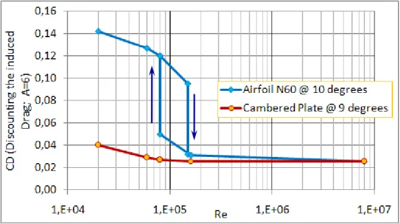
The transition zone is illustrated by figures 3.3 to 3.5, with values obtained from Hoerner (1958). In these figures the aerodynamic characteristics of two airfoils, presented in figure 3.6, are compared:
Cambered Plate 417a: T/C = 3.0%, Z/C =5.8% ; taken from chapter 6 of Hoerner (1958)
Figure 3.3: Variation of CL with Re for Cambered Plate and a Conventional Airfoil
Figure 3.5: Variation of L/D with Re for Cambered Plate and a Conventional Airfoil; values are consistent with the ones presented in figures 3.3 and 3.4
Figure 3.6: Cambered plate „417a‟ and airfoil N-60, from Schmitz (1942)
The very light aircraft Gossamer Condor and Solar Challenger of Paul MacCready, from about 70 to 80 years after, used airfoils with thickness about 12 to 14%, as can be seen in figure 3.7. According to Kroo and Alonso (2012) the Reynolds Number for airfoil „Lissaman 7769‟ of Gossamer Condor is about 500,000, and airfoil „Lissaman-Hibbs 8025‟ for Solar Challenger, is about 700,000 to 2000,000. Although special care was needed on the design of these 2 airfoils, they are above the Reynolds region of the abrupt reduction of L/D, presented in figure 3.5.
Figure 3.7: Airfoils from two aircraft designed by Paul MacCready; „Lissaman 7769‟ (above) for Gossamer Condor, and „Lissaman-Hibbs 8025‟ for Solar Challenger.
One interesting aspect related to low Reynolds number characteristics is that, according to Schmitz (1942) and Hoerner (1985), the strong reduction of the Lift-to-Drag ratio of conventional airfoils below 1.5x10⁵ presented in figure 3.5 was not commonly known; some tests performed at low Reynolds number (2x10⁴ to 2x10⁵) do not reproduce the effects of figure 3.5. The reason for this is that only tunnels of very low turbulence could be able to obtain these results. This effect of Lift-to-Drag ratio reduction occur due to laminar flow conditions; and the normal tunnels present a turbulence level in the test section that does not allow the flow to be laminar, as is the real free-stream flow condition during flight. Due to this, in some tests at these low Reynolds number levels, unrealistic and overoptimistic conclusions of airfoil behavior apparently occurred.
3.5.2) Variation of airfoil lift and drag coefficients with Reynolds number
the previous sub-section. It is an airfoil for airplane models in Germany by 1930. Besides its aerodynamic characteristics presented in NACA Report 628 (1938), its low-Reynolds characteristics have been obtained from the excellent work of Schmitz (1942). The second airfoil is the Eppler 387, which is an airfoil designed for low Reynolds Number, as presented in Selig et al (1989). According to Roland Boucher (2003) and Robert Boucher (1985), this airfoil is used on both aircraft Sunrise I and Sunrise II.
Figure 3.8: Airfoil N-60, T/C=12.4%; Z/C=3.8%, from NACA TN 388 (1931)
Figure 3.9: Airfoil Eppler 387, T/C~9%; Z/C~3.8%, from UIUC Airfoil Database.
a) Conventional airfoil „N-60‟ Lift and Drag Characteristics
Figure 3.10: 2-dimensional CL versus alpha for different Reynolds numbers, airfoil N-60
Figure 3.11: 2-dimensional CD versus alpha for different Reynolds numbers, airfoil N-60
An estimation of parameters Alph CLo, CLmax, CDo and K for the available Reynolds numbers have been performed based on the values and curves presented in figures 3.10 and 3-11. The values obtained for the coefficients are presented in figure 3.12, in function of Reynolds number.
0 0,2 0,4 0,6 0,8 1 1,2 1,4 1,6 1,8
-8 -6 -4 -2 0 2 4 6 8 10 12 14 16 18 20 22 24
C
L
2D
Alpha [degrees] Line of Max CL
CL Re [k] = 42 CL Re [k] = 63 CL Re [k] = 105 CL Re [k] = 3100
0 0,02 0,04 0,06 0,08 0,1 0,12
-8 -6 -4 -2 0 2 4 6 8 10 12 14 16 18 20 22 24
C
D
2
D
Alpha [degrees] CD Re [k] = 40
One can note that the factor K in this case represents the coefficient of the equation of the parabolic curve:
Being all the values CD, CDo, CL, referred to the curves of the (2-dimensional) airfoil drag and lift coefficients presented in figures 3.10 and 3.11.
Figure 3.12: Variation of N-60 airfoil 2-dimensional coefficients with Reynolds number
b) Eppler 387 Airfoil Lift and Drag Characteristics
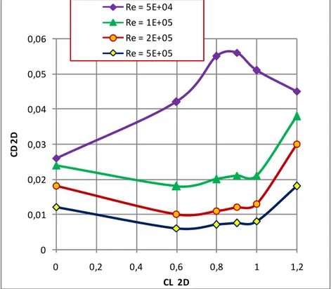
In order to define a variation of the drag with Reynolds Number for a good low-Reynolds number airfoil, the Eppler 387 characteristics are analyzed in this work, as presented in this sub-section. The airfoil main data, which is CD versus CL for several Reynolds Numbers are obtained from UIUC (2014), and presented in figure 3.13.
-8 -6 -4 -2 0 2 4 6
1,E+04 1,E+05 1,E+06 1,E+07
A
f C
L
, C
Lm
ax
, K
, C
D
o
Reynolds Number
As performed for N-60 airfoil in previous sub-section, parabolic curves of the type of equation 3.2are chosen to represent the airfoil CD versus CL curves presented in figure 3.13. The parabolic curves adopted are presented in figure 3.14. The coefficients CDo2D and K2D which define these curves are tabulated, in function of Reynolds number, for interpolation. The suffix 2D in the coefficients is to identify that they are related to the airfoil. The airfoil coefficients CDo2D and K2D obtained are presented as function of Reynolds number in figure 3.15.
The information of figure 3.15 is considered in this work, for the analysis of the aircraft drag, considering Reynolds effects. The values of airfoil lift, CLmax and αCLo, have been also obtained by the same procedure as the one performed for N-60 airfoil; and these values are shown as function of Reynolds number in figure 3.17, compared with the values of the same parameters for N-60 airfoil.
Figure 3.13: CD vs CL of Eppler 387 airfoil, for several Reynolds Numbers 0
0,01 0,02 0,03 0,04 0,05 0,06
0 0,2 0,4 0,6 0,8 1 1,2
C
D
2
D
CL 2D
Figure 3.14: Adjustment of Airfoil CD versus CL curves, for several Reynolds numbers
Figure 3.15: Coefficients CDo2D and K2D in function of Reynolds number 0
0,01 0,02 0,03 0,04 0,05 0,06
0 0,2 0,4 0,6 0,8 1 1,2
C
D
2
D
CL 2D
Re = 5,0E+05 Re = 2,0E+05 Re = 1,0E+05 Re = 5,0E+04
Adjusted for Re = 500000 Adjusted for Re = 200000 Adjusted for Re = 100000 Adjusted for Re = 50000
0,000 0,005 0,010 0,015 0,020 0,025 0,030 0,035 0,040
1,E+04 1,E+05 1,E+06
A
ir
fo
il
C
D
o
a
n
d
K
Reynolds Number
c) On comparing results of two airfoils
The values of CDo, K, αCLo and CLmax obtained for N-60 and Epller 387 airfoils are presented together in figures 3.16 and 3.17. In figure 3.16 the values of CDo and K for both airfoils are presented in function of Re, and in figure 3.17 the values of αCLo and CLmax for the two airfoils are presented, also as function of Reynolds number.
Figure 3.16: CDo and K versus Reynolds number for N-60 and Eppler 387 airfoils.
0 0,5 1 1,5 2 2,5 3 3,5 4 4,5 5
1,E+04 1,E+05 1,E+06 1,E+07
K
,
C
D
o
Reynolds Number
N-60 100*CDo N-60 10*K
Figure 3.17: αCLo and CLmax versus Reynolds number, for N-60 and Eppler 387 airfoils.
One can note that the hysteresis in the coefficients CDo and CLmax of N-60 airfoil are represented in figures 3.16 and 3.17. It is also evident from these two figures that both airfoil have their drag coefficient increased (by CDo comparison in figure 3.16) and the αCLo reduced (as shown in figure 3.16). Additionally it can be observed in these same figures that the Eppler 387 airfoil presents, for Re lower than 1.5E5, lower value of CDo and higher value of CLmax than the conventional airfoil N-60.
Through these comparisons it is possible to qualitatively show, how better is the Eppler 387 – or airfoils with similar shape – from more conventional airfoils of same camber, in the region of Reynolds number from 40,000 up to 150,000.
3.5.3) General Chart for Drag coefficients variation with Reynolds for non-cambered airfoils
One very useful tool for this research is the diagram of airfoil Drag coefficient versus airfoil Thickness ratio t/c and Reynolds number. This Diagram is presented in the figure 2, chapter 6, of Hoerner (1958). It is important to note that all airfoils of that figure are symmetrical.
-7 -6 -5 -4 -3 -2 -1 0 1 2
1,E+04 1,E+05 1,E+06 1,E+07
A
lp
h
C
Lo
[
de
gr
ee
s]
,
C
Lm
ax
Reynolds Number
N-60 alph CLo N-60 CL max
It is possible to superimpose the CDo values of Eppler 387 and N-60, presented in figure 3.5-11, to the above mentioned figure from Hoerner (1958). From this comparison, the most important points to observe is that the cambered airfoils Eppler 387 and N-60 presented an increasing in CDo roughly at the same Reynolds number range than the one presented for symmetrical airfoils; and that even in the regions with Re lower than 8x10⁴ as in regions with Re above 4x10⁵, the cambered airfoils presented a CDo significantly higher than the symmetrical airfoils with the same thickness.
Performing a rough analysis in these two regions (Reynolds number lower than 8 x 10⁴ as in regions with Reynolds number above 4 x 10⁵), by comparing the CDo of the two cambered airfoils with the CDo of the non-cambered ones with the same thickness ratio t/c at the same Reynolds number, it is possible to estimate the drag equivalence of delta Cdo due to camber as:
3.6) Literature Review of Solar Incidence Model
is the definition of several terms and concepts related to solar energy. But apparently, these models presented in these sources are destined to activities related to fixed points on Earth – such as satellite information check and solar power stations - in which the daily amount of solar energy is more important than the instantaneous solar power.
During the development of this work, soon it became evident that a self-sufficient model should be at least tried to be defined, for the purposes of solar aircraft research, since the model could be easier linked to the other tools. One additional stimulus to obtain a self-sufficient model is that this model could also be used for investigation of the sun-powered aerial navigation on other planets, as presented in Noth (2007, 2008e), proposing a Mars aerial vehicle and by Landis et al (2002) proposing a Venus aerial vehicle.
According to NASA (2014) the Sunlight power intensity - or irradiance - on the upper layer of atmosphere of Venus, Earth and Mars, are respectively 2613.9, 1367.6 and 589.2 W/m2 respectively. These values are the average, as the planets‟ distance to the sun suffers variation along the year. Considering the average distance to the Sun for the three planets, of 108.21, 149.60, and 227.92 all in magnitude of 106 km, it can be checked that the power intensity is consistent with the inverse of the square of the distance from the sun, which means that the reduction of the irradiance in the space between Sun and the planets is negligible.
3.7) Literature Review of Atmosphere
3.7.1) Earth‟s atmosphere
In terms of atmosphere, the most reliable information is the one found in NACA and ICAO (1954); ESDU (1986); and NOAA, NASA and USAF (1976).
The two most important parameters for the altitude flight analysis are air specific mass ρ and air kinematic viscosity ν. The air specific mass ρ can be obtained directly from the formulation presented in ESDU (1986). The kinematic viscosity ν is obtained from the dynamic viscosity µ and the air specific mass ρ, by:
The values of µ are obtained as function of the temperature, according to the relationship presented in Hoerner (1958). The variation of Temperature, ρ and ν with altitude, considered for this work, is presented in the figures 3.18 and 3.19.
Figure 3.18: Variation with altitude, of air absolute temperature
Figure 3.19: Variation with altitude, of air specific mass and kinematic viscosity
3.7.2) Sun irradiation and Earth‟s atmosphere 200 220 240 260 280 300
0 10 20 30 40 50
A ir T em pe ra tu re [ k] Altitude [km]
Temp [K]
Temp [K]0,00001 0,0001 0,001 0,01 0,1 1 10
0 10 20 30 40 50
A ir S pe ci fi c M as s [k g /m 3] an d Ki ne m at ic V is co si ty [ m 2/ s] Altitude [km]
Título do Gráfico Air Specific Mass [kg/m3]