Advances in Mechanical Engineering 2016, Vol. 8(5) 1–16
ÓThe Author(s) 2016 DOI: 10.1177/1687814016649110 aime.sagepub.com
Identification of modal parameters for
complex structures by experimental
modal analysis approach
Tamara Nestorovic´, Miroslav Trajkov and Matthias Patalong
Abstract
In this research, we have proposed a methodology for experimental identification of modal parameters based on mea-surement of the frequency responses of structures with complex geometries and performed an overall investigation of structural behavior on a funnel-shaped inlet of magnetic resonance tomograph. Several identification methods are imple-mented and compared: complex exponential, least-squares complex exponential, and polyreference least-squares com-plex exponential. We have implemented the modal parameter identification methodology within our own graphical user interface supported by MATLAB to create an independent tool for modal analysis. The estimation methods are com-pared and the comparison results are summarized showing based on tabular representation and stabilization diagrams significant advantage of the proposed methodology for determining eigenfrequencies, damping coefficients, mode shapes, and residues for complex structures investigated in broad band of frequencies. Runtime for the execution of algorithms vary depending on the applied method, assumed order of the model used for estimation, and the number of measure-ments, that is, inputs and outputs.
Keywords
Experimental modal analysis, identification of modal parameters, stabilization diagrams, frequency response functions, magnetic resonance tomograph funnel
Date received: 12 October 2015; accepted: 19 April 2016
Academic Editor: Francesco Massi
Introduction
Despite powerful simulation tools, modal analysis still remains an indispensable method for reliable investiga-tion of the structural behavior. Numerical structural models like the finite element (FE)-based ones can, in many cases, capture the structural behavior to a satis-factory extent of reliability, nevertheless some informa-tion might still be missing or cannot be accurately represented in such models. This is especially valid for material damping properties, which can still not be cap-tured accurately enough merely by a numeric simula-tion, where they can be implemented only as assumed values. Modal analysis can contribute to FE model improvement in such cases and it brings a number of
other advantages such as machine diagnosis, trouble-shooting problems, health monitoring, or other fields.
Development of tools which are used in estimation of modal parameters based on experimental measure-ments dates as early as development of some numerical algorithms, which were originally developed for solving
Mechanics of Adaptive Systems, Ruhr-Universita¨t Bochum, Bochum, Germany
Corresponding author:
Tamara Nestorovic´, Mechanics of Adaptive Systems, Ruhr-Universita¨t Bochum, Universita¨tsstr. 150, Building ICFW 03-725, D-44801 Bochum, Germany.
Email: [email protected]
some other problems.1Yet, a first major breakthrough in modal estimators appears with development of the maximum likelihood estimator in combination with the least-squares complex frequency domain estimator.2,3 An algorithm based on the polyreference least-squares estimator in the frequency domain has been proposed by Guillaume et al.4and Peeters et al.5Recently, Khader6 employed the unified matrix polynomial approach for modal parameter estimation. Previous works mainly consider just a single approach to identification of modal parameters. Regarding the implementation of the proposed algorithms, they are mainly applied on geome-trically simple structures, such as flexible beams.6–8In this article, we have proposed a procedure for modal parameter estimation which involves several modal esti-mation algorithms. In addition, we have tested not only our approach with geometrically simple structures (per-formed test example on the plate structure is here omitted, due to space limitation) but also the procedure with complex flexible three-dimensional (3D) shell struc-tures, like the funnel-shaped inlet of a magnetic reso-nance tomograph (MRT).
In implementation of the techniques for estimation of modal parameters based on measurement data, one is often confronted with requirement of using expensive commercial tools for modal analysis. Another arising problem is that usually standard techniques based on mere implementation of fast Fourier transform (FFT) are not satisfactory in determining modal parameters if even slight deviation from assumed linear properties of structures under consideration is present or if structures are not lightly damped. In such cases, it is very difficult, almost impossible to clearly distinguish the picks from the frequency response. To overcome these problems, we have contributed in this article a methodology for reliable estimation of modal parameters, which is based on conducting several steps, thorough out implementa-tion of required algorithms in order to determine modal parameters. We have developed our own tool, which is independent of any commercial platform for experi-mental modal analysis, and therefore represents a reli-able, but inexpensive, way for experimental modal analysis of demanding structures. Our further contribu-tion is development of a tool based on a MATLAB gra-phical user interface (GUI), which enables interactive manipulating of measurement data and implementation of parameter identification algorithms. The tool is advantageous for wide implementation in academia, research, and so on. Our modal parameter estimation methodology involves several estimation steps. The procedure begins with estimation of the mode indicator functions (MIFs). Subsequently, we have implemented, tested, and compared several modal parameter estima-tion algorithms. Due to limited space, we have pre-sented here only selected algorithms and investigation results, although different others are also included in
our tool (e.g. peak-picking method for estimation of the eigenfrequencies). Decision about relevant (resonant) frequencies is made based on stabilization diagrams, which are automatically generated as the output of our tool. Furthermore, detailed algorithms for complex exponential (CE), least-squares complex exponential (LSCE), polyreference least-squares complex exponen-tial (PRCE), and PRCE in frequency domain are pre-sented. The feasibility of the proposed methodology for the identification of the modal parameters of structures with complex geometries is documented on an example of a funnel-shaped structure, the inlet of the MRT. Obtained results include estimated eigenfrequencies, damping coefficients, and residues for different imple-mented algorithms. They are systematically represented by comparison tables and stabilization diagrams. In addition, the visualization of characteristic mode shapes of the funnel is presented.
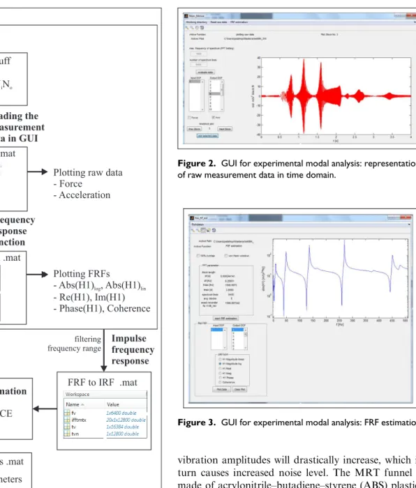
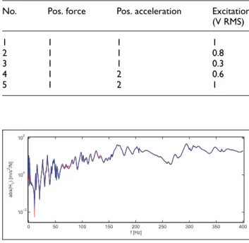
The funnel-shaped MRT inlet investigated in this article is characterized by complex geometry, and there-fore, the characterization of the modal parameters requires a careful investigation under implementation of the identification methods in order to produce reli-able statements about the eigenfrequencies, mode shapes, and damping coefficients. For that purpose, a detailed investigation was conducted in this article: sev-eral identification methods presented in Appendix 1 were implemented and their results were evaluated and compared. Experimental modal analysis is based on estimation of the frequency response functions (FRF) -the transfer functions between measured outputs and inputs of a structure, that is, on identification of modal parameters from the FRF. Complexity of the investi-gated structure can significantly influence the proce-dure for identification of its modal parameters. Due to lack or inaccessibility of some functionalities in avail-able commercial tools for experimental modal analysis, the authors of this article have developed their own tool for the identification of modal parameters based on the experimental measurement of the excitations and responses of structures and implemented it within a MATLAB-based GUI. Raw measurement data are read into GUI in universal file format. Required analy-ses are performed within GUI according to the execu-tion procedure shown in the chart of Figure 1. Corresponding results can be called and graphically represented in time and frequency domain, as shown by examples in Figures 2 and 3. In subsequent sections, the results of the tool implementation for the modal analysis of the MRT funnel inlet are presented.
Experimental determination of the MRT
funnel frequency responses
changing magnetic field, this diagnostic device is char-acterized by high noise emission, where the acoustic air pressure ranges from 60–100 dB and can therefore be very unpleasant, and if longer and frequently exposed, even harmful for the patients undergoing diagnostic treatment. If the frequency of a periodic excitation is close to one of the eigenfrequencies of the funnel, the
vibration amplitudes will drastically increase, which in turn causes increased noise level. The MRT funnel is made of acrylonitrile–butadiene–styrene (ABS) plastics and it weighs about 15 kg. To avoid strong resonant vibration and noise effects, active vibration control9–12 can be applied using piezoelectric actuator–sensor patches which are glued to the surface of the funnel and connected by cables via Bayonet Neill–Concelman (BNC) connectors with appropriate AD and DA con-verters. In addition, the funnel structure is reinforced by aluminum profiles attached to its back surface.
For efficient model-based active control, reliable modeling in early development phases before the con-troller design plays an important role. Modeling can be performed using numerical FE analysis.10,13,14Yet, it is often difficult and sometimes even not possible to pre-cisely model by the FE approach all important influ-ences like material properties of the funnel (especially damping properties), aluminum reinforcements, piezo-patches, and the cables, which have significant influence measurements .uff
measurements .mat
Reading the measurement data in GUI
fmax
Δt Nf
Main menu
N Ni o
Ndaten
Frequency response function
Plotting raw data - Force
- Acceleration
FRFs estimation .mat
Plotting FRFs - Abs(H1) , Abs(H1)
-- Coherence
log lin
Re(H1), Im(H1) Phase(H1),
windowing overlapping
FRF to IRF .mat
Impulse frequency response
filtering frequency range
Parameter estimation
- PP
- CE, LSCE, PRCE - PLSFD
Selection of modes
modal parameters .mat
modal parameters for corresponding degrees
of freedom All modal parameters
Figure 1. Flow chart of the frequency response and modal parameter identification implemented in GUI.
Figure 2. GUI for experimental modal analysis: representation of raw measurement data in time domain.
to modal parameters. Experimental modal analysis has therefore a great importance. FE models of the funnel including piezoelectric patches10,12–14are primarily used to determine from numerical modal analysis the critical eigenfrequencies, which are required in the controller design. In order to provide boundary conditions com-parable with the FE analysis, for the purpose of the experimental modal analysis, the funnel was hanged using four elastic springs, as shown in Figure 5. The cables with connectors—interface between the piezo-electric patches and AD–DA converters for the control purposes—are also hanged in such a way that they exert minimal or possibly no impact on the funnel.
Linearity test
In the linearity test, the funnel is excited at point 1 (Figure 5) using the shaker Bru¨el & Kjær (B&K) 4809.
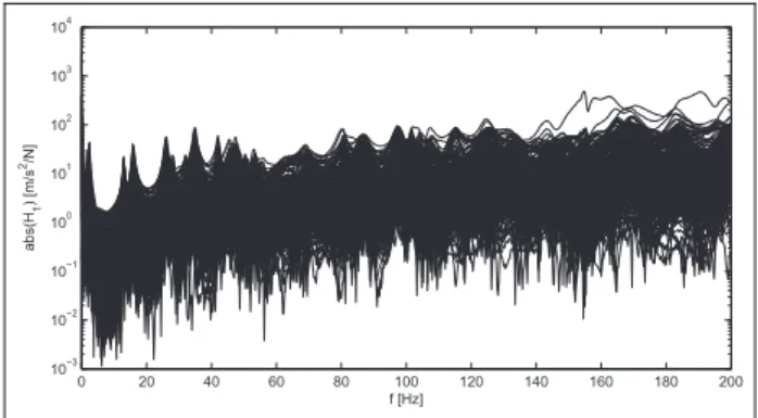
The force produced by the shaker is measured at the same point by the force transducer B&K 8230 placed at the top of the stinger connected with the shaker. The response of the funnel is measured by the one-dimensional (1D) accelerometer B&K 4507B at two dif-ferent positions (1 and 2 in Figure 5), according to Table 1. Measurements 1–3 are performed with acceler-ometer applied at drive point 1 (collocated with the shaker). Direction of the acceleration measurement at point 1 coincides with the excitation direction, which are in this case both vertical. Excitation is a pseudo random signal obtained through averaging of 10 blocks. Obtained frequency responses are shown in Figure 6 (also see Figure 7).
Measurements 4 and 5 are performed with acceler-ometer placed at position 2, further from the excitation Figure 4. MRT with funnel-shaped inlet (source: Siemens AG).
Figure 5. Experimental setup with the funnel hanged on four steel springs (positions 1 and 2 denote transducer positions).
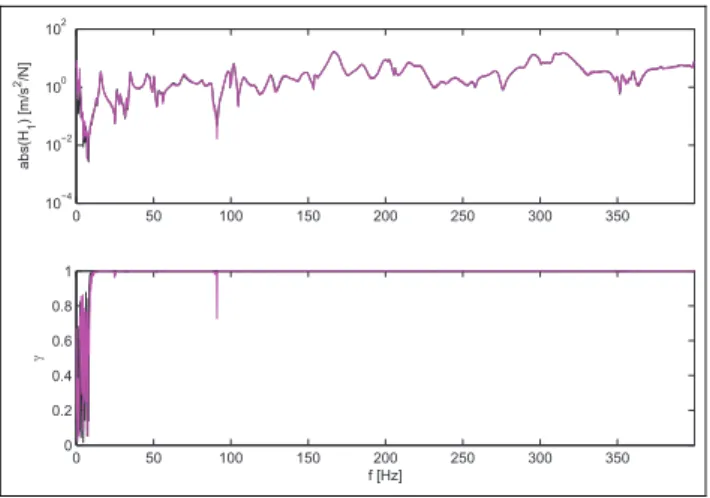
Table 1. Preview of measurements in the linearity test with transducer positions 1 and 2 (red in Figure 5).
No. Pos. force Pos. acceleration Excitation
(V RMS)
1 1 1 1
2 1 1 0.8
3 1 1 0.3
4 1 2 0.6
5 1 2 1
0 50 100 150 200 250 300 350 400
10−2 100 102
f [Hz]
abs(H
1
) [m/s
2/N]
Figure 6. Linearity test for the funnel: measurements 1–3, sensing at drive point. Measurements: 1 (black) 1.0 V RMS, 2 (red) 0.8 V RMS, and 3 (blue) 0.3 V RMS.
20 30 40 50 60 70 80 90 100
10−1 100 101
f [Hz]
abs(H
1
) [m/s
2/N]
point 1. Both the excitation and the response (accelera-tion measurement) direc(accelera-tions are vertical. Obtained fre-quency responses are represented in Figure 8. Good agreement can be observed. It should be noted that the signal level of the accelerometer for measurement 4 indicates a measurement under range. This can be avoided by increasing the excitation signal level to 1.0 V RMS, which improves the signal-to-noise ratio (Figure 9).
Single-input-multiple-output versus
multiple-input-multiple-output measurement and effect of the
accelerometer mass
In order to obtain complete overview of the structural behavior of the funnel, measurements of the structural response are performed in three perpendicular direc-tions using a 3D accelerometer. Single-input-multiple-output (SIMO) and multiple-input-multiple-Single-input-multiple-output
(MIMO) measurement cases were investigated in detail. Frequency responses for MIMOH1measurements were
performed according to Maia and Silva.15 Implementation of the MIMO measurement with two shakers with perpendicular directions of excitation could contribute on one hand to a uniformer energy distribution, supposedly excitation of all modes and lower signal levels, but on the other hand, it has resulted in lower partial coherence (correlation coeffi-cient, which describes possible causal relation between one output and all inputs12) about resonant frequen-cies. Therefore, for further investigations, a SIMO structural response measurement is performed using a rowing 3D accelerometer B&K 4524B in combination with the single shaker excitation. Due to adopted SIMO measurement procedure, only the investigation of the sensor mass effect could have relevance. The accelerometer used for the measurement has the mass which is approximately only 0.03% of the funnel mass, and therefore, it can be expected that it has a negligible influence to frequency response measurements. Comparison of the frequency responses for measure-ments 1 and 5 from Table 1 confirms this. For the first pronounced resonances, Figure 10 also confirms this, since only a negligible discrepancy between the reso-nant frequencies is present. Also, a classical test for investigation of the sensor mass influence, similarly as proposed in Baharin and Abdul Rahman,16has shown that the accelerometer mass can be neglected. Two fre-quency responses were measured, both with collocated input and output, but in the measurement of the second frequency response, additional sensor was applied at the neighboring degree of freedom, in this case ca. 10 cm from the drive point. Comparison of the fre-quency responses in Figure 11 shows that they are almost identical, which confirms that the influence of the sensor mass can be neglected.
Determination of the frequency responses
As described above, for the SIMO measurements, the force transducer B&K 8230 and the 3D accelerometer
0 50 100 150 200 250 300 350
10−4 10−2 100 102
abs(H
1
) [m/s
2/N]
0 50 100 150 200 250 300 350
0 0.2 0.4 0.6 0.8 1
f [Hz]
Figure 8. Linearity test for the funnel: measurements: 4 (black) and 5 (magenta); sensing far from excitation point.
0 20 40 60 80 100 120 140 160
100
abs(H
1
) [m/s
2/N]
0 20 40 60 80 100 120 140 160
0.9975 0.998 0.9985 0.999 0.9995 1
f [Hz]
Figure 9. Zoomed portion of Figure 8.
40 60 80 100 120 140 160 180 200
100
101
f [Hz]
abs(H
1
) [m/s
2/N]
B&K 4524B are used. In the frequency range up to 200 Hz, 800 spectral lines cover quite a large number of eigenfrequencies. The measurements are performed using B&K PULSE system, at predefined 107 points of the mesh represented in Figure 12, which define the positions of the 3D accelerometer. Since the transducer measures acceleration in three perpendicular directions, totally 321 measurement sets are obtained. Based on exported measurements, a diagram of the overlaid fre-quency responses with corresponding coherence (Figures 13 and 14) is created in MATLAB.
From Figures 13 and 14, it can be seen that first clearly separated eigenfrequencies appear in the fre-quency range up to 60 Hz. The range with bad coher-ence (under 10 Hz) is present due to shaker specification. Still it can be observed that bad coher-ence appears also for some frequencies above 10 Hz, but it occurs mainly at anti-resonant frequencies of
lower importance. At some frequencies below 5 Hz, double modes could be observed. They could represent either rigid body modes or elastic modes, but due to strong corruption by the measurement noise, the coher-ence corresponding to those modes is very bad and it does not allow a clear statement about them.
Identification of the MRT funnel modal
parameters
In order to identify the modal parameters of the funnel, a detailed analysis and comparison of several estima-tion methods presented in Appendix 1 has been per-formed. Main results of these investigations are presented subsequently. Due to space limitation, only selected results are represented by appropriate dia-grams or tables, others are explained and commented. Selected results of the implementation of methods for modal parameter identification are presented in terms of the stabilization diagrams.
Stabilization diagrams
Presented time-domain methods CE, LSCE, PRCE, and the polyreference least-squares complex frequency
0 50 100 150 200 250 300 350 400
10−2 100
102
abs(H
1
) [m/s
2/N]
f [Hz]
12 13 14 15 16 17 18 19
100
abs(H
1
) [m/s
2/N]
f [Hz]
Figure 11. SISO measurement test for investigation of the sensor mass influence. Black: measurement without neighboring additional sensor, magenta: measurement with additional sensor; below: zoomed portion.
Figure 12. PULSE model of the funnel with shaker and accelerometer positions; arrows represent measurement directions:x(red),y(blue), andz(black).
0 20 40 60 80 100 120 140 160 180 200
10−3 10−2 10−1 100 101 102 103 104
f [Hz]
abs(H
1
) [m/s
2/N]
Figure 13. Overlaid frequency responses of 321 measurement results for 107 points on the funnel with positions in Figure 12.
0 20 40 60 80 100 120 140 160 180 200
10−5
10−4
10−3
10−2
10−1
100
f [Hz]
abs(H
1
) [m/s
2/N]
domain (PLSFD) method are based on the assumed order n of underlying models. The order is related to calculated number of eigenfrequencies. Due to noisy measurement data, weak highly damped modes, or inexact model assumptions, the number of eigenfre-quenceis usually cannot be reliably determined based on measured frequency responses. If the number of modes is assumed to be higher than the actual number of modes, computational or fictitious modes will appear. Usual method which is used to distinguish between the real and the computational modes is based on repeated computation of the modes with one itera-tion over the ordern. If the estimated poles are plotted versus iterations, it can be noted that the real poles remain stable with regard to eigenfrequency, damping, and residues, whereas the computational modes are randomly scattered. In this way, the real poles can be selected by the user and kept for further processing. For models with high orders and high degrees of free-dom, the runtime can be large, depending on the algorithm.
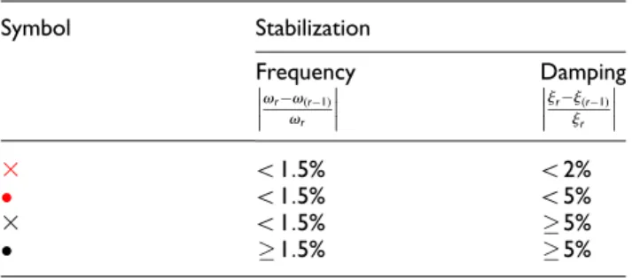
Table 2 represents four types of stable (Im(sr)\0)
underdamped poles. Unstable overdamped poles (jr.1) are not represented. Stabilization diagrams for
different estimation methods are represented for the magnetic resonance imaging (MRI) funnel inlet. The fourth type of poles from Table 2 (black dots) are not represented in diagrams, since they do not show stabili-zation and in addition for high orders of the modeln, the stabilization diagram would not be clearly represented.
Methods for identification of modal parameters
MIF1and CMIF mode indicator functions. MIF1and CMIF
(complex mode indicator function) mode indicator functions gave similar identification results. Due to negligible sensor mass effect, the methods allow SIMO measurement, but on the other hand, multiple eigenfre-quencies could not be identified. Significant lower eigenfrequencies can be clearly distinguished. Results for identified eigenfrequencies based on MIF1are pre-sented in a comparative tabular overview in section
‘‘Comparison of identified parameters.’’ Diagrams in Figure 15 represent the MIF1and CMIF mode indica-tor functions.
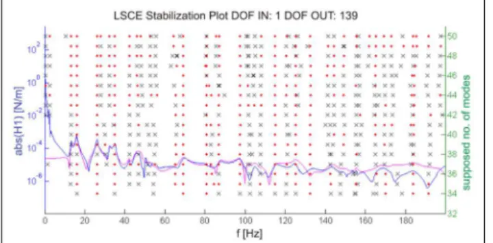
CE. CE method can identify most of the eigenfrequen-cies obtained from the mode indicator functions. Since some measurement points pertain to vibration nodes, not all eigenfrequencies in all frequency responses can be identified. The method performs fitting of a fre-quency response within entire range. In order to achieve appropriate pole stabilization, higher order for fitting has to be selected, which in turn may excite many unstable fictitious computational modes. Figure 16 rep-resents stabilization diagram for the frequency response 139.
LSCE. LSCE requires calculation of a pseudo inverse matrix, and it is therefore ineffective for large number Table 2. Criteria for poles in stabilization diagrams.
Symbol Stabilization
Frequency Damping
vrv(r1)
vr
jrj(r1)
jr
3 \1:5% \2%
\1:5% \5%
3 \1:5% 5%
1:5% 5%
0 20 40 60 80 100 120 140 160 180 200
0 0.2 0.4 0.6 0.8 1
MIF1
0 20 40 60 80 100 120 140 160 180 200
10−5
f [Hz]
CMIF
Figure 15. Mode indicator functions for the funnel.
0 20 40 60 80 100 120 140 160 180
10−6 10−4 10−2 100
abs(H1) [m/N]
CE Stabilisation Plot DOF IN:1 DOF OUT:139
0 20 40 60 80 100 120 140 160 180
10 20 30 40 50 60 70 80
supposed no. of modes
f [Hz]
of outputs. According to equation (13) in Appendix 1, for order n and number of outputs no, the pseudo
inverse of a (2nno)3(2n) matrix should be calculated.
In the case of the funnel, for no=321andn=50, this
matrix has dimension (32,100)3(100). Calculation of
the inverse matrix takes about 70 s. In some cases, lim-ited computer memory can influence the limitation of the selected order. Similarly, as with the method of CE, also here, the entire frequency range is used which requires increased orders to capture all frequencies, but in turn can invoke fictitious modes. The presence of fic-titious modes makes the selection of the poles more dif-ficult. Here, the LSCE has been implemented with order n=40,. . .,50. Mode indicator function MIF1
supports selection of poles in stabilization diagram. One representative result is shown in Figure 17.
PRCE. Implementation of this method takes ca. 65 s for one run with n=2,. . .,70. Stabilization diagram in
Figure 18 shows worse stabilization of the poles than for the CE and LSCE methods due to data inconsis-tency and due to the fact that the method was devel-oped for MIMO measurements. Determining the eigenfrequencies from the stabilization diagram is, therefore, in this case, not adequate.
Polyreference least-squares frequency domain. In order to show the advantages of the method without influence of data inconsistency, the properties of the method are first tested for a single-input-single-output (SISO) case. As a result, the stabilization diagram in Figure 19 is obtained. Frequencies lower than 10 Hz are excluded due to specification of the shaker which is responsible for low coherence in this range.
Due to properties of the method, it is also possible to set the upper limit for the investigated frequency range. In this way, the frequency responses can be well fitted even at higher frequencies with strongly coupled modes, without having to increase additionally the order of the method. This is shown exemplarily in Figure 20. Using this method, the frequency responses with strongly coupled and weak modes can be fitted well. Yet, implementation of the method to predefined narrow frequency ranges of SISO frequency responses in stabilization diagrams enables fitting of almost arbi-trarily weak peaks in the frequency response, which could result, for example, from measurement noise. In that way, almost any frequency response could be fitted. For example, the frequency close to 110 Hz in Figure 17. Frequency response 139: measured (blue) and
estimated using least-squares complex exponential (magenta).
0 20 40 60 80 100 120 140 160 180
10−6 10−4 10−2 100 102
abs(H
1
) [m/N]
PRCE Stabilization Plot DOF IN:1 DOF OUT:139
0 20 40 60 80 100 120 140 160 180
10 20 30 40 50 60 70
supposed no. of modes
f [Hz]
Figure 18. Frequency response 139: measured (blue) and estimated using PRCE (magenta).
20 40 60 80 100 120 140 160 180
10−6 10−5 10−4
abs(H
1
) [m/N]
20 40 60 80 100 120 140 160 180 20
40 60 80 100 120 140 160 180
n
f [Hz]
PLSFD Stabilization Plot DOF IN:1 DOF OUT:139
Figure 19. Frequency response 139: measured (blue) and estimated using SISO-PLSFD (magenta).
95 100 105 110 115
10−5
abs(H
1
) [m/N]
95 100 105 110 115
20 40 60 80 100 120 140 160 180
n
f [Hz]
PLSFD Stabilization Plot DOF IN:1 DOF OUT:139
Figure 20 identified by PLSFD could not be deter-mined using the mode indicator functions and it could originate from the measurement noise.
For the frequency range 10–120 Hz of the first 15 eigenfrequencies of interest, the stabilization is further improved, as Figure 21 for the SISO case shows.
Applied to SIMO data, this method significantly improves identification of global resonant frequencies (Figure 22), since in this case, information from all out-puts and for each frequency are used. The stabilization is especially good for the first eigenmodes with good consistency and small effect of the sensor mass, and clearly better than for the time-domain methods. Even by obvious increase in the method order n, less ficti-tious modes will be induced. In comparison with time-domain methods, PLSFD seems to also have a better robustness with respect to data inconsistency. Weak resonance at approximately 110 Hz in Figure 20 show-ing the SISO-PLSFD case appears also in stabilization diagram for the SIMO case (Figure 22), but no signifi-cant stabilization can be observed.
Computation of the PLSFD algorithm requires effi-cient programming in order to achieve fast runtime.
Matrices ½Xo and ½Yo in equation (32), Appendix 1,
should be calculated only once for high-model orders
n, since their order grows high with increasing number of inputs and spectral lines.5This is possible, since the matrices½Xoand½Yorepresent for small ordersnonly
submatrices of their larger versions. Time-consuming calculation of the left-hand side of the Kronecker prod-uct in both matrices of equation (32) should be per-formed only once. This submatrix can be saved and used twice, each time in½Xo and½Yo. Further runtime
savings could be achieved by calculation of this subma-trix using FFT,4 but in this work, we have not imple-mented this approach. Nevertheless, the computation is faster than with time-domain methods CE, LSCE, and PRCE.
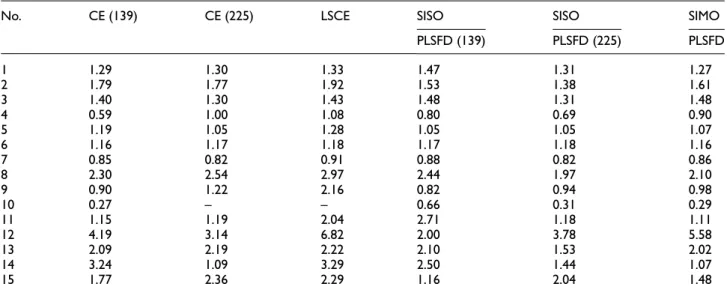
Comparison of identified parameters
Estimated modal parameters of the funnel are sented in Tables 3 and 4. Due to limited space, a repre-sentative frequency response 139 obtained by implementation of mentioned identification methods is shown on diagrams in the previous subsection. In addi-tion, for another frequency response, 225, the results are summarized in the tables for comparison purposes. Stabilization diagrams show, as expected, that SISO methods are not reliable to capture all eigenfrequenceis. However, SIMO methods— LSCE and PLSFD—are capable of a more reliable identification of all expected eigenmodes owing to larger data sets which capture information from all outputs. Eigenfrequencies are characterized by faster stabilization than the corre-sponding dampings.
Approximate runtime for the execution of the identi-fication algorithms is represented in Table 5. Among the implemented algorithms, SIMO-PLSFD shows best stabilization, runtime, and agreement of frequency responses. LSCE method is also characterized by accep-table stabilization, but it requires much more runtime.
Additional check of the results can be performed by animation of the vibration modes of the structure using appropriate software such as Labshop or PULSE. Multiple or rigid body modes can be distinguished through animation of the modes using imaginary parts of frequency responses as shown in Figure 23. For complex modes which exist in case of non-proportional damping, it is possible to perform the animation of modes using PULSE REFLEX software.
One drawback of the experimental modal analysis with used shaker B&K 4809 is caused by its specifica-tion of the measured frequency range, which results in bad coherence under 10 Hz and uncertain modal para-meter estimation in this range. In order to investigate this low-frequency region, another modal test has been performed, using impact hammer for excitation of the
20 30 40 50 60 70 80 90 100 110
10−5 10−4
abs(H
1
) [m/N]
PLSFD Stabilization Plot DOF IN:1 DOF OUT:139
20 30 40 50 60 70 80 90 100 110 20
40 60 80 100 120 140 160 180
n
f [Hz]
Figure 21. Frequency response 139: measured (blue) and estimated using SISO-PLSFD (magenta) in the frequency range 10–120 Hz.
20 30 40 50 60 70 80 90 100 110
10−7 10−6
10−5
10−4
10−3
abs(H
1
) [m/N]
PLSFD Stabilization Plot DOF IN:1 DOF OUT:139
20 30 40 50 60 70 80 90 100 110 20
40 60 80 100 120 140 160 180
n
f [Hz]
Table 3. Eigenfrequencies (Hz) based on MIF1and presented identification methods.
No. MIF1 CE (139) CE (225) LSCE SISO SISO SIMO
PLSFD (139) PLSFD (225) PLSFD
1 13 13.05 13.02 13.03 13.03 13.03 13.03
2 16 15.85 15.87 15.93 15.83 15.89 15.92
3 26 25.98 25.97 25.99 25.95 25.98 26.02
4 28 28.87 28.09 28.05 27.81 28.15 28.12
5 32.25 32.24 32.30 32.24 32.25 32.31 32.26
6 35 34.94 34.94 34.90 34.94 34.93 34.90
7 42.25 42.23 42.26 42.15 42.29 42.26 42.14
8 45.5 45.72 45.53 45.89 45.75 45.93 45.67
9 47.5 47.72 47.60 47.90 47.71 47.58 47.54
10 50.25 50.29 – – 50.32 50.13 50.34
11 53.25 53.39 53.24 52.53 52.54 53.02 53.06
12 64.25 63.46 63.16 64.28 63.35 66.71 64.98
13 69.25 69.17 69.27 69.04 69.18 69.16 69.07
14 80.75 80.23 81.20 80.71 80.07 80.42 80.99
85.25 85.11 85.34 85.44 86.92 85.18 87.00
MIF: mode indicator function; CE: complex exponential; LSCE: least-squares complex exponential; SISO: input-output; SIMO: single-input-multiple-output; PLSFD: polyreference least-squares complex frequency domain.
Table 4. Damping ratioj(in %) for corresponding eigenmodes of the funnel: comparison of different methods.
No. CE (139) CE (225) LSCE SISO SISO SIMO
PLSFD (139) PLSFD (225) PLSFD
1 1.29 1.30 1.33 1.47 1.31 1.27
2 1.79 1.77 1.92 1.53 1.38 1.61
3 1.40 1.30 1.43 1.48 1.31 1.48
4 0.59 1.00 1.08 0.80 0.69 0.90
5 1.19 1.05 1.28 1.05 1.05 1.07
6 1.16 1.17 1.18 1.17 1.18 1.16
7 0.85 0.82 0.91 0.88 0.82 0.86
8 2.30 2.54 2.97 2.44 1.97 2.10
9 0.90 1.22 2.16 0.82 0.94 0.98
10 0.27 – – 0.66 0.31 0.29
11 1.15 1.19 2.04 2.71 1.18 1.11
12 4.19 3.14 6.82 2.00 3.78 5.58
13 2.09 2.19 2.22 2.10 1.53 2.02
14 3.24 1.09 3.29 2.50 1.44 1.07
15 1.77 2.36 2.29 1.16 2.04 1.48
MIF: mode indicator function; CE: complex exponential; LSCE: least-squares complex exponential; SISO: input-output; SIMO: single-input-multiple-output; PLSFD: polyreference least-squares complex frequency domain.
Table 5. Approximate runtime for the algorithm execution on a Core2Duo E8400 4GB RAM computer.
Method (order) No. of FRFs Runtime (s)
CE (2–80)
LSCE (40–50)
PRCE (2–70)
PLSFD (10–150)
SISO 131 11 – – 7.6
SIMO 32131 321311 198 75 33
funnel. Frequency spectrum up to 100 Hz with resolu-tionDf =0,25Hz has been investigated.
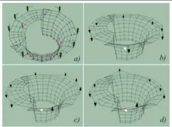
For excitation by the hammer, eight points on the funnel were predefined according to the mesh shown in Figure 24(a) (black: positions of the hammer). For out-put measurements, an accelerometer was glued by wax to the surface of the funnel. Red arrow in Figure 24(a) shows the position and measurement direction of the accelerometer. One frequency response with corre-sponding coherence is shown in Figure 25. Frequency responses show a good coherence. In this way, both
rigid body modes presented in Figure 24(b) and (c) could be distinguished. With their corresponding eigen-frequencies of 1.75 and 2.5 Hz, respectively, these two rigid body modes lay under 20% of the first elastic mode (Figure 24(d)) and have therefore a minimal effect on elastic modes. Furthermore, this investigation has confirmed the effectiveness of the funnel support by hanging it on springs, which simulates free body motion, similarly as assumed in the FE analysis. The rigid body modes are present due to supports and spring stiffness.
Conclusion
This article presents the identification of the modal parameters (eigenfrequencies, damping coefficients, residues, and mode shapes) based on measured FRF. Several time and frequency domain estimation algo-rithms are implemented within our MATLAB-based tool for the modal parameter estimation. An overall analysis of the structural behavior of the funnel-shaped inlet of MRT is performed based on the implemented estimation algorithms. The estimation methods are compared and the comparison results are summarized showing based on tabular representation and stabiliza-tion diagrams significant advantage of the proposed methodology for determining modal parameters in a broad band of frequencies.
Declaration of conflicting interests
The author(s) declared no potential conflicts of interest with respect to the research, authorship, and/or publication of this article.
Figure 23. Screen shots of the funnel eigenmodes obtained from the PULSE REFLEX animation.
Figure 24. (a) Mesh of the impact hammer test model. (b)–(d) Modes of the funnel obtained from PULSE: rigid body modes: first (b), second (c), and elastic mode (d).
Funding
The author(s) disclosed receipt of the following financial support for the research, authorship, and/or publication of this article: Article Processing Charge was funded partly by the German Research Foundation (Deutsche Forschungsgemeinschaft - DFG) and the Open Access Publication Fund of Ruhr-Universita¨t Bochum.
References
1. Prony R. Essai e´xperimental et analitique: sur les lois de la dilatabilite´ de fluides e´lastique et sur celles de la force expansive de la vapeur de l’Alkool, a` diffe´rentes tempera-tures.J Polytech1795; 1: 24–76.
2. Guillaume P, Verboven P and Vanlanduit S. Frequency-domain maximum likelihood identification of modal parameters with confidence intervals. In: Proceedings of the international conference on noise and vibration engi-neering (ISMA-23), Leuven, 16–18 September 1998. Leuven, Belgium: KU Leuven - Department of Mechani-cal Engineering.
3. El-Kafafy M and Guillaume P. Model parameter estima-tion of structures with over-damped poles. In:Proceeding of ISMA, Leuven, 2010, https://www.isma-isaac.be/past/ conf/isma2010/proceedings/papers/isma2010_0286.pdf 4. Guillaume P, Verboven P, Vanlanduit S, et al. A
poly-reference implementation of the least-squares complex frequency domain estimator. Proc IMAC 2003; 21: 183–192.
5. Peeters B, Van der Auweraer H, Guillaume P, et al. The PolyMAX frequency-domain method: a new standard for modal parameter estimation? Shock Vib 2004; 11: 395–409.
6. Khader N. Structural dynamic modification to predict modal parameters of multiple beams. In: Rossi M, Sasso M, Connesson N, et al. (eds)Residual stress, thermome-chanics & infrared imaging, hybrid techniques and inverse problems (Conference proceedings of the Society for Experimental Mechanics series, vol. 8). New York: Springer, 2013, pp.365–377.
7. Lee C-W and Kim J-S. Modal testing and suboptimal vibration control of flexible rotor bearing system by using a magnetic bearing. J Dyn Syst: T ASME 1992; 114: 244–252.
8. Ashory MR. High quality modal testing methods. PhD Thesis, Department of Mechanical Engineering, Imperial College of Science, Technology and Medicine, London, 1999.
9. Nestorovic´-Trajkov T, Ko¨ppe H and Gabbert U. Active vibration control using optimal LQ tracking system with additional dynamics.Int J Control2005; 78: 1182–1197. 10. Nestorovic´ Trajkov T, Ko¨ppe H and Gabbert U.
Vibra-tion control of a funnel-shaped shell structure with dis-tributed piezoelectric actuators and sensors.Smart Mater Struct2006; 15: 1119.
11. Nestorovic´ Trajkov T, Ko¨ppe H and Gabbert U. Direct model reference adaptive control (MRAC) design and simu-lation for the vibration suppression of piezoelectric smart structures.Commun Nonlinear Sci2008; 13: 1896–1909.
12. Oveisi A and Nestorovic´ T. Robust mixedH2/HNactive vibration controller in attenuation of smart beam.Facta Univ, Ser: Mech Eng2014; 12: 235–249.
13. Nestorovic´ T, Shabadi S, Marinkovic´ D, et al. Modeling of piezoelectric smart structures by implementation of a user defined shell finite element.Facta Univ, Ser: Mech Eng2013; 11: 1–12.
14. Nestorovic´ T, Marinkovic´ D, Shabadi S, et al. User defined finite element for modeling and analysis of active piezoelectric shell structures. Meccanica 2014; 49: 1763–1774.
15. Maia NMM and Silva JMM. Theoretical and experi-mental modal analysis. Baldock: Research Studies Press, 1997.
16. Baharin NH and Abdul Rahman R. Effect of acceler-ometer mass on thin plate vibration. J Mek 2009; 29: 100–111.
17. Allemang RJ and Brown DL. A complete review of the complex mode indicator function (CMIF) with applica-tions. In: Proceedings of ISMA international conference on noise and vibration engineering, Katholieke Universiteit Leuven, 2006, http://www.sdrl.uc.edu/sdrl/referenceinfo/ documents/papers/ISMA2006_CMIF.pdf
18. Brown DL, Allemang RJ, Zimmermann R, et al. Para-meter estimation techniques for modal analysis. SAE technical paper 790221, 1979.
19. Spitznogle FR and Quazi AH. Representation and analy-sis of time-limited signals using a complex exponential algorithm.J Acoust Soc Am1970; 47: 1150–1155. 20. Ewins DJ. Modal testing: theory, practice, and
applica-tion(Mechanical engineering research studies: engineer-ing dynamics series). Baldock: Research Studies Press, 2000.
21. Deblauwe F and Allemang RJ. The polyreference time-domain technique. In: Proceedings of the 10th interna-tional seminar on modal analysis, Part IV, Katholieke Universiteit Leuven, Leuven, 30 September–4 October 1985. Leuven, Belgium: KU Leuven - Department of Mechanical Engineering.
22. Cauberghe B.Applied frequency-domain system identifica-tion in the field of experimental and operaidentifica-tional modal analysis. Praca doktorska, VUB, Brussels, 2004.
Appendix 1
Methods for modal parameter identification
Mode indicator functions. Mode indicator function (MIF) is formulated to provide a tool for identifying closely spaced modes. Basic mathematical formulation of this indicator represents division of the real part of the FRF by its magnitude.
Mode indicator function MIF1implemented here is defined by equation (1). It can be used for single-input multiple-output (SIMO) measurements. For m sensor positions, it evaluates FRFs over all outputs. Hk(v)
MIF1(v) =
Pm
k=1
jReHk(v)j
2
Pm
k=1
jHk(v)j
2
ð1Þ
In this way, global modes become pronounced. Local modes cannot always be reliably estimated. Out of the resonant region, the function has value one or smaller than one. For a global resonance, the value of the function can drop to 0. As for other SIMO meth-ods, the modes which have nodes at or in the vicinity of the drive point cannot be identified.
Complex mode indicator function (CMIF) is based on a singular value decomposition (SVD) of the FRF matrix ½H(v) at each frequency. The requirement is that the number of inputs is smaller or equal to number of outputs. Singular values represent the contribution of each mode as a function of frequency. SVD is repre-sented by equation (2) where superscriptHdenotes the Hermitian matrix
H(v)
½ =½U(v)½S(v)½V(v)H ð2Þ Here, a modified form of the CMIF17is implemented, in which only the imaginary partIm½H(v)of the FRF matrix is used. The singular values, that is, the diagonal values of the matrix½S(v) are calculated. This results in clearly distinguished closely spaced modes. Ascending singular values are represented in logarith-mic scale. The peaks represent resonant frequencies. If two adjacent singular values correspond to the same resonant frequency, a double mode can be expected in the neighborhood of the corresponding spectral line. Nonlinearities, effect of the sensor mass, or measure-ment noise can lead to unclear indicator functions or even to fictitious computational modes.
Complex exponential. The complex exponential (CE) method belongs to time-domain identification methods, in which modal parameters are estimated based on the impulse response of a structure.15,18,19 It assumes that investigated structure can be represented as a linear vis-cously dampedndegree-of-freedom system. Frequency response is defined based on the receptance function
Hjk(displacement at pointjdue to a force at pointk)
Hjk(v) = P
2n
r=1
rAjk
vrjr+i(vv0r)
v0r=vr
ffiffiffiffiffiffiffiffiffiffiffiffiffi
1j2
r q
,v0r+n= v0r,(r+n)Ajk=rAjk
ð3Þ
wherevrrepresents the natural frequency,jr is the
vis-cous damping factor,rAjk is the residue corresponding
to each moder, andrepresents the complex conjugate. Impulse response equation (4) ofHjk as a function of
time can be obtained by applying the inverse Fourier transform to equation (3)
hjk(t) = X
2n
r=1
rAjkesrt,sr=vrjr+iv0r ð4Þ
Within considered time frame q, discretized at equally spaced time intervals Dt=1=Df, the impulse response is represented as a discrete-time series
h0,h1,h2,. . .,hq=h(0),h(Dt),h(2Dt),. . .,h(qDt) ð5Þ
With abbreviations rAjk=Ar and esrDt=Vr
intro-duced in equation (4), one can write for the lth time instant
hl= X
2n
r=1
ArVrl ð6Þ
whereltakes values from 0 toq, and therefore equation (6) can be written in developed form as a set ofq+1
equations, one corresponding to each time instant. Both Ar and Vr are unknown. They are determined
using Prony’s1method. The idea behind this method is that since the poles of the underdamped system always appear as complex conjugate pairs, this will also be valid for the modified variables Vr. If the number of
measurements is greater than4n, with equation (6), an
eigenvalue problem can be created, the solutionsVr of
which contain the poles of the structure. Thus, there always exists a polynomial of order qin Vr with real
coefficientsb (autoregressive coefficients), so that rela-tion equarela-tion (7) is valid
b0+b1V+b2V 2
+ +bqVq=0 ð7Þ
Several transformations15 lead to a set of equations in matrix form equation (8), from which the coefficients
bcan be obtained
h
½
(2n32n)
fbg
(2n31)
= f~hg
(2n31)
ð8Þ
Substituting the b coefficients in equation (7) and calculating the corresponding polynomial roots, the val-ues ofV1,V2,. . .,V2n can be determined. The poles sr
are obtained from
Vr=esrDt ð9Þ
Set ofq+1equation (6) in developed form can be
written shorter as a matrix equation
V
½ fAg=fhg ð10Þ which can then be solved for residuesfAg=½V1fhg.
depends on the selected order q of the polynomial in equation (7). Forq=2n, according to theoretical
back-grounds for small viscous damping,15,20 as a result n
pairs of complex conjugate poles should be expected. In practice, calculation with non-ideal data sets may result besides complex conjugate, also in unstable (Re(sr).0) or overdamped (Im(sr) =0) poles. They
must be excluded from the set of polessr. Overdamped
poles can be recognized byIm(Vr) =0, and they can be
removed from fVgbefore implementation of equation (9). For calculation of modal constants in fAg, entire matrix fVg(2n31) including unstable modes must be
used. Indices of removed poles can be saved and corre-sponding modal constants with same indices as removed poles can be removed from fAg. In this way, only underdamped and stable pole pairs and their cor-responding modal constants are retained for further calculation.
Least-squares complex exponential. Least-squares complex exponential (LSCE) method represents a modification of the CE method, so that it can be extended to SIMO measurements.15In this case, a set of impulse responses is used, where one input excites poutputs. In compari-son with CE, LSCE results in a more consistent model, without variation of parameters over outputs. Considerable computational savings can be achieved by the unique selection of the eigenfrequencies. Since the b coefficients represent global values, equation (8) can be extended to all outputs
h
½ 1
h
½ 2 .. .
h
½ p
2
6 6 6 4
3
7 7 7 5
fbg= f~hg1
f~hg2 .. .
f~hgp
8
> > > <
> > > :
9
> > > =
> > > ;
ð11Þ
or in shorter matrix form
hG
½
(2np32n)
fbg
(2n31)
= f~h
Gg (2np31)
ð12Þ
Least-squares solution for the b coefficients can be determined by calculation of a pseudo inverse
fbg= ½hGT½hG
1
hG
½ Tf~h
Gg ð13Þ
or in MATLAB using function pinv(). With deter-minedfbgmatrix of coefficients,fVgcan be calculated from equation (7). For each output i, matrixfAgi can be determined from equation (10) using corresponding vectorfhgifor theith output.
Polyreference least-squares complex exponential. Polyreference least-squares complex exponential (PRCE) method represents extension of the LSCE
method to multiple-input-multiple-output (MIMO) case.21It results in a consistent model of large, lightly damped structures. Since several inputs are used, it is less likely that the drive point will be set at some of the vibration nodes. The modal constants (residues)rAjkof
the impulse response in equation (4) are for each mode
rproportional to elements of the eigenvectorsfCgby a scaling factorQr
rAjk=QrCjrCkr ð14Þ
Thus, the residue of the rth mode atjth output due to excitation at first input will be
rAj1=QrCjrC1r ð15Þ
With modal participation, vectorrWk1can be defined
as
rWk1=
Ckr
C1r
ð16Þ
the residue for thekth output becomes
rAjk=rWk1rAj1 ð17Þ
Taking into account equation (4) and considering q
inputs, the impulse response at outputjcan be written in matrix form as
fhj(t)g=½ W
es1t 0 . . . 0 0 es2t . . . 0
.. .
.. .
. . .
.. .
0 0 . . . es2nt 2
6 6 4
3
7 7 5
fAj1g ð18Þ
where½Wrepresents the modal participation matrix. If the impulse response is discretized atL+1equidistant
points (sampling time Dt), a set ofL+1matrix
equa-tions can be written
fhj(iDt)g=½ W ½ V ifAj1g,i=0,. . .,L ð19Þ
where
V
½ =diagfes1Dt
,es2Dt
,. . .,es2nDtg ð20Þ
Similarly, as with the CE and LSCE methods, the2n
eigenvalues of the system are determined as roots of the matrix polynomial
XL
k=0 bk
½ ½ W ½ V k=0 ð21Þ
where ½bk represents the real quadratic matrices of coefficients with order q (number of inputs). Matrix polynomial equation (21) will have 2nroots (i.e.
the coefficients matrix is equal to2n, that is,2n=Lq.
The number of samplesLof the impulse response must therefore be at least2n=q. IfL.2n=q, then the fictitious
or computational modes will appear. Later, they can be recognized as unstable poles in the stabilization dia-grams or as too high damping coefficients and can be removed. In order to determine the coefficient matrices ½bk, theL+1equations in equation (19) are multiplied
by½b0, . . .,½bL, respectively, and they are afterwards
added together. Since taking into account (21), the right-hand side of the obtained sum is equal to 0, then also the left-hand side must be equal to 0
XL
k=0 bk
½ fhj(kDt)g=f0g ð22Þ
Through further transformations,15 the eigenvalues
Vr are determined by finding numerical solution of the
eigenvalue problem written in the form of companion matrix equation. Using equation (9) andVr, the poles,
that is, eigenfrequencies and damping factors can be determined. From the eigenvalue problem in the form of companion matrix equation, the eigenvectors can be determined, which containfz0g=fWrg, thus the modal
participation matrix ½W is also determined and it remains to calculate the residues. They can be obtained from equation (19) by varying the indexi, which results in
fhj(0)g
fhj(Dt)g
.. .
fhj(LDt)g 8 > > > < > > > : 9 > > > = > > > ; = W
½ ½ V 0 W
½ ½ V 1
.. .
W
½ ½ V L
2 6 6 6 4 3 7 7 7 5
fAj1g ð23Þ
or shorter in matrix form fHjg ((L+1)q31)
= ½WV ((L+1)q32n)
fAj1g
(2n31)
ð24Þ
From equation (24), the residues can be calculated as
fAj1g= ½WVH½WV
1
WV
½ HfHjg ð25Þ
where superscriptH denotes the Hermitian transpose. The calculation in equation (25) is repeated for all out-puts j=1,. . .,p. When all fAj1g are known, all
resi-dues can be determined from equation (17).
Polyreference least-squares complex frequency domain. The polyreference least-squares complex frequency domain (PLSFD) method has been developed for MIMO dis-placement frequency responses.2,4 It is also known as PolyMAX method.5 Here, we implement a weighted version, in which the frequency-dependent coherence is
used as a weighting of the output degrees of freedom.4,22
The frequency response matrix½H(v) is subdivided with respect to outputsNi. The influence of each output
Ni can be formulated using the right matrix fraction
description (RMFD). For theoth output, the influence of all inputs can be formulated as
^
Ho
=½No(v)½ D(v)
1
ð26Þ with the numerator row-vector polynomial
No
½ (v)2C13Ni
No
½ (v) = X
n
j=0
Oj(v) Boj
ð27Þ
and denominator matrix polynomial½ D(v)2CNi3Ni
D(v)
½ =X
n
j=0
Oj(v) Aj
ð28Þ
Symbol^in equation (26) denotes the estimated model-based frequency responses (not from measure-ments). Coefficients ½Aj und ½Boj are the parameters
to be determined. They can be arranged within the matrix
u
½ = ½b1
T,. . .,
bNo
T
,½ aT
h iT
ð29Þ where
bo
½ =
Bo0
½
Bo1
½ .. . Bon ½ 8 > > > < > > > : 9 > > > = > > > ;
, o=1,. . .,N0; ½ a =
A0 ½ A1 ½ .. . An ½ 8 > > > < > > > : 9 > > > = > > > ;
ð30Þ Scalarnrepresents the order of the model, and it is varied to generate the stabilization diagrams. The para-meter estimation problem is solved by minimizing the cost function with respect tou, which corresponds to solving the linearized minimization problem resulting in4,22
Re J H
J
½
½ u =½ 0 ð31Þ
where½Jrepresents the Jacobian matrix
J
½ =
X1
½ 0 0 ½ Y1
0 ½X2 0 ½ Y2
.. . . . . .. . .. .
0 0 . . . XN o
½ ½YNo 2 6 6 6 4 3 7 7 7 5
ð32Þ
The matrices ½Xo, ½Yo, o=1,. . .,No in equation
and frequency-dependent weighting functions Wo(vf).5
With determined ½a and ½bo from the optimization
problem, the poles and modal participation factors can now be obtained as the eigenvalues and eigenvectors of the companion matrix
Ac=
A0n1
A0n2
. . . A01
A00
INi
½ ½ 0 . . . ½ 0 ½ 0
0
½ .. . . ½ 0 ½ 0
.. . .. . . . . .. . .. . 0
½ ½ 0 . . . IN i
½ ½ 0 2 6 6 6 6 6 6 4 3 7 7 7 7 7 7 5
ð33Þ
where
A0j
h i
= ½An
1
Aj
= ½INi
1
Aj
= Aj
ð34Þ Submatrices ½Aj correspond to equation (30), and
they are extracted accordingly in the procedure of determining ½a.3,4 The poles lr are obtained as the
eigenvalues of the companion matrix ½Ac. The modal
participation factors are the lastNi rows of the matrix
of eigenvectors ½V 2CnNi3nNi in equation (33). The
residuesrAjk,rAjk, that is, the mode shapes are obtained
in the subsequent step. For that purpose,½H^is written
in the form of equation (35) using additional residues ½UR and½LR, which model the influence of the upper and lower modes, respectively, outside of the consid-ered frequency range. Their influence may be especially strong, if the band limit frequencies are slightly higher or slightly lower than the frequencies of the modes which are not clearly distinguished, but which must not be neglected. The effect of these terms can be clearly distinguished if the measured and the estimated fre-quency responses are overlaid
^
H
(v) = X
2n
r=1
rA
½
jvsr
+ rA ½
jvs
r
+ ½LR
(jv)2 +½UR ð35Þ
Direct solving of equation (35) does not guarantee the assumed complex conjugate residues ½rAand½rA. In order to overcome this problem, in this step, the damping can be approximated with often more realistic assumption of hysteresis damping coefficientshr’2j
r.
Then, equation (35) can be written as
^
Hik(v) =
Xn
r=1
rAik rv2v2+jhr rv
2
+ LRik
(jv)2 +URik ð36Þ Linear least-squares approximation of equation (36) written for Nf frequencies results in the following
matrix form
HV
½
(Nf31)
= ½PM (Nf3(n+2))
½AV ((n+2)31)
ð37Þ
where
fHVg=
Hik(v1)
Hik(v2)
.. .
Hik(vNf)
8 > > > < > > > : 9 > > > = > > > ;
, fAVg=
1Aik
.. .
nAik
LRik URik 8 > > > > > < > > > > > : 9 > > > > > = > > > > > ; , PM
½ =
1
1v2v21+jh1 1v 2
1
nv2v21+jhn nv 2
1
(jv1) 2 1 1
1v2v22+jh1 1v2
1
nv2v22+jhn nv2
1
(jv2) 2 1 .. . .. . .. . .. . .. . 1
1v2v2
Nf+jh1 1v2
1
nv2v2Nf+jhn nv2
1
(jvNf)2 1
2 6 6 6 6 6 4 3 7 7 7 7 7 5
Least-squares approximation of fAVg is then
obtained as
fALSV g= ½PMH½PM
1
PM