Padrão sazonal da produção industrial, exportações e importações: uma aplicação do X-12 ARIMA

(1)

EAESP/FGV/NPP - N

ÚCLEODE

P

ESQUISAS E

P

UBLICAÇÕES

1/96

RE L A T Ó R I O D E PE S Q U I S A Nº 1 6 / 1 9 9 8

RESUMO

Este trabalho tem por objetivo identificar os coeficientes sazonais de algumas

variáveis econômicas (produção industrial, exportações e importações), isentos das

mudanças estruturais registradas na economia. O estudo verifica se os planos de

estabilização implementados pelo governo nos últimos quinze anos afetaram o

padrão sazonal daquelas séries.

Para tanto aplica-se o X-12-ARIMA, o novo método de dessazonalização de séries

desenvolvido pelo U.S. Bureau of the Census. O uso desse método torna-se

necessário, porque os demais métodos conhecidos impedem testar nossa hipótese, ao

não permitirem o emprego de intervenções, não obtendo assim os melhores

estimadores para os coeficientes sazonais.

O estudo cobre o período que vai de 1980 a 1997 e os resultados confirmam a nossa

hipótese de mudança no padrão sazonal no período.

As nossas variáveis econômicas foram - de um ou de outro modo - atingidas pelos

planos de estabilização implementados nos últimos quinze anos.

PALAVRAS-CHAVE

Sazonalidade; X-11-ARIMA; X-12-ARIMA.

ABSTRACT

(2)

EAESP/FGV/NPP - N

ÚCLEODE

P

ESQUISAS E

P

UBLICAÇÕES

2/96

govern over the last fifteen years affected the seasonal pattern of our economic time

series.

In order to do that, the X-12-ARIMA, the new method to adjust time series for

seasonal effects developed by the U.S. Bureau of the Census, will be used. The use

of this new method it is necessary because, if our hypothesis is true, the standard

methods employed to adjust Brazilian time series for seasonal effects may fail in

obtaining the best estimators for the seasonal coefficients. The X-12-ARIMA is a

method which filters the time series allowing for corrective interventions.

The study covers the period from 1980 to 1997 and the results confirm the

hypothesis of changes in the seasonal coefficients during this period.

KEY WORDS

(3)

EAESP/FGV/NPP - N

ÚCLEODE

P

ESQUISAS E

P

UBLICAÇÕES

3/96

SUMÁRIO

I. Introdução ... 4

II. O método X-12-ARIMA: um rápido panorama. ... 5

III. As variáveis econômicas objeto de estudo ... 9

IV. Resultados

da

pesquisa ... 12

1. Introdução ... 12

2. Indústria de Transformação ... 14

2.1. Efeitos da composição do mês ... 14

2.2. Efeitos dos dias úteis trabalhados ... 20

3. Importações ... 24

3.1. Efeitos da composição do mês ... 24

3.2. Efeitos dos dias úteis trabalhados ... 29

4. Exportações ... 34

4.1. Efeitos da composição do mês ... 34

4.2. Efeitos dos dias úteis trabalhados ... 39

V. Conclusão ... 44

VI. Bibliografia ... 45

(4)

EAESP/FGV/NPP - N

ÚCLEODE

P

ESQUISAS E

P

UBLICAÇÕES

4/96

PADRÃO SAZONAL DA PRODUÇÃO INDUSTRIAL,

EXPORTAÇÕES E IMPORTAÇÕES: UMA

APLICAÇÃO DO X-12-ARIMA

Arício Xavier de Oliveira*

I. INTRODUÇÃO

A economia brasileira foi submetida desde o ano de 1986 a sucessivos planos de

estabilização. Para os estudiosos da conjuntura - aqueles que tentam entender e

explicar os movimentos de curto prazo das variáveis econômicas - a conseqüência

daqueles planos foi muitas vezes modificar a estrutura das séries de tempo,

dificultando ou falseando a análise. Porém as conseqüência não ficam apenas para

quem estuda a conjuntura, mas alcança também a quem executa a política

econômica, que deveria se orientar por indicadores conjunturais confiáveis. O

problema, em última análise, deve-se a que a análise conjuntural faz uso de

componentes não observados (tendência, ciclo, sazonalidade), extraídos das séries

temporais segundo métodos estatísticos, que nem sempre conseguem isolá-los

adequadamente.

O que falta a tais métodos ? Os distúrbios que surgem nas variáveis econômicas, em

conseqüência dos planos de estabilização - e não somente por esses planos (que

fique bem claro) - são quebras estruturais, mudanças na tendência, etc, traduzidas

em alterações no nível das séries, na sua inclinação, etc. Logo, o método de

decomposição de séries que permita tratar esses fenômenos pode produzir uma

melhor informação que os demais.

(5)

EAESP/FGV/NPP - N

ÚCLEODE

P

ESQUISAS E

P

UBLICAÇÕES

5/96

Os métodos de extração do componente sazonal conhecidos até hoje - ou até o

surgimento do 12 - desde o clássico de médias móveis, passando pelo Census

X-11 e outros menos referidos, chegando finalmente ao X-X-11-ARIMA de Estela

Dagum, não propiciam recursos e/ou flexibilidade para incorporar os fenômenos

descritos. A grande contribuição do X-12-ARIMA, a nosso ver, foi justamente

preencher essa lacuna, ao incorporar conceitos da técnica de análise de intervenção

na pré-filtragem das séries, como veremos adiante.

II. O MÉTODO X-12-ARIMA: UM RÁPIDO PANORAMA

O X-12-ARIMA é uma evolução direta do X-11-ARIMA do Canadá ou de Estela

Dagum, como é conhecido. As suas principais características e avanços estão

descritos em Findley et alii (1996), praticamente a única bibliografia existente a

respeito. O diagrama mostrado a seguir consta na página 3 de Findley et alii (1996)

e é bastante elucidativo:

X-12-ARIMA

RegARIMA Models

(Forecasts, Backcasts,

Preadjustments)

Modeling and Model

Comparison Diagnostics

SEASONAL ADJUSTMENT

(Enhanced X-11)

(6)

EAESP/FGV/NPP - N

ÚCLEODE

P

ESQUISAS E

P

UBLICAÇÕES

6/96

Os avanços do X-12-ARIMA se deram nos vários módulos mostrados no diagrama

anterior, mas principalmente pela inclusão do RegARIMA, um programa já

existente no U.S. Bureau of the Census, que foi renovado e introduzido aqui como

uma rotina preliminar ao ajustamento sazonal propriamente dito, o qual é realizado

no âmbito do X-12-ARIMA com as técnicas (melhoradas) do X-11-ARIMA. O

RegARIMA permite uma série de ajustes prévios, que vão desde a correção por dias

úteis, anos bissextos, variáveis definidas pelo usuário (que assim pode introduzir

características locais), até à identificação automática e estimação simultânea de

“outliers” (tipos AO, LS, TC) (vide Chen et alii, 1990). A filtragem inicial

realiza-se quarealiza-se que mediante uma função de transferência, excetuando-realiza-se o fato de que o

RegARIMA não permite a especificação de denominadores nas variáveis de entrada.

A identificação dos ARIMAS realiza-se com o instrumental conhecido, a função de

autocorrelação e a função de autocorrelação parcial. É nessa fase - a do RegARIMA

- que são identificadas as eventuais mudanças significativas na estrutura das séries

de tempo, se elas foram ou não incorporadas pelo processo gerador das séries. Se

não o foram, são “denunciadas” em sua maioria pela presença de “outliers”, que

deverão estar associados em geral a eventos econômicos conhecidos.

Somente depois de submetida a esses filtros, que eliminam componentes

identificáveis e que nada têm a ver com a sazonalidade, é que a série temporal é

submetida ao módulo seguinte, um X-11 melhorado.

Usando a notação de Findley et alii (1996), já usual na literatura de séries de tempo

(vide Box, Jenkins and Reinsel, 1994), a fase do RegARIMA ficaria assim:

φ

p

(B)

Φ

P

(B

s

) (1 – B)

d

(1 – B

s

)

D

(Y

t

-

Σβ

i

X

it

) =

θ

q

(B)

Θ

Q

(B

s

)a

t

,

i = 1 até r

.

(7)

EAESP/FGV/NPP - N

ÚCLEODE

P

ESQUISAS E

P

UBLICAÇÕES

7/96

cumprir as propriedades de estacionariedade, invertibilidade, normalidade dos erros

e variância constante.

Depois dessa etapa inicial e decisiva de filtragem da série - e que caracteriza o X-12

- seguem-se os procedimentos de decomposição e extração do componente sazonal,

minuciosamente descrito em Findley et alii (1996), cuja discussão não é objeto

dessa pesquisa.

O que apresentamos a seguir é o esquema de decomposição de séries multiplicativas

- a melhor alternativa identificada para as séries em estudo - uma transcrição parcial

do citado trabalho de Findley et alii (1996):

PROCEDIMENTOS DO X-11 PARA A DECOMPOSIÇÃO DE SÉRIES DE

TEMPO

Supondo que Y

t

= T

t .

S

t .

I

t .

Sendo T

t

= tendência, S

t

= sazonalidade e I

t

= irregularidades, uma série temporal

mensal sem “outliers” Y

t

, pode ser assim decomposta:

Estágio 1 (estimativas iniciais)

(i) Tendência inicial estimada:

T

t (1)

= (1/24)Y

t-6

+ (1/12)Y

t-5

+...+ (1/12)Y

t

+...+ (1/12)Y

t+5

+ (1/24)Y

t+6

(ii) Razão SI inicial:

SI

t (1)

= Y

t

/ T

t (1)

(8)

EAESP/FGV/NPP - N

ÚCLEODE

P

ESQUISAS E

P

UBLICAÇÕES

8/96

(iii) Fator sazonal inicial via média móvel sazonal “3 x 3”:

S^

t(1)

= (1/9)SI

(1)t-24

+ (2/9)SI

(1)t-12

+ (3/9)SI

(1)t

+ (2/9)SI

(1)t+12

+ (1/9)SI

(1)t+24

,

onde S^= S calculado

(iv) Fator sazonal inicial:

S

(1)t

= S^

(1)

t

/ (1/24)S^

(1)

t-6

+ (1/12)S^

(1)

t-5

+...+ (1/12)S^

(1)

t+5

+ (1/24)S^

(1)

t+6

,

onde S^= S calculado.

(v) Ajustamento sazonal inicial: A

(1)t

= Y

t

/ S

(1)

t

Estágio 2 (fatores sazonais e ajustamento sazonal)

(i) Tendência intermediária:

T

(2)t

=

Σ

h

j (2H+1)

A

(1)t+j

, j=-H até H, onde H=pesos de

Henderson

(ii) SI

(2)t

= Y

t

/ T

(2)t

(iii) Fator sazonal preliminar via média móvel sazonal “3 x 5” :

S^

(2)t

= (1/15)SI

(2)

t-36

+ (2/15)SI

(2)

t-24

+ (3/15)SI

(2)

t-12

+ (3/15)SI

(2)

t

+

(3/15)SI

(2)t+12

+ (2/15)SI

(2)

t+24

+(1/15)SI

(2)

t+36

(iv) Fator sazonal :

S

(2)t

= S^

(2)

t

/ (1/24)S^

(2)

t-6

+ (1/12)S^

(2)

t-5

+...+ (1/12)S^

(2)

t+5

+ (1/24)S^

(2)

t+6

(v) Ajustamento sazonal : A

(2)t

= Y

t

/ S

(2)

(9)

EAESP/FGV/NPP - N

ÚCLEODE

P

ESQUISAS E

P

UBLICAÇÕES

9/96

Estágio 3 (Estimativa final da tendência de Henderson e do componente irregular)

(i) Tendência final: T

(3)t

=

Σ

h

2jH+1

A

(2)t+j

, j = -H até H

(ii) Componente irregular: I

(3)t

= A

(2)

t

/ T

(3)

t

Síntese da decomposição de uma série mensal multiplicativa:

Y

t

= T

(3)

t

. S

(2)

t

. I

(3)

t

III. AS VARIÁVEIS ECONÔMICAS OBJETO DE ESTUDO

As séries de tempo selecionadas para a aplicação do X-12-ARIMA encontram-se

entre as principais da nossa conjuntura econômica e certamente teriam sido afetadas

de um ou de outro modo por mudanças de regime na condução da economia.

(10)

EAESP/FGV/NPP - N

ÚCLEODE

P

ESQUISAS E

P

UBLICAÇÕES

10/96

A segunda delas são as Importações (em US$ milhões – FOB), atualmente

divulgadas pelo Ministério da Indústria, do Comércio e do Turismo. Tratando-se de

valor e estando a preços correntes, compreende um efeito quantum e um efeito

preço. Esta separação somente no último mês foi disponibilizada como resultado de

um projeto conjunto IPEA-FUNCEX. Certamente estudos futuros deverão investigar

seus efeitos, se existirem, na sazonalidade. A inspeção visual da série mostra dois

momentos nítidos de mudança de comportamento das importações: o primeiro a

partir de 1990, com o início da abertura da economia para o exterior no governo

Collor e o segundo, a partir de 1994, com o Plano Real e o aumento da abertura da

economia que se registra e o consequente crescimento do coeficiente de importação,

tanto nos produtos produzidos internamente, quanto no consumo doméstico de uma

forma geral.

60

80

100

120

140

80

82

84

86

88

90

92

94

96

(11)

EAESP/FGV/NPP - N

ÚCLEODE

P

ESQUISAS E

P

UBLICAÇÕES

11/96

As Exportações (em US$ milhões – FOB), a terceira e última das variáveis

econômicas que examinaremos, também divulgadas pelo Ministério da Indústria,

Comércio e do Turismo, carregam - da mesma forma que as Importações - um

efeito quantum e um efeito preço. O que se pode observar, frente ao seu gráfico, é

que existe uma nítida tendência de crescimento das Exportações, que vem desde o

ano de 1992, deixando de ser apenas movimentos compensatórios às recessões

internas. A taxa de crescimento é que fica abaixo daquela alcançada pelas

Importações, gerando déficits comerciais. Mas este tema não é preocupação da

pesquisa.

0 1000

2000

3000

4000

5000

6000

80

82

84

86

88

90

92

94

96

(12)

EAESP/FGV/NPP - N

ÚCLEODE

P

ESQUISAS E

P

UBLICAÇÕES

12/96

IV. RESULTADOS DA PESQUISA

1. INTRODUÇÃO

Os procedimentos propriamente ditos para a obtenção dos coeficientes sazonais para

as três variáveis, foram precedidos pela construção dos filtros (fase do RegARIMA),

obedecendo o seguinte roteiro:

(a) – Identificação dos processos ARIMA;

(b) – Identificação dos “outliers”;

(c) – Pesquisa de efeitos calendário.

1000

2000

3000

4000

5000

6000

80

82

84

86

88

90

92

94

96

(13)

EAESP/FGV/NPP - N

ÚCLEODE

P

ESQUISAS E

P

UBLICAÇÕES

13/96

Um dos efeitos mais importantes registrados na literatura de modelagem de séries de

tempo mensais, trata-se do conhecido efeito calendário, ou a influência dos dias do

mês no comportamento da variável, o qual abrange vários aspectos. No nosso

trabalho pesquisamos dois deles: o chamado efeito da composição do mês (total das

segundas, terças, quartas, etc), isto é, a importância dos dias da semana e o outro

efeito, o total de dias úteis disponíveis no mês.

Os dias úteis não são os mesmos para todas as variáveis: para exportações e

importações, que dependem de uma operação burocrática para o seu registro, os dias

considerados foram contados de segunda a sexta-feira (exceto feriados), enquanto

que para a produção industrial os sábados foram incluídos (sempre descontando

feriados).

Foram levantados os dias úteis (total e segundo os dias da semana) e feriados para o

período 1980/1997.

(14)

EAESP/FGV/NPP - N

ÚCLEODE

P

ESQUISAS E

P

UBLICAÇÕES

14/96

2. INDÚSTRIA DE TRANSFORMAÇÃO

2.1. Efeitos da composição do mês

Os resultados do RegARIMA são os seguintes:

---

Parameter Standard

Variable Estimate Error t-value ---

Constant 0.0016 0.01143 0.14

User-defined

SG 0.0139 0.00484 2.88

TR 0.0195 0.00433 4.51

QA 0.0096 0.00404 2.38

QI 0.0255 0.00389 6.55

SX 0.0120 0.00408 2.94

SB 0.0005 0.00500 0.10

Automatically Identified Outliers

LS1981.Mar -0.1369 0.02675 -5.12 AO1984.Feb 0.0848 0.01887 4.49 TC1985.Apr -0.1356 0.02469 -5.49 LS1990.Mar -0.1088 0.02633 -4.13 AO1990.Apr -0.2701 0.01987 -13.59 TC1991.Apr 0.1255 0.02585 4.86 AO1992.Feb 0.1103 0.01930 5.72 ---

Chi-squared Tests for Groups of Regressors

--- Regression Effect df Chi-Square P-Value ---

(15)

EAESP/FGV/NPP - N

ÚCLEODE

P

ESQUISAS E

P

UBLICAÇÕES

15/96

ARIMA Model: ([5] 1 0)(2 0 0) Nonseasonal differences: 1

Standard

Parameter Estimate Errors ---

Nonseasonal AR

Lag 5 -0.1784 0.06665

Seasonal AR

Lag 12 0.6528 0.06817 Lag 24 0.2331 0.06953

Variance 0.10310E-02

---

Os resultados do filtro prévio mostram-se muito significativos. A composição do

mês é importante, ou seja, não é indiferente para a produção industrial possuir o mês

mais ou menos quintas-feiras. Ao contrário, constata-se que a produção da indústria

é beneficiada em meses que possuem mais quintas-feiras, em primeiro lugar, e mais

terças, em segundo, porque seus coeficientes são os mais elevados. Já o sábado

aparece não estatisticamente significativo.

Quanto aos “outliers” estatisticamente significativos, alguns deles podem ser

associados a fatos econômicos relevantes. Os “outliers” de março e abril de 1990

dizem respeito ao Plano Collor e o seu sinal (negativo) confirma a queda da

produção havida na época. Já o de abril de 1991 pode estar associado ao chamado

Plano Collor II.

Passada essa fase, em que a série de produção industrial foi filtrada e da qual foram

eliminados os efeitos acima descritos, que nada têm a ver com a sazonalidade

propriamente dita, o resultado da filtragem é submetido às rotinas do X-11 para a

obtenção dos coeficientes sazonais.

(16)

EAESP/FGV/NPP - N

ÚCLEODE

P

ESQUISAS E

P

UBLICAÇÕES

16/96

O teste que avalia as séries ajustadas, embora não detecte sazonalidade residual,

acusa mudanças significativas no nível da série nos últimos três anos, invalidando

os resultados do teste.

Test for the presence of residual seasonality.

No evidence of residual seasonality in the entire series at the 1 per cent level. F = 1.16

No evidence of residual seasonality in the last 3 years at the 1 per cent level. F = 0.48

No evidence of residual seasonality in the last 3 years at the 5 per cent level.

Note: sudden large changes in the level of the adjusted series

will invalidate the results of this test for the last three year period.

Uma bateria de testes avalia a qualidade dos resultados dos procedimentos

estatísticos, para a obtenção dos coeficientes sazonais da Indústria de

Transformação, reprovando-os em dois dos onze ítens - naqueles que avaliam a

flutuação nos anos recentes:

F 3. Monitoring and Quality Assessment Statistics

All the measures below are in the range from 0 to 3 with an acceptance region from 0 to 1.

1. The relative contribution of the irregular over three M1 = 0.188 months span (from Table F 2.B).

2. The relative contribution of the irregular component M2 = 0.118 to the stationary portion of the variance (from Table

F 2.F).

3. The amount of month to month change in the irregular M3 = 0.138 component as compared to the amount of month to month

change in the trend-cycle (from Table F2.H).

(17)

EAESP/FGV/NPP - N

ÚCLEODE

P

ESQUISAS E

P

UBLICAÇÕES

17/96

5. The number of months it takes the change in the trend- M5 = 0.336 cycle to surpass the amount of change in the irregular

(from Table F 2.E).

6. The amount of year to year change in the irregular as M6 = 0.440 compared to the amount of year to year change in the

seasonal (from Table F 2.H).

7. The amount of moving seasonality present relative to M7 = 0.324 the amount of stable seasonality (from Table F 2.I).

8. The size of the fluctuations in the seasonal component M8 = 0.650 throughout the whole series.

9. The average linear movement in the seasonal component M9 = 0.115 throughout the whole series.

10. Same as 8, calculated for recent years only. M10= 1.147

*** ACCEPTED *** at the level 0.38

*** Check the 2 above measures which failed.

*** Q (without M2) = 0.41 ACCEPTED.

(18)

EAESP/FGV/NPP - N

ÚCLEODE

P

ESQUISAS E

P

UBLICAÇÕES

18/96

S 1. Monthly means of Seasonal Factors for ITRANSF. (movements within a month should be small)

Max % All Span 1 Span 2 Span 3 Span 4 Diff. Spans

January 87.47 86.33 min 86.71 min 87.26 1.32 86.93

February 86.50 min 86.36 86.86 87.03 min 0.77 86.69 min

March 94.35 95.23 96.64 97.30 3.13 95.93

April 93.10 93.05 93.59 94.23 1.26 93.51

May 98.74 100.02 98.94 100.99 2.28 99.70

June 105.22 104.75 104.81 103.64 1.52 104.58

July 110.34 109.91 108.99 108.78 1.43 109.48

August 112.73 max 112.70 max 111.69 max 110.48 max 2.03 111.88 max

September 110.04 109.81 108.73 107.72 2.15 109.04

October 110.56 109.66 108.47 108.43 1.97 109.24

November 103.75 103.76 103.54 104.36 0.79 103.85

December 87.13 87.85 89.69 88.81 2.94 88.41

(19)

EAESP/FGV/NPP - N

ÚCLEODE

P

ESQUISAS E

P

UBLICAÇÕES

19/96

Summary statistics for mean seasonal factors

Min Max Range

Span 1 85.73 113.53 27.80

Span 2 85.85 113.71 27.86

Span 3 84.92 115.03 30.10

Span 4 84.82 114.08 29.26

All spans 84.82 115.03 30.21

S 2. Percentage of months flagged as unstable.

Seasonal Factors 4 out of 108 (3.7 %)

Trading Day Factors 108 out of 101 (106.9 %)

Final Seasonally Adjusted Series 108 out of 108 (100.0 %)

Month-to-Month Changes in SA Series 14 out of 107 (13.1 %)

Recommended limits for percentages: ---

Seasonal Factors 15% is too high 25% is much too high

Month-to-Month Changes in SA Series 35% is too high 40% is much too high

Threshold values used for Maximum Percent Differences to flag months as unstable

(20)

EAESP/FGV/NPP - N

ÚCLEODE

P

ESQUISAS E

P

UBLICAÇÕES

20/96

2.2. Efeitos dos dias úteis trabalhados

Essa alternativa mostra os resultados ao considerarmos o total de dias úteis, ao invés

de tratá-los em separado, isto é, segundo a composição do mês.

Resultados do RegARIMA:

---

Parameter Standard

Constant 0.0001 0.01227 0.01

User-defined

DUT 0.0310 0.00203 15.26

AO1982.Aug 0.1562 0.02245 6.96 TC1985.Apr -0.1214 0.02665 -4.56 LS1990.Mar -0.1426 0.02909 -4.90 AO1990.Apr -0.2292 0.02094 -10.95 ---

ARIMA Model: ([5] 1 0)(2 0 0) Nonseasonal differences: 1

Standard

Nonseasonal AR

Lag 5 -0.0885 0.06852

Seasonal AR

Lag 12 0.4734 0.06418 Lag 24 0.4081 0.06631

---

Ao considerarmos o total de dias úteis, além de ser altamente significativo, redunda

na simplificação do filtro, devido a redução de “outliers”. Continuam significativos

aqueles relativos ao Plano Collor, desaparecendo o do Plano Collor II.

(21)

EAESP/FGV/NPP - N

ÚCLEODE

P

ESQUISAS E

P

UBLICAÇÕES

21/96

Note: sudden large changes in the level of the adjusted series will

invalidate the results of this test for the last three year period.

A bateria de testes não modifica as conclusões a que chegamos na outra alternativa:

F 2.F).

4. The amount of autocorrelation in the irregular as M4 = 0.431 described by the average duration of run (Table F 2.D).

(from Table F 2.E).

(22)

EAESP/FGV/NPP - N

ÚCLEODE

P

ESQUISAS E

P

UBLICAÇÕES

22/96

Por fim, os coeficientes sazonais obtidos em quatro períodos de nove anos:

S 1. Monthly means of Seasonal Factors for ITRANSF. (movements within a month should be small)

Max % All

Span 1 Span 2 Span 3 Span 4 Diff. Spans

January 86.23 min 85.84 min 86.33 min 86.60 min 0.89 86.25 min

February 90.48 89.99 90.14 91.29 1.44 90.47

March 93.74 93.87 94.92 95.62 2.01 94.56

April 96.43 96.52 97.00 97.55 1.16 96.89

May 99.62 100.03 100.43 101.02 1.41 100.30

June 105.09 105.26 104.67 104.36 0.86 104.84

July 106.53 106.10 105.64 104.85 1.60 105.75

August 108.78 108.54 108.21 106.53 2.11 107.99

September 110.76 max 110.64 max 109.38 max 108.39 max 2.18 109.76 max

October 109.18 108.85 108.37 107.93 1.16 108.56

November 106.34 106.72 106.48 107.20 0.81 106.70

(23)

EAESP/FGV/NPP - N

ÚCLEODE

P

ESQUISAS E

P

UBLICAÇÕES

23/96

Ao compararmos os coeficientes sazonais obtidos com filtros distintos, vemos que

ao utilizarmos o total de dias úteis, ao invés da composição do mês, o coeficiente

sazonal máximo passa de agosto para setembro e o menor recua, na maior parte dos

períodos, de fevereiro para janeiro. Essa é uma questão a se investigar, que passa

pela escolha do filtro, embora intuitivamente estejamos mais com a segunda

alternativa.

Min Max Range

Span 1 84.67 111.60 26.93

Span 2 85.49 112.26 26.78

Span 3 84.95 112.70 27.75

Span 4 84.95 110.69 25.74

All spans 84.67 112.70 28.03

(24)

EAESP/FGV/NPP - N

ÚCLEODE

P

ESQUISAS E

P

UBLICAÇÕES

24/96

Seasonal Factors Threshold = 3.0 % Trading Day Factors Threshold = 2.0 % Final Seasonally Adjusted Series Threshold = 3.0 % Month-to-Month Changes in SA Series Threshold = 3.0 %

3. IMPORTAÇÕES

3.1. Efeitos da composição do mês

Da mesma forma pesquisamos se a composição do mês é significativa para as

importações.

Resultados do RegARIMA:

--- Parameter Standard

Constant 0.0060 0.01265 0.47 User-defined

SG 0.0352 0.01510 2.33 TR 0.0343 0.01390 2.47 QA 0.0209 0.01454 1.43 QI 0.0560 0.01384 4.04 SX 0.0459 0.01504 3.05 --- Chi-squared Tests for Groups of Regressors

(25)

EAESP/FGV/NPP - N

ÚCLEODE

P

ESQUISAS E

P

UBLICAÇÕES

25/96

ARIMA Model: ([1 3 11] 1 0)(2 0 0) Nonseasonal differences: 1

Standard

Nonseasonal AR

Lag 1 -0.3533 0.06363 Lag 3 0.1563 0.06342 Lag 11 0.1592 0.06882 Seasonal AR

Lag 12 0.2748 0.07543 Lag 24 0.1945 0.07342 Variance 0.11492E-01 ---

Os resultados mostram que em meses com maior número de quintas e sextas-feiras

importam-se mais, e menos em meses com uma maior quantidade de quartas-feiras.

Incrivelmente não foram identificados “outliers”, embora se saiba que a série de

Importações sofre vez ou outra “intervenções administrativas”, que deveriam

aparecer eventualmente como anormalidades no processo gerador. Sendo assim, o

modelo ARIMA encontrado estaria sendo suficiente para absorver todas as

flutuações, inclusive aquelas oriundas dos planos de estabilização.

O teste para a presença de sazonalidade residual:

(26)

EAESP/FGV/NPP - N

ÚCLEODE

P

ESQUISAS E

P

UBLICAÇÕES

26/96

Embora “outliers” não tenham sido identificados, o teste mostra a instabilidade dos

últimos anos, uma constante nas séries examinadas.

O resumo de um conjunto de testes:

F 2.F).

(from Table F 2.E).

10. Same as 8, calculated for recent years only. M10= 2.225 11. Same as 9, calculated for recent years only. M11= 2.225

(27)

EAESP/FGV/NPP - N

ÚCLEODE

P

ESQUISAS E

P

UBLICAÇÕES

27/96

O teste para os últimos anos é bastante claro: as flutuações tornam não confiáveis os

coeficientes sazonais calculados com a inclusão desses anos. Não é surpresa, porque

todos conhecemos a desenvoltura com que se comportaram as importações nos anos

recentes, quebrando os padrões anteriores.

Finalmente os coeficientes sazonais para vários períodos:

S 1. Monthly means of Seasonal Factors for IMPORTACOES. (movements within a month should be small)

January 92.69 92.31 89.30 min 89.89 min 3.80 90.99

February 90.26 93.79 92.85 91.39 3.91 92.13

March 90.34 89.99 90.79 92.34 2.62 90.88

April 87.82 min 88.94 min 91.68 93.31 6.25 90.52 min

May 92.03 93.46 95.79 95.46 4.08 94.25

June 95.78 97.73 101.67 99.32 6.16 98.72

July 104.58 102.59 101.16 103.79 3.38 102.98

August 109.11 107.76 106.48 104.91 4.00 107.00

September 105.92 103.72 102.76 101.64 4.21 103.43

October 107.45 106.59 106.70 106.60 0.81 106.81

November 111.16 108.72 105.48 107.37 5.38 108.09

December 113.37 max 113.32 max 112.53 max 111.56 max 1.62 112.67 max

(28)

EAESP/FGV/NPP - N

ÚCLEODE

P

ESQUISAS E

P

UBLICAÇÕES

28/96

Min Max Range

Span 1 84.05 114.40 30.34

Span 2 84.05 114.09 30.04

Span 3 87.76 116.96 29.21

Span 4 86.77 113.53 26.76

All spans 84.05 116.96 32.92

(29)

EAESP/FGV/NPP - N

ÚCLEODE

P

ESQUISAS E

P

UBLICAÇÕES

29/96

3.2. Efeitos dos dias úteis trabalhados

A alternativa mostra a conclusão com o total dos dias úteis. Os resultados do

RegARIMA são os seguintes:

Constant 0.0060 0.01298 0.46

User-defined

DUT 0.0302 0.00547 5.52 ---

ARIMA Model: ([1 3 11] 1 0)(2 0 0) Nonseasonal differences: 1

Standard

Nonseasonal AR

Lag 1 -0.3571 0.06381 Lag 3 0.1771 0.06378 Lag 11 0.1362 0.06863

Seasonal AR

Lag 12 0.3107 0.07565 Lag 24 0.1691 0.07467

Variance 0.11721E-01 ---

O total de dias úteis trabalhados é significativo para o volume de importações,

confirmando a alternativa anterior, mais detalhada.

Os “outliers” também não foram identificados, ou seja, a mudança do filtro não

interferiu na sua obtenção.

(30)

EAESP/FGV/NPP - N

ÚCLEODE

P

ESQUISAS E

P

UBLICAÇÕES

30/96

Este teste tem sido coerente com todas as séries: os últimos anos têm sido

problemáticos do ponto de vista da obtenção de coeficientes sazonais.

Resumo de um conjunto de testes:

F 2.F).

(from Table F 2.E).

(31)

EAESP/FGV/NPP - N

ÚCLEODE

P

ESQUISAS E

P

UBLICAÇÕES

31/96

10. Same as 8, calculated for recent years only. M10= 2.251 11. Same as 9, calculated for recent years only. M11= 2.251

*** CONDITIONALLY ACCEPTED *** at the level 0.83 *** Check the 4 above measures which failed. *** Q (without M2) = 0.91 CONDITIONALLY ACCEPTED.

Mais uma coerência: as flutuações exageradas registradas nos últimos anos

impedem a confiabilidade nos coeficientes sazonais.

(32)

EAESP/FGV/NPP - N

ÚCLEODE

P

ESQUISAS E

P

UBLICAÇÕES

32/96

S 1. Monthly means of Seasonal Factors for IMPORTACOES. (movements within a month should be small)

Max % All

January 94.43 93.30 90.08 min 89.98 min 4.95 91.87

February 91.70 92.26 90.22 90.17 2.32 91.07 min

March 90.34 89.93 min 91.27 92.81 3.21 91.11

April 88.65 min 92.15 93.48 95.60 7.84 92.59

May 93.97 94.66 97.12 98.15 4.44 96.04

June 97.12 98.90 101.87 102.34 5.38 100.15

July 100.61 99.77 98.34 100.01 2.31 99.65

August 106.33 104.53 104.28 103.01 3.23 104.48

September 106.30 103.52 103.09 100.68 5.58 103.30

October 108.65 107.49 106.85 106.94 1.68 107.45

November 107.65 107.41 106.44 105.32 2.22 106.67

December 114.53 max 114.68 max 114.14 max 112.73 max 1.74 114.00 max

(33)

EAESP/FGV/NPP - N

ÚCLEODE

P

ESQUISAS E

P

UBLICAÇÕES

33/96

Min Max Range

Span 1 84.50 115.94 31.43

Span 2 86.69 116.01 29.33

Span 3 85.11 118.24 33.13

Span 4 84.39 114.20 29.81

All spans 84.39 118.24 33.85

(34)

EAESP/FGV/NPP - N

ÚCLEODE

P

ESQUISAS E

P

UBLICAÇÕES

34/96

4. EXPORTAÇÕES

4.1. Efeitos da composição do mês

Os resultados do RegARIMA são os seguintes:

Constant 0.0046 0.00745 0.62 User-defined

SG 0.0453 0.01188 3.81 TR 0.0307 0.01133 2.71 QA 0.0253 0.01161 2.18 QI 0.0533 0.01119 4.76 SX 0.0430 0.01168 3.68 Automatically Identified Outliers

TC1985.Jan -0.4081 0.07187 -5.68 TC1986.Oct -0.4085 0.07212 -5.66 LS1987.May 0.3263 0.06986 4.67 --- Chi-squared Tests for Groups of Regressors

User-defined 5 63.04 0.00 ---

ARIMA Model: ([1 11] 1 [2])(1 0 0) Nonseasonal differences: 1

Standard

Parameter Estimate Errors

--- Nonseasonal AR

Lag 1 -0.3659 0.06338 Lag 11 0.3532 0.06044 Seasonal AR

Lag 12 0.3955 0.06912 Nonseasonal MA

Lag 2 0.1991 0.06861 Variance 0.72708E-02

(35)

EAESP/FGV/NPP - N

ÚCLEODE

P

ESQUISAS E

P

UBLICAÇÕES

35/96

A composição do mês revela-se também importante para as exportações e os dias

mais significativos são as segundas e as quintas-feiras.

Alguns “outliers” foram identificados e talvez estejam associados a alguns fatos

econômicos. Há um “outlier” em outubro de 1986, com sinal negativo, que talvez

seja uma consequência do Plano Cruzado que estimulou a demanda interna. O outro

situa-se em maio de 1987, vésperas do Plano Bresser.

Vejamos agora a presença de sazonalidade nos resíduos:

* Residual seasonality present in the last 3 years at the 1 per cent level. F = 3.34

O teste, além de acompanhar os anteriores relativos às outras variáveis em estudo,

no que toca à instabilidade dos últimos anos, acusa sazonalidade nos resíduos nos

últimos anos, sinal de que o filtro e as rotinas do X-11 não foram suficientes para

eliminá-la.

(36)

EAESP/FGV/NPP - N

ÚCLEODE

P

ESQUISAS E

P

UBLICAÇÕES

36/96

Resumo de um conjunto de testes:

F 2.F).

(from Table F 2.E).

(37)

EAESP/FGV/NPP - N

ÚCLEODE

P

ESQUISAS E

P

UBLICAÇÕES

37/96

Esse conjunto de testes somente confirma a má qualidade dos coeficientes obtidos,

já denunciada anteriormente.

Os coeficientes sazonais para os vários períodos:

S 1. Monthly means of Seasonal Factors for EXPORTACOES. (movements within a month should be small)

January 90.06 90.50 90.30 89.40 1.23 90.06

February 87.25 min 87.54 min 89.30 min 89.32 min 2.36 88.39 min

March 95.08 93.74 94.56 96.30 2.73 94.91

April 101.56 101.68 100.68 98.86 2.86 100.67

May 101.34 101.27 101.67 101.91 0.63 101.56

June 106.03 106.04 102.73 105.45 3.23 105.03

July 109.28 109.47 107.18 106.57 2.72 108.09

August 110.05 max 109.74 max 108.63 max 107.28 max 2.58 108.89 max

September 103.54 104.40 104.19 104.00 0.83 104.05

October 98.24 99.07 100.96 101.89 3.72 100.10

November 98.76 98.39 99.81 99.89 1.52 99.23

December 97.66 97.65 100.10 99.79 2.51 98.84

(38)

EAESP/FGV/NPP - N

ÚCLEODE

P

ESQUISAS E

P

UBLICAÇÕES

38/96

Min Max Range

Span 1 83.26 115.94 32.68

Span 2 83.86 113.41 29.54

Span 3 85.81 109.57 23.77

Span 4 85.44 109.38 23.94

All spans 83.26 115.94 32.68

(39)

EAESP/FGV/NPP - N

ÚCLEODE

P

ESQUISAS E

P

UBLICAÇÕES

39/96

4.2. Efeitos dos dias úteis trabalhados

Resultados do RegARIMA:

Constant 0.0046 0.00760 0.60

User-defined

DUT 0.0282 0.00390 7.24

TC1985.Jan -0.3992 0.07244 -5.51 TC1986.Oct -0.4096 0.07308 -5.60 LS1987.May 0.3100 0.07114 4.36 ---

ARIMA Model: ([1 11] 1 [2])(1 0 0) Nonseasonal differences: 1

Standard

Parameter Estimate Errors --- Nonseasonal AR

Lag 1 -0.3415 0.06555 Lag 11 0.3400 0.06219

Seasonal AR

Lag 12 0.4004 0.06969

Nonseasonal MA

Lag 2 0.2125 0.06907

Os dias úteis considerados como um todo também são muito significativos, tal qual

na alternativa anterior, em que eram considerados segundo a composição do mês.

(40)

EAESP/FGV/NPP - N

ÚCLEODE

P

ESQUISAS E

P

UBLICAÇÕES

40/96

Presença de sazonalidade nos resíduos:

Residual seasonality present in the last 3 years at the 5 per cent level.

Do mesmo modo o teste acusa a existência de sazonalidade nos resíduos e a

mudança do filtro de dias úteis trabalhados não foi suficiente para modificar o

resultado.

Resumo de testes:

F 2.F).

(41)

EAESP/FGV/NPP - N

ÚCLEODE

P

ESQUISAS E

P

UBLICAÇÕES

41/96

Os resultados são bem incisivos: as flutuações e irregularidades encontradas nos

últimos anos tornam os coeficientes sazonais não confiáveis.

(42)

EAESP/FGV/NPP - N

ÚCLEODE

P

ESQUISAS E

P

UBLICAÇÕES

42/96

S 1. Monthly means of Seasonal Factors for EXPORTAÇÕES. (movements within a month should be small)

Max % All

January 89.88 88.86 89.62 89.20 1.15 89.37

February 86.71 min 87.28 min 87.33 min 87.88 min 1.34 87.32 min

March 94.88 93.91 95.20 96.62 2.89 95.16

April 103.24 102.82 101.32 100.44 2.79 101.92

May 101.90 102.42 103.27 104.35 2.41 103.02

June 105.41 105.50 103.99 103.14 2.28 104.48

July 108.06 max 107.47 max 105.85 105.56 2.37 106.69 max

August 107.18 106.93 106.06 max 105.58 max 1.51 106.41

September 103.97 105.06 104.74 103.54 1.46 104.34

October 99.13 99.64 101.03 102.31 3.21 100.57

November 100.12 100.11 101.51 101.88 1.77 100.93

December 98.45 99.23 100.12 100.08 1.70 99.50

Pouco ou nada a comentar, porque os teste já mostrados invalidam os coeficientes

sazonais obtidos para o último período.

Min Max Range

Span 1 83.50 112.31 28.80

Span 2 84.97 110.27 25.30

Span 3 84.38 107.82 23.44

Span 4 85.04 108.33 23.29

(43)

EAESP/FGV/NPP - N

ÚCLEODE

P

ESQUISAS E

P

UBLICAÇÕES

43/96

(44)

EAESP/FGV/NPP - N

ÚCLEODE

P

ESQUISAS E

P

UBLICAÇÕES

44/96

V. CONCLUSÃO

Conhecer um novo método de dessazonalização e tentar resolver com o seu emprego

alguns problemas nessa área que estão sendo enfrentados pelos especialistas, foram

as razões que nos atrairam para a realização dessa pesquisa.

É fato sabido que diversos eventos econômicos, registrados em nossa economia,

mudaram o comportamento de inúmeras variáveis, dificultando a análise econômica

e, principalmente, falseando a obtenção de componentes não observados, como a

tendência e a sazonalidade, conseguidos usualmente segundo técnicas estatísticas

não apropriadas.

O X-12-ARIMA, com recursos de filtragem, permite a modelagem de componentes

que nada têm a ver com a sazonalidade, usando os princípios da técnica de análise

de intervenção, identificando “outliers” e mesmo permitindo a inserção de outras

variáveis, constituindo-se em um enorme avanço frente às demais técnicas.

Contudo os resultados alcançados nessa pesquisa com o seu emprego não foram

totalmente satisfatórios. Talvez até devido ao enorme poder de análise e de testes

propiciados pelo programa, rigoroso em apontar as fragilidades do ajustamento

sazonal, que certamente passariam desapercebidas em outro ambiente.

(45)

EAESP/FGV/NPP - N

ÚCLEODE

P

ESQUISAS E

P

UBLICAÇÕES

45/96

VI. BIBLIOGRAFIA

Bianchi, M. A Comparison of methods for seasonal adjustment of the monetary

aggregates. Bank of England, 1996.

Box, G.E.P, Jenkins,G.M., Reinsel,G.C. Time Series Analysis: Forecasting and

Control, Third Edition, Prentice Hall, 1994.

BUREAU OF THE CENSUS. X-12-ARIMA Reference Manual, v. 0.1.2, 1998.

Chen, C. et alii. Outlier detection and adjustment in time series modeling and

forecasting. Scientific Computing Associates, Lisle, IL, USA, 1990.

Dagum, E.B. The X-11-ARIMA Seasonal Adjustment Method. Statistics Canada,

1980.

(46)

EAESP/FGV/NPP - N

ÚCLEODE

P

ESQUISAS E

P

UBLICAÇÕES

46/96

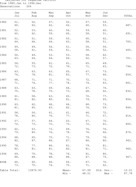
VII. APÊNDICE: INDÚSTRIA DE TRANSFORMAÇÃO (O

RELATÓRIO DO X-12-ARIMA)

Nos capítulos anteriores constam excertos das saídas do computador relativas aos

casos analisados. Na verdade, conforme já comentamos, as informações para análise

propiciadas pelo programa são muito mais volumosas e abrangem um sem número

de aspectos não comentados em nossa pesquisa. Selecionamos aquilo que nos

pareceu mais relevante e que respondia às nossas indagações. Entretanto, para que

se tenha uma idéia de toda a informação disponibilizada pelo X-12-ARIMA,

agregamos uma saída (quase) completa referente à Indústria de Transformação e ao

caso em que se analisam os efeitos da composição do mês.

U.S. Department of Commerce, Bureau of the Census

X-12-ARIMA monthly seasonal adjustment Method, Release Version 0.1.2

This method modifies the X-11 variant of Census Method II by J. Shiskin A.H. Young and J.C. Musgrave of February, 1967. and the X-11-ARIMA program based on the methodological research developed by Estela Bee Dagum, Chief of the Seasonal Adjustment

and Time Series Staff of Statistics Canada, September, 1979.

Primary Programmers: Brian Monsell, Mark Otto

Series Title- Indústria de Transformação - Brasil (IBGE) - (1991=100) Series Name- ITRANSF

05/11/98 09:24:27.55

-Period covered- 1st month,1980 to 12th month,1996. -Type of run - multiplicative seasonal adjustment.

-Sigma limits for graduating extreme values are 1.5 and 2.5. -3x3 moving average used in section 1 of each iteration, 3x5 moving average in section 2 of iterations B and C,

moving average for final seasonal factors chosen by Global MSR. -Sliding spans analysis performed.

-Spectral plots generated for selected series.

(47)

EAESP/FGV/NPP - N

ÚCLEODE

P

ESQUISAS E

P

UBLICAÇÕES

47/96

Indústria de Transformação - Brasil (IBGE) - (1991=100) PAGE 1,

SERIES ITRANSF

Line # ---

1: series title=”Indústria de Transformação - Brasil (IBGE) – (1991=100”) 2: name="ITRANSF"

3: start=1980.01 4: data=

5: 94.8 92.8 102.5 95.2 104.8 106.3 111.5 110.2 113.2 115.3 106.9 97.3 6: 94.9 94.3 95.3 89.0 92.1 95.9 99.5 96.8 94.1 96.4 90.3 82.3 7: 79.9 79.3 94.3 88.5 94.0 99.0 102.4 104.9 101.6 99.0 92.7 83.2 8: 77.4 74.8 88.5 80.0 88.7 89.5 90.3 97.9 94.1 96.2 92.4 83.7 9: 79.6 83.2 85.5 82.3 94.0 97.1 100.8 103.7 98.1 106.5 98.9 88.8 10: 91.8 85.1 94.9 84.8 96.1 99.5 110.4 112.6 110.8 121.1 109.2 99.7 11: 101.9 96.1 98.0 102.4 106.8 113.5 123.2 122.1 128.8 134.5 118.9 106.9 12: 108.7 108.7 112.7 111.7 112.9 115.7 115.1 116.1 121.7 124.5 115.8 102.6 13: 98.6 98.5 112.4 102.3 106.3 117.8 117.5 125.0 120.1 114.3 107.6 99.2 14: 96.5 88.7 102.1 100.0 112.1 123.0 126.3 134.3 125.2 128.9 118.6 101.8 15: 101.3 96.2 97.9 70.6 99.4 101.9 115.4 122.7 115.2 118.9 106.4 83.2 16: 84.6 77.7 86.1 99.0 104.9 106.2 117.5 118.6 109.2 114.3 100.5 81.5 17: 82.6 88.2 92.0 90.8 94.4 100.0 104.8 102.6 102.3 104.2 100.8 88.4 18: 86.8 87.4 105.0 99.1 107.3 108.3 113.3 113.7 109.4 109.5 108.1 96.2 19: 94.8 90.2 109.9 99.5 112.4 112.4 114.9 125.6 122.8 122.2 122.3 114.3 20: 111.4 106.6 125.0 111.6 114.2 116.3 114.7 118.2 113.3 117.8 115.4 99.9 21: 100.3 98.6 109.2 108.4 117.5 111.3 126.6 126.0 122.9 128.2 122.2 106.8 22: 107.0 101.8 113.1 116.9 120.1 122.5 127.8 128.1 131.0 135.8 120.3 102.3 23: )

24: span=(1980.1,1996.12 25: }

26:

27: transform {function=log} 28:

29: regression{ variables = (const) 30: user = (SG TR QA QI SX SB) 31: start = 1980.01

32: file = "DUSGSBDU.prn" 33: format = "(1F3.0,5f4.0)" 34: usertype = td

35: save = (rmx) 36: }

37:

38: # identify {diff=(0,1) sdiff=(0,1)} 39:

40:arima{

41:model =([5] 1 0)(2 0 0) 42: }

43: check{ 44: print=(all) 45: }

46: outlier{types=all} 47:

48: x11{} 49:

50: slidingspans { outlier = keep } 51:

(48)

EAESP/FGV/NPP - N

ÚCLEODE

P

ESQUISAS E

P

UBLICAÇÕES

48/96

RE L A T Ó R I O D E PE S Q U I S A Nº 1 6 / 1 9 9 8 Indústria de Transformação - Brasil (IBGE) - (1991=100) PAGE 2

A 1 Time series data (for the span analyzed) From 1980.Jan to 1996.Dec

Observations 204

--- Jan Feb Mar Apr May Jun

Jul Aug Sep Oct Nov Dec TOTAL --- 1980 95. 93. 103. 95. 105. 106.

112. 110. 113. 115. 107. 97. 1251. 1981 95. 94. 95. 89. 92. 96.

100. 97. 94. 96. 90. 82. 1121. 1982 80. 79. 94. 89. 94. 99.

102. 105. 102. 99. 93. 83. 1119. 1983 77. 75. 89. 80. 89. 90.

90. 98. 94. 96. 92. 84. 1054. 1984 80. 83. 86. 82. 94. 97.

101. 104. 98. 107. 99. 89. 1119. 1985 92. 85. 95. 85. 96. 100.

110. 113. 111. 121. 109. 100. 1216. 1986 102. 96. 98. 102. 107. 114.

123. 122. 129. 135. 119. 107. 1353. 1987 109. 109. 113. 112. 113. 116.

115. 116. 122. 125. 116. 103. 1366. 1988 99. 99. 112. 102. 106. 118.

118. 125. 120. 114. 108. 99. 1320. 1989 97. 89. 102. 100. 112. 123.

126. 134. 125. 129. 119. 102. 1358. 1990 101. 96. 98. 71. 99. 102.

115. 123. 115. 119. 106. 83. 1229. 1991 85. 78. 86. 99. 105. 106.

118. 119. 109. 114. 101. 82. 1200. 1992 83. 88. 92. 91. 94. 100.

105. 103. 102. 104. 101. 88. 1151. 1993 87. 87. 105. 99. 107. 108.

113. 114. 109. 110. 108. 96. 1244. 1994 95. 90. 110. 100. 112. 112.

115. 126. 123. 122. 122. 114. 1341. 1995 111. 107. 125. 112. 114. 116.

115. 118. 113. 118. 115. 100. 1364. 1996 100. 99. 109. 108. 118. 111.

127. 126. 123. 128. 122. 107. 1378. AVGE 93. 91. 101. 95. 103. 107.

112. 115. 112. 115. 107. 95. Table Total- 21183.00 Mean- 103.84 Std. Dev.- 13.05

(49)

EAESP/FGV/NPP - N

ÚCLEODE

P

ESQUISAS E

P

UBLICAÇÕES

49/96

MODEL DEFINITION Transformation Log(y)

Regression Model

Constant + User-defined ARIMA Model

([5] 1 0)(2 0 0) regARIMA Model Span

From 1980.Jan to 1996.Dec

MODEL ESTIMATION/EVALUATION

Exact ARMA likelihood estimation

Max total ARMA iterations 200 Max ARMA iter's w/in an IGLS iterati 40 Convergence tolerance 1.00E-05 OUTLIER DETECTION

From 1980.Jan to 1996.Nov Observations 203

Types AO, LS and TC Method add one

Critical |t| for AO outliers 3.8 Critical |t| for LS outliers 3.8 Critical |t| for TC outliers 3.8

The following time series values might later be identified as outliers when data are added or revised. They were not identified as outliers in this run either because their test t-statistics were slightly below the critical value or because they were eliminated during the backward deletion step of the identification procedure, when a non-robust t-statistic is used.

---

Outlier t(AO) t(LS) t(TC) ---

AO1987.Feb 3.26 2.20 3.19

LS1987.Jun -0.72 -3.29 -2.67 AO1988.Mar 3.33 2.00 2.78 LS1988.Dec 2.59 3.32 3.17 AO1995.May -3.58 -3.36 ---

Average percentage standard error in within-sample forecasts: Last year: 6.76 Last-1 year: 14.23 Last-2 year: 3.99 Last three years: 8.32

(50)

EAESP/FGV/NPP - N

ÚCLEODE

P

ESQUISAS E

P

UBLICAÇÕES

50/96

Regression Model

---

Parameter Standard

Variable Estimate Error t-value

---

Constant 0.0016 0.01143 0.14

User-defined

SG 0.0139 0.00484 2.88

TR 0.0195 0.00433 4.51

QA 0.0096 0.00404 2.38

QI 0.0255 0.00389 6.55

SX 0.0120 0.00408 2.94

SB 0.0005 0.00500 0.10

LS1981.Mar -0.1369 0.02675 -5.12

AO1984.Feb 0.0848 0.01887 4.49

TC1985.Apr -0.1356 0.02469 -5.49

LS1990.Mar -0.1088 0.02633 -4.13

AO1990.Apr -0.2701 0.01987 -13.59

TC1991.Apr 0.1255 0.02585 4.86

AO1992.Feb 0.1103 0.01930 5.72

--- Chi-squared Tests for Groups of Regressors

---

Regression Effect df Chi-Square P-Value

---

User-defined 6 153.54 0.00

--- ARIMA Model: ([5] 1 0)(2 0 0)

Nonseasonal differences: 1

Standard

Parameter Estimate Errors

--- Nonseasonal AR

Lag 5 -0.1784 0.06665

Seasonal AR

Lag 12 0.6528 0.06817

Lag 24 0.2331 0.06953

--- Likelihood Statistics

---

Effective number of observations (nefobs) 203

Number of parameters estimated (np) 18

Log likelihood 401.5066

Transformation Adjustment -940.9400

Adjusted Log likelihood (L) -539.4334

AIC 1114.8668

F-corrected-AIC 1118.5842

Hannan Quinn 1138.9938

BIC 1174.5045