Estimating economic interactions of financial suppliers in Thailand

(1)

Estimating Economic Interactions of Financial

Suppliers in Thailand

∗

Juliano J. Assunção

†

Department of Economics

Pontiﬁcal Catholic University of Rio de Janeiro, Brazil

Abstract

This paper presents a methodology to estimate and identify different kinds of eco-nomic interaction, whenever these interactions can be established in the form of spa-tial dependence. First, we apply the semi-parametric approach of Chen and Conley (2001) to the estimation of reaction functions. Then, the methodology is applied to the analysis financial providers in Thailand. Based on a sample of financial insti-tutions, we provide an economic framework to test if the actual spatial pattern is compatible with strategic competition (local interactions) or social planning (global interactions). Our estimates suggest that the provision of commercial banks and suppliers credit access is determined by spatial competition, while the Thai Bank of Agriculture and Agricultural Cooperatives is distributed as in a social planner problem.

JEL Classiﬁcation: C14, O16, O18, R12.

Key words: spatial econometrics, semi-parametric estimation,ﬁnancial suppliers.

∗ _{VERY PRELIMINAR. Please do not quote without permission.}

† _{Address: Rua Marquês de São Vicente, 225/F210, Rio de Janeiro, Brazil,}

(2)

1 Introduction

Although the interaction among agents is at the core of a large portion of the economic toolbox, it has been neglected by the traditional models in econo-metrics. The usual assumption of independence in cross-section analysis es-tablishes that the outcome of an agent is not aﬀected by the outcome of the others. Nevertheless, economic decisions might be characterized by a signiﬁ -cant degree of interdependence due to strategic behavior, sequential decisions, resource constraints, transportation costs, and others.

The purpose of this paper is twofold. First, we provide a regression model for cross-section data to estimate reaction functions which is able to contrast different types of interaction, whenever these interactions can be established in the form of spatial dependence, i.e., when the interdependence between agents can be represented as a function of some notion of distance. This approach is particularly useful because it leads to the spatial autoregressive specifications for reaction functions which are well known in the geostatistics and regional sciences [Ord (1975), Anselin (1988)]. However, the traditional parametric approach of the problem has important drawbacks because it is based on the adoption of specific functional forms of interactions.

For this task, the paper contributes using a simple adaptation of the semi-parametric approach of Chen and Conley (2001) to the generalization of the autoregressive component of these models. The semiparametric formulation allows moreﬂexible speciﬁcations. Although there is a (potential) loss of

effi-ciency if compared with the proper parametric alternatives, there is an evident gain in consistency. Since the identification of adequate parametric forms is a very hard task in empirical applications, the latter effect is more likely to prevail. It assures improvements in the estimation of substantive economic effects mentioned above and, even if spatial dependence or economic interac-tions are not an end in itself, a better estimation of the spatial autoregressive term might enhance other parameter’s estimates. In some cases, measurement errors generate artificial spatial dependence, which determines that OLS esti-mates are inconsistent.

(3)

The paper is organized as follows. Next section presents the spatial autore-gressive model in its general form. In Section 3, the semiparametric approach of Chen and Conley (2001) is used to inference. Some parametric alternatives are also discussed for the sake of completeness. The empirical application is the object of Section 4. In this section, we provide an economic framework to guide the empirical strategy and the estimates of the model. Data from the Thai Community Development Department (CDD) surveys across more than three thousand villages in four provinces of Thailand is used to characterize the proﬁle of ﬁnancial providers. Last section concludes.

2 An econometric model of interaction

Consider a set of N economic agents indexed by i. For each agent i, there is a dataset represented by (yi,x_i₎ _∈ _{< × <}K_{, where} _yi _{is a choice variable} andx_i _{is a vector of characteristics. A general linear formulation for economic} interaction can be stated as:

yi = X

i6=j

wijyj+x0iβ+ui, (1)

where the choice of agent iis determined not only for her own characteristics but also by the choice of others. Notice that in eq. (1) each agent is allowed to be affected differently by the others. Unfortunately, there is no degree of freedom for the estimation of such a general specification.

In order to estimate a model of economic interaction such as eq. (1) it is necessary to restrict the analysis to structured weights. The proposal of this paper is to use a structure induced by the notion of spatial dependence.

LetDi,j an exogenously deﬁned distance function between agents iandj. For example, it can be considered simply as Di,j = ks_i₋s_j_k_{, where} s_i _∈ _<L _is the location of agent i. Therefore, eq. (1) can be written as a general spatial autoregressive model given by:

yi = X

i6=j

g(Di,j)yj+x0iβ+ui, (2)

where ui is i.i.d. and normally distributed with mean 0 and variance σ2. The function g(·) incorporates the spatial dependence into analysis and corre-sponds to the structure needed for identiﬁcation.1

This representation

im-1 _If_D

i,j = min{i−j,0}, eq. (2) becomes the well known ARmodel in time series. In this case, sinceDi,j = 0for all i < j, eq. (2) can be written as

(4)

plies that the value ofyj, for everyj 6=i, aﬀectsyi through the spatial weight g(Di,j). If g(·) is equal to zero there is no interaction and eq. (2) can be es-timated by OLS, which provides an eﬃcient and consistent estimate for β. If g(·)6= 0, there is spatial dependence and economic interaction is relevant for the estimation of β.

Using matrix notation, eq. (2) can be expressed as:

Y₌AY₊X_β₊u_, ₍₃₎

where A₌          

0 g(D1,2) · · · g(D1_,N)

g(D2,1) 0 · · · g(D2,N) ... ... . .. ... g(DN,1) g(DN,2) · · · 0

          . (4)

In this case,Y_{is normally distributed with mean}₍I₋A₎−1X_β_{and covariance} matrix C_≡_σ2

(I₋A₎−1₍I₋A₎−1_.

The properties of estimators and hypothesis tests for eq. (2) are derived from the asymptotics for stochastic processes. As in time series analysis, regularity conditions are needed to limit the extent of spatial dependence in order to assure consistency and asymptotic normality. In fact, eq. (2) deﬁnes a station-ary stochastic process with higher-order moments ifρ(A₎_<₁_{, where} _ρ₍A₎_is the spectral radius of A_.2

3 Estimation

The log-likelihood of eq. (2) can be expressed as:

lnL=−N

2 log 2π−

N

2 logσ

2

− 1

2σ2 N X

i=1



yi−X

i6=_j

g(Di,j)yj−x0 iβ

 

2

. (5)

Although we consider two diﬀerent approaches to estimate eq. (2), we focus on the semiparametric estimation of eq. (2) since the parametric approach is treated in a large body of literature [e.g. Anselin (1988, 2001)].

Therefore, an AR(1) model can be represented by the function g(D) =

  

α, ifD= 1 0, otherwise

.

2

(5)

3.1 Parametric Estimation

Ord (1975) presents a parametric approach to eq. (2) in which the function g(·) is assumed to be known up to a constant. Formally,g(·) takes the form of

g(Di,j) =ρw(Di,j), (6) wherew(·)is a (known) function deﬁning the matrix of spatial weights. Using matrix notation and deﬁning W _≡[w(Di,j)], eq. (3) becomes

Y₌_ρWY₊X_β₊u_. ₍₇₎

This model can be properly estimated by maximum likelihood.3

The condition required for stationarity in this case can be simpliﬁed to 1

λ <|ρ| < 1 ¯

λ, where λ andλ¯ are the minimum and maximum eigenvalue of W_{, respectively.}

3.2 Semiparametric Estimation

Chen and Conley (2001) suggest a semiparametric approach to spatial models for univariate panel data. Herein, an adaptation of this approach is applied to the model (3), allowing for a general form of g(·). An estimator forg(·) is constructed by the method of sieves. This method uses aﬂexible sequence of parametric families to approximateg(·).

As Chen and Conley (2001), a shape-preserving cardinal B-spline sieve is used to facilitate the test of shape restrictions. LetBm denote the cardinal B-spline of order m, deﬁned as:

Bm(x) = 1 (m₋1)!

m X

k=0

(₋1)k

µ_m

k ¶

[max (0, x₋k)]m−1.

Notice that Bm is m ₋1 times diﬀerentiable, nonnegative and symmetric

around the center of its support [0, m]. Therefore, the function g(·) can be approximated by

g(D)_≈

¯ K X

k=K

akBm(2nD−k), (8)

whereK¯ andKdetermine the accuracy of the approximation andnis an index which provides a scale reﬁnement.4

This approximation allows the formulation

3

See Anselin (1988, 2001) for comprehensive expositions of the model (7). 4

(6)

of useful restrictions in the shape of g(·). For example,g(·) is non-increasing if ak _≥ak+1 for allk.

Substituting eq. (8) into eq. (5) and rearranging we obtain the following like-lihood:

lnLsp =₋N

2 log 2π−

N

2 logσ

2

− 1

2σ2 N X

i=1

(yi₋z0

iα−x0iβ) 2

, (9)

where z_i _{= (}P_i₆₌_j_Bm₍₂n_Di,j ₋_K₎_{yj, ...,} P_i₆₌_j_Bm³₂n_Di,j ₋_K¯´_yj₎ _and _α ₌ ³

aK, .., a_K¯ ´

. As a consequence, the MLE of the vector (α, β) coincides with the OLS estimator of a regression ofyi onz_i _andx_{i. And} _σ2

can be estimated by σˆ2

= 1 N

PN

i=1(yi−z0_iα−x0_iβ) 2

. Although this formulation is more ﬂexible about the shape of the g(·) function, the computation of the sieve estimator is relatively simple.

4 Application: Financial suppliers in Thailand

This section applies the methodology above to study the profile of financial suppliers in Thailand. One important branch of the economic development literature focus on financial deepening. As suggested by Greenwood and Jo-vanovic (1990), the access to (costly)financial instruments enhances risk shar-ing and generates economic growth. The economy-wide wealth accumulation process, in turn, affects the access tofinancial intermediaries. This model gen-erates a dynamic relationship between the wealth distribution and the par-ticipation in the financial sector. Therefore, the analysis of the provision of

ﬁnancial services arises as a key element of the development process.

Diﬀerent from recent empirical studies, more interested to evaluate the role of theﬁnancial deepening channel,5

this section investigates the type of eco-nomic interaction amongﬁnancial providers prevail in our sample. We contrast two kinds of interactions; namely, strategic spatial competition and central planning. Our empirical strategy is based on the comparison of reaction func-tions derived from the those diﬀerent economic environments.

4.1 Economic background

Let us start with the case of strategic spatial competition, in which those reaction functions are determined locally. Since the 1929 inﬂuential paper

5

(7)

by Hotelling, interesting features of the problem motivated many economists to study the location of ﬁrms in many situations - introducing or not price diﬀerentiation, analyzing simultaneous versus sequential decisions, varying the shape of the markets, the existence of relocation costs, and so on.6

Behind most of these models, it is possible to obtain reaction functions that ex-hibit local dependence in a relatively general setup. Consider a one-dimensional county where consumers are distributed along the interval [0,1] according to the distribution function F(·). Each consumer x_∈ [0,1] contracts one fi nan-cial operation from the cheapest source. Suppose that in a cross-section survey we observe the provision ofN bank agencies providing identical services offi -nancial intermediation in different locations bi, for i = 1, ..., N. Without loss of generality, we label those observations in a way such thatb1 < b2 < ... < bN. Next, we will derive general reaction functions for different assumptions about the interaction of these agencies in order to identify a test about the decision process behind the observed pattern.

Letx∗

i be the consumer who is indiﬀerent between banks iandi+ 1, which is deﬁned by the condition

pi+t(x∗_i −bi) =pi+1+t(bi+1−x∗_i),

where pi is the price charged by bank i, t is the (linear) transportation cost, b0 = 0 andbN+1 = 1. Equivalently, it is easy to check that

x∗_i = pi+1−pi 2t +

bi+1+bi

2 .

Therefore, the market size of bank i is given by F (x∗_i) −F ³x∗_i₋1 ´

, which depends only on the provision of nearby services of banks i₋1 and i+ 1.7 Consequently, the decision of setup a bank in a location bi is not aﬀected by the location of banks which are not neighbors. And more important, this result does not depend on the type of strategic interaction we are dealing with. It can be simultaneous (as a Cournot oligopoly) or sequential (as a Stackelberg leadership). What really matters is the strategic behavior - banks presumably decide individually based on available information and expectations about the behavior of the opponents. As a result, the reaction function of bankiin such situations is expressed in terms of prices and locations of adjacent banksi−1

andi+ 1.

6

See Hotelling (1929), Eaton and Lipsey (1975) and Prescott and Visscher (1977). For the existence of equilibrium of such games in situations with discontinuous payoﬀs, see Dasgupta and Maskin (1986).

7 _{Notice that the individual} _x_∗

i lives in the center of banksiand i+ 1 ifpi+1 =pi. In addition, if consumers are uniformly distributed, the market size simpliﬁes to

(8)

In summary, the strategic behavior of banks leads to local spatial interaction. Notwithstanding whether decisions are made sequentially or not, theﬁnancial provision in a given region is determined by the adjacent neighborhood.

On the other hand, if the provision of the services is deﬁned by a social planner, in a resource allocation problem, the interaction is global. To be more precise, let W(b1, ..., bN) denote the social welfare associated with the existence of banks at locationsb1, ..., bN. If the setup cost of each banki isci, the problem of a social planner with a budgetI is given by:

max

b1,...,bN

W(b1, ..., bN)

subject to

N X

i=1

cibi =I.

It is straightforward to check that the ﬁrst-order conditions of this problem implies that

bi = λ

∂W/∂bi



I₋X j6=i

cjbj

 ,

where λ is the multiplier related to the budget constraint. Note that, in the social planner problem, the position of bank i is aﬀected by all other banks, even if W is separable, because of the budget constraint. Therefore, we ex-pect to observe global interactions in public provision of bank services and local interactions whenever the locations are deﬁned privately by strategic competition.

4.2 Data

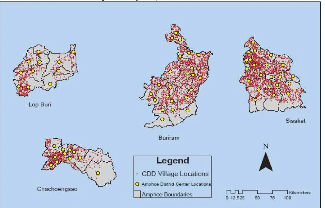
We consider data from four of Thailand’s 73 provinces (changwats) - the semi-urban provinces of Chachoengsao and Lop Buri in the Central region relatively near Bangkok, and the more rural Sisaket and Buriram in the poorer Northeast region (seeﬁgure 1). Each village was vectorized into a Geographic Information System.

(9)

provinces selected can be ordered in economic terms decreasing from Chacho-engsao to Lop Buri to Buriram to Sisaket.

The data used hereafter is extracted from the Thai Community Development Department (CDD) survey, conducted every two year from 1986-1996. Figure 2 shows a total of 3391 geo-located villages which were linked to the CDD database. There are 1300 villages in Sisaket, 1230 in Buriram, 419 in Lop Buri and 442 in Chachoengsao. Despite the availability of a panel, the following analysis considers only data from 1996.

Thailand is a very interesting case study for us. During the period from 1976 to 1996, the real GNP per capita grew at 5.7% annually whileﬁnancial partic-ipation increased from 6% in 1976 to 26% in 1996. The fraction of population that did not participate in ﬁnancial intermediation and was not engaged in entrepreneurial activities fell from 80% to 60%.

From the CDD database, there are binary variables indicating the presence or absence of credit providers. The Thai Bank of Agriculture and Agricultural Cooperatives (BAAC) had the highest number of villages reporting its access, ranging from 85% in Chachoengsao to 69% in Sisaket. It is also used variables reporting the suppliers credit access (62% in Chachoengsao) and commercial banks (34% in Chachoengsao).

A wealth index was created using a principal component analysis of four vari-ables - per capita TVs per village, per capita motorcycles per village, per capita pick-up trucks per village, and the percentage of household havingﬂush toilets per villages. The other variables used from the CDD database are the percent-age of individuals per villpercent-age having completed secondary education and two measures of soil quality.

In addition to variables gathered from the CDD database, a measure of prox-imity to major roads is constructed to represent transportation or distances costs. For each village, the shortest route along road networks in terms of travel time to the nearest major highway was mapped, and the travel time calculated. Figure 3 shows the road networks and major intersection locations in each changwat.

4.3 Empirical Results

In this section, we use the econometric model presented in Section 2 to iden-tify what type of economic interaction has generated the observed pattern of

(10)

im-poses a strong relationship among all the bank agencies provided by a social planner, we should observe only local interactions for the case of strategic competition.

The degree of interaction in the econometric analysis is captured by the func-tiong(·), which can is estimated below. As long as our sample includes villages which are not homogeneous with respect to observable variables, we also in-troduce some control variables to account for those diﬀerences.

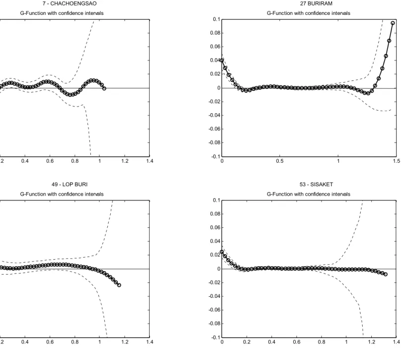
The results are presented in Tables 1 to 3, while the estimated g functions are depicted in Figures 4 to 6. All estimations are based in the following speciﬁcation:

provider_i =X

j6=_i

g(Di,j)provider_j+β0+β1wealthi+β2ADVi (10)

+β3Dis2Maj_i+β4Soil1i+β5Soil5i+ui,

where provider is the binary variable indicating the presence or not of the corresponding ﬁnancial intermediary, wealth is the wealth index, ADV is the percentage of individuals per village having completed secondary education,

Dis2Majis the length of the shortest route to the nearest major highway,Soil1

and Soil5 are two measures of soil quality. Equation (10) was estimated for each provider and each province.

Figure 4 present the estimated g function for the Thai Bank of Agriculture and Agricultural Cooperatives (BAAC). As we could expect, the spatial dis-tribution of BAAC is compatible with the central planner solution. There is no signiﬁcant reduction in the relationship among villages as we increase the distance between them. This patterns is present in all four provinces consid-ered. On the other hand, Figures 5 and 6 suggest that the process behind the provision of commercial banks and suppliers credit access due to strate-gic competition. Except for the province of Lop Buri, where theg function is not signiﬁcant, there is a clear pattern of local interaction in Chachoengsao, Buriram and Sisaket.

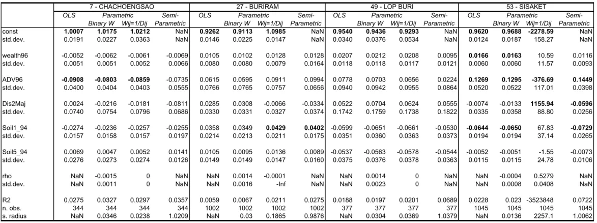
In addition to analyze the provision of financial services in Thailand, we are also interested in the comparison of the results obtained from different specifi -cations. Based on this, Tables 1 to 3 present 4 columns for each province. The

ﬁrst one corresponds to the OLS estimation of (10), assuming that g(D) = 0

for allD_≥0. Second and third columns present two diﬀerent parametric spec-iﬁcations commonly used in the spatial econometrics literature.8

The speciﬁ

-8

(11)

cation with a binaryW matrix implies that

g(D) =

    

ρ, if D_≤c;

0, otherwise;

while the speciﬁcation with the inverse of distance matrix (column 3) is g(D) = _Dρ for all D. Finally, the last column shows the estimates of the parameters considering the semiparametric formulation for the spatial autore-gressive term.

From the comparison of the results depicted in Tables 1 to 3, we learn that the OLS or parametric estimates ofg can mislead the estimation of the other pa-rameters of the regression. Specially for the case of the BAAC in Sisaket, where the semi-parametric estimate of g is very precise and very distinct from the functional forms traditionally used in spatial econometrics, we get significant differences. The coefficient of wealth is not significant in the semi-parametric specification and significant in the others. For the case of distance to major roads, we observe the opposite.

5 Conclusion

This paper provides an econometric analysis of economic interactions for sit-uations that can be represented by spatial dependence. We provide both an econometric model and an economic framework that can be combined to iden-tify important features of the interaction among economic agents. In particu-lar, we have applied the methodology to study the proﬁle ofﬁnancial suppliers in Thailand.

The econometric model presented here is a straightforward adaptation of the semi-parametric approach to spatial problems developed by Chen and Conley (2001). This simple adaptation enable us to estimate reaction functions which are at the core of the empirical strategy adopted to investigate economic inter-actions. Theﬂexibility to estimate the functional form of the spatial structure is a clear advance with respect to the traditional parametric approach sug-gested by Ord (1975), whose recent developments can be found in Anselin (2001). A better accounting of spatial dependence is not only a more accurate measure of the interaction between agents but also a means of improving the estimation of the other parameters of the regression.

(12)

what kind of reaction functions is more likely to produce these observations as an equilibrium. We show that a general model of strategic can be associ-ated to local reaction functions, i.e., the location of a given bank is aﬀected only by their neighborhood. On the other hand, in a typical social planner problem, the budget constraint imposes a global structure of interdependence among the locations of the banks. Our estimates suggest that the Thai Bank of Agriculture and Agricultural Cooperatives is more likely to be spatially dis-tributed according to a social planner problem (global interaction), while the provision of commercial banks and suppliers credit access is deﬁned by spatial competition (local interaction).

References

[1] Anselin, L. (1988). Spatial Econometrics: Methods and Models, Kluwer Academic Publishers, Dordrecht, The Netherlands.

[2] Anselin, L. (2001). “Spatial econometrics”. In Baltagi, B., ed., A Companion to Theoretical Econometrics, pages 310—330. Blackwell, Oxford.

[3] Anselin, L. (2002) “Under the Hood: Issues in the Speciﬁcation and Interpretation of Spatial Regression Models”, Agricultural Economics 17(3): 247-267.

[4] Chen, X. and T. G. Conley (2001) “A new semiparametric spatial model for panel time series”,Journal of Econometrics, 105: 59-83.

[5] Dasgupta, P. and E. Maskin (1986) “The existence of equilibrium in discontinuous economic games, II: application”, Review of Economic Studies, 53(1): 27-41.

[6] Eaton, B. C. and R. G. Lipsey (1975) “The principle of minimum diﬀerentiation reconsidered: some new developments in the theory of spatial competition”,

Review of Economic Studies,42(1): 27-49.

[7] Felkner, J. S. and R. M. Townsend (2003) “The Wealth of Villages: an application of GIS and spatial statistics to economic models”, National Opinion Research Center, University of Chicago, mimeo.

[8] Hotelling, H. (1929) “Stability in competition”, Economic Journal, 39(153): 41-57.

[9] Ord, K. (1975) “Estimation methods for models of spatial interaction”,Journal of the American Statistical Association, 70(349): 120-126.

[10] Jeong, H. and R. M Townsend (2003) “Models of growth and inequality: an evaluation”, National Opinion Research Center, University of Chicago, mimeo.

(13)

(14)

(15)

(16)

Figure 4 - Semiparametric Estimates of G - BAAC

49 - LOP BURI 53 - SISAKET

7 - CHACHOENGSAO 27 BURIRAM

0 0.2 0.4 0.6 0.8 1 1.2 1.4

-0.01 -0.008 -0.006 -0.004 -0.002 0 0.002 0.004 0.006 0.008 0.01

G-Function with confidence intervals

0 0.5 1 1.5

-0.01 -0.008 -0.006 -0.004 -0.002 0 0.002 0.004 0.006 0.008 0.01

-0.006 -0.004 -0.002 0 0.002 0.004 0.006 0.008 0.01

(17)

Figure 5 - Semiparametric Estimates of G - Commercial Banks

0 0.1 0.2 0.3 0.4 0.5 0.6 0.7 0.8 0.9 1 -0.05

-0.04 -0.03 -0.02 -0.01 0 0.01 0.02 0.03 0.04 0.05

0 0.5 1 1.5

-0.05 -0.04 -0.03 -0.02 -0.01 0 0.01 0.02 0.03 0.04

-0.03 -0.02 -0.01 0 0.01 0.02 0.03 0.04 0.05

-0.03 -0.02 -0.01 0 0.01 0.02 0.03 0.04

(18)

Figure 6 - Semiparametric Estimates of G - Suppliers Credit Access

0 0.2 0.4 0.6 0.8 1 1.2 1.4

-0.1 -0.08 -0.06 -0.04 -0.02 0 0.02 0.04 0.06 0.08 0.1

0 0.5 1 1.5

-0.1 -0.08 -0.06 -0.04 -0.02 0 0.02 0.04 0.06 0.08 0.1

-0.06 -0.04 -0.02 0 0.02 0.04 0.06 0.08 0.1

(19)

OLS Semi- OLS Semi- OLS Semi- OLS Semi-Binary W Wij=1/Dij Parametric Binary W Wij=1/Dij Parametric Binary W Wij=1/Dij Parametric Binary W Wij=1/Dij Parametric const 1.0007 1.0175 1.0212 NaN 0.9262 0.9113 1.0985 NaN 0.9540 0.9436 0.9293 NaN 0.9620 0.9688 -2278.59 NaN std.dev. 0.0191 0.0227 0.0363 NaN 0.0146 0.0225 0.0147 NaN 0.0340 0.0376 0.0534 NaN 0.0124 0.0187 158.27 NaN

wealth96 -0.0052 -0.0062 -0.0061 -0.0069 0.0105 0.0102 0.0128 0.0128 0.0207 0.0212 0.0208 0.0095 0.0166 0.0163 _10.59 _0.0116 std.dev. 0.0051 0.0051 0.0052 0.0066 0.0080 0.0080 0.0079 0.0164 0.0118 0.0118 0.0117 0.0121 0.0060 0.0060 11.57 0.0093

ADV96 -0.0908 -0.0803 -0.0859 _-0.0735 _0.0615 _0.0595 _0.0911 _0.0994 _0.0778 _0.0703 _0.0656 _0.0224 0.1269 0.1295 -376.69 0.1449 std.dev. 0.0400 0.0404 0.0403 0.0555 0.0766 0.0765 0.0757 0.0656 0.0940 0.0942 0.0955 0.0864 0.0520 0.0522 117.01 0.0398

Dis2Maj 0.0024 -0.0216 -0.0181 -0.0811 0.0285 0.0308 -0.0066 -0.0334 0.0522 0.0704 0.0624 0.0555 -0.0074 -0.0133 1155.94 -0.0596 std.dev. 0.0740 0.0754 0.0796 0.0686 0.0330 0.0331 0.0327 0.0374 0.1742 0.1759 0.1738 0.1822 0.0335 0.0358 88.80 0.0256

Soil1_94 -0.0274 -0.0236 -0.0257 -0.0255 0.0358 0.0349 0.0429 0.0402 -0.0599 -0.0651 -0.0661 -0.0530 -0.0644 -0.0650 67.83 -0.0729 std.dev. 0.0157 0.0158 0.0157 0.0197 0.0214 0.0213 0.0211 0.0175 0.0351 0.0360 0.0363 0.0373 0.0194 0.0194 37.14 0.0265

Soil5_94 0.0069 0.0047 0.0052 0.0141 0.0105 0.0095 0.0136 0.0089 -0.0537 -0.0563 -0.0578 -0.0544 -0.0052 -0.0051 -1.55 -0.0073 std.dev. 0.0276 0.0273 0.0274 0.0126 0.0149 0.0149 0.0147 0.0160 0.0375 0.0376 0.0378 0.0363 0.0115 0.0115 24.78 0.0106

rho NaN -0.0015 0 NaN NaN 0.0014 -0.0001 NaN NaN 0.0014 0 NaN NaN -0.0004 0.5279 NaN

std.dev. NaN 0.0011 0 NaN NaN 0.0016 -Inf NaN NaN 0.0023 0 NaN NaN 0.0008 0.0408 NaN

R2 0.0275 0.0327 0.0297 0.0357 0.0059 0.0067 0.0211 0.0275 0.0188 0.0197 0.0201 0.0689 0.0228 0.023 -3523848 0.0722

n. obs. 344 344 344 344 1002 1002 1002 1002 377 377 377 377 1045 1045 1045 1045

s. radius NaN 0.0346 0.0238 1.0209 NaN 0.03 0.1865 0.9876 NaN 0.0304 0.0369 1.0379 NaN 0.0136 2257.1 1.0062

7 - CHACHOENGSAO 27 - BURIRAM 49 - LOP BURI 53 - SISAKET

Table 1 - _{Results for the Thai Bank of Agriculture and Agricultural Cooperatives (BAAC)}

(20)

OLS Semi- OLS Semi- OLS Semi- OLS Semi-Binary W Wij=1/Dij Parametric Binary W Wij=1/Dij Parametric Binary W Wij=1/Dij Parametric Binary W Wij=1/Dij Parametric const 0.6633 0.5383 0.2871 NaN 0.3644 0.2399 0.1081 NaN 0.3524 0.2915 0.2542 NaN 0.2754 0.0831 -0.49 NaN std.dev. 0.0652 0.0702 0.0945 NaN 0.0324 0.0345 Inf NaN 0.0614 0.0633 0.0837 NaN 0.0335 0.0326 -Inf NaN

wealth96 -0.0588 -0.0472 -0.0381 -0.0452 -0.0422 -0.0427 -0.0466 _-0.0388 _-0.0291 _-0.0271 _-0.0290 _-0.0248 _-0.0155 _-0.0094 _-0.02 _-0.0175 std.dev. 0.0174 0.0170 0.0172 0.0182 0.0178 0.0171 0.0176 0.0220 0.0213 0.0210 0.0211 0.0223 0.0161 0.0149 0.02 0.0162

ADV96 -0.0807 -0.1425 -0.1326 -0.0890 0.2415 0.1983 0.1779 0.1697 0.5436 0.4633 0.4796 0.5093 0.5802 0.4382 0.46 0.4767 std.dev. 0.1366 0.1340 0.1332 0.1439 0.1698 0.1631 0.1671 0.1641 0.1694 0.1677 0.1714 0.1729 0.1399 0.1291 0.13 0.1422

Dis2Maj -1.1430 -0.8255 -0.6216 -0.6638 _0.0228 _0.0231 _0.0538 _-0.0602 _0.4411 _0.5502 _0.4757 _0.5732 _-0.0760 _0.1018 0.35 _0.0341 std.dev. 0.2526 0.2526 0.2592 0.3230 0.0730 0.0701 0.0718 0.0880 0.3140 0.3117 0.3123 0.2943 0.0898 0.0833 0.08 0.1062

Soil1_94 0.1215 0.0686 0.0792 0.0372 -0.0848 -0.0879 -0.0962 -0.1046 0.0395 -0.0092 0.0079 0.0143 0.0994 0.0875 0.09 0.0702 std.dev. 0.0536 0.0532 0.0523 0.0509 0.0476 0.0457 0.0469 0.0469 0.0633 0.0638 0.0651 0.0662 0.0520 0.0479 0.05 0.0556

Soil5_94 0.1840 0.1642 0.1798 0.1847 _-0.0211 _-0.0380 _-0.0297 _-0.0406 _0.0158 _-0.0024 _-0.0016 _0.0239 _0.0257 _0.0118 _0.02 _0.0092 std.dev. 0.0940 0.0911 0.0908 0.0847 0.0330 0.0317 0.0325 0.0346 0.0677 0.0671 0.0680 0.0618 0.0309 0.0285 0.03 0.0260

rho NaN 0.0155 0.0003 NaN NaN 0.0345 0.0002 NaN NaN 0.017 0.0001 NaN NaN 0.037 0.0005 NaN

std.dev. NaN 0.0036 0 NaN NaN 0.0041 Inf NaN NaN 0.0046 0.0001 NaN NaN 0.002 Inf NaN

R2 0.1411 0.1799 0.1884 0.2233 0.0117 0.0836 0.0323 0.079 0.0405 0.0608 0.0455 0.0607 0.0236 0.1664 0.0934 0.1253

n. obs. 343 343 343 343 995 995 995 995 375 375 375 375 1038 1038 1038 1038

7 - CHACHOENGSAO 27 - BURIRAM 49 - LOP BURI 53 - SISAKET

Parametric Parametric Parametric Table 2 - _{Results for Commercial Banks}

(21)

OLS Semi- OLS Semi- OLS Semi- OLS Semi-Binary W Wij=1/Dij Parametric Binary W Wij=1/Dij Parametric Binary W Wij=1/Dij Parametric Binary W Wij=1/Dij Parametric const 0.5459 0.3756 0.2160 _NaN 0.3951 0.2192 -0.1687 _NaN 0.6011 0.6138 0.7254 _NaN 0.4582 0.2877 _-0.20 _NaN std.dev. 0.0729 0.0725 0.0977 NaN 0.0337 0.0346 0.0075 NaN 0.0611 0.0666 0.1009 NaN 0.0342 0.0356 -Inf NaN

wealth96 0.0204 0.0289 0.0340 0.0287 0.0166 0.0117 0.0090 0.0106 0.0228 0.0231 0.0251 0.0355 0.0229 0.0117 0.01 0.0032 std.dev. 0.0194 0.0184 0.0192 0.0192 0.0186 0.0173 0.0179 0.0167 0.0212 0.0211 0.0210 0.0182 0.0166 0.0160 0.02 0.0143

ADV96 -0.0747 -0.1677 -0.1291 -0.1241 0.5115 0.3981 0.3926 0.4083 _-0.2206 _-0.2118 _-0.1783 _-0.1694 _0.2666 _0.1530 _0.17 _0.1354 std.dev. 0.1527 0.1456 0.1500 0.1405 0.1766 0.1647 0.1698 0.1524 0.1692 0.1687 0.1703 0.1714 0.1429 0.1371 0.14 0.1351

Dis2Maj 0.4455 0.5980 0.7203 _0.3788 _0.0946 _0.0746 0.1670 _-0.0718 _0.5541 _0.5443 _0.5643 _0.5927 -0.3887 -0.1784 _0.07 _-0.0072 std.dev. 0.2824 0.2677 0.2822 0.3474 0.0759 0.0707 0.0730 0.0755 0.3136 0.3143 0.3111 0.3273 0.0917 0.0894 0.09 0.1216

Soil1_94 -0.0770 -0.0760 -0.0817 -0.0814 0.0596 0.0196 0.0209 0.0058 -0.0822 -0.0766 -0.0604 -0.0546 -0.0559 -0.0370 -0.03 -0.0378 std.dev. 0.0598 0.0573 0.0585 0.0585 0.0494 0.0461 0.0475 0.0493 0.0630 0.0639 0.0647 0.0648 0.0532 0.0510 0.05 0.0556

Soil5_94 0.0348 0.0480 0.0527 0.0425 -0.0513 -0.0463 -0.0461 -0.0400 -0.0076 -0.0057 0.0076 0.0035 -0.0950 -0.0941 -0.09 -0.1047 std.dev. 0.1052 0.0993 0.1026 0.0860 0.0344 0.0320 0.0331 0.0310 0.0675 0.0676 0.0679 0.0688 0.0315 0.0302 0.03 0.0316

rho NaN 0.0296 0.0003 NaN NaN 0.0393 0.0004 NaN NaN -0.0033 -0.0001 NaN NaN 0.0274 0.0004 NaN

std.dev. NaN 0.0032 0.0001 NaN NaN 0.0033 Inf NaN NaN 0.0062 0.0001 NaN NaN 0.0022 Inf NaN

R2 0.0262 0.1191 0.0623 0.1873 0.0145 0.1405 0.0811 0.145 0.0245 0.0251 0.0309 0.0587 0.0272 0.1029 0.0845 0.086

n. obs. 344 344 344 344 990 990 990 990 376 376 376 376 1039 1039 1039 1039

27 - BURIRAM 49 - LOP BURI 53 - SISAKET

Table 3 - _{Results for Suppliers Credit Access}