Matheus Pereira Porto
Theoretical and experimental studies on boiling
heat transfer for the zeotropic mixture R-407C
Matheus Pereira Porto
Theoretical and experimental studies on boiling heat
transfer for the zeotropic mixture R-407C
Submitted in partial fulfillment of the requi-rements for the degree of Doctorate in Me-chanical Engineering in the Programa de Pós Graduação em Engenharia Mecânica da Uni-versidade Federal de Minas Gerais at Belo Horizonte, 2013.
Universidade Federal de Minas Gerais – UFMG
Escola de Engenharia da UFMG
Programa de Pós-Graduação em Engenharia Mecânica da UFMG
Advisor: Luiz Machado
Co-advisor: Carlos F. M. Coimbra
Matheus Pereira Porto
Theoretical and experimental studies on boiling heat transfer for the zeotropic mixture R-407C/ Matheus Pereira Porto. – Belo Horizonte, Brazil,
2013-83p. : il. (algumas color.) ; 30 cm. Advisor: Luiz Machado
Doctoral Thesis – Universidade Federal de Minas Gerais – UFMG Escola de Engenharia da UFMG
Matheus Pereira Porto
Theoretical and experimental studies on boiling heat
transfer for the zeotropic mixture R-407C
Submitted in partial fulfillment of the requirements for the degree of Doctorate in Mechanical Enginee-ring in the Programa de Pós Graduação em Enge-nharia Mecânica da Universidade Federal de Minas Gerais at Belo Horizonte, 2013.
Approved in Belo Horizonte, Brazil, september 13, 2013:
Luiz Machado Advisor - PPGMEC
Carlos F. M. Coimbra Co-advisor - UCSD
Ricardo Nicolau Nassar Koury Professor - PPGMEC
Antônio Augusto Torres Maia Professor - PPGMEC
Carlos Umberto da Silva Lima Professor - UFPA
Antônio Carlos Lopes da Costa Researcher - CDTN
Abstract
List of figures
Figure 1 – Schematical of the four parallel circuits experimental facility. . . 23
Figure 2 – Schematical of the experimental facility. In primary circuit, letters:
a, condenser; b, liquid bottle; c, micropump; d, electrical motor with inverter; e, butterfly valve; f, pre-heater; g, test section; numbers: 1, 4, 6 and 12, absolute pressure transmitters; 13, differential pressure transmitter; 3, Flow meter; 2, 5, 7 - 11, thermocouples. In cold water circuit, letters: h, ethylene-glycol tank; n, temperature controller; o, pump 2 hp; numbers: 14 - 16 and 25, thermocouples. In auxiliary circuit,letters: i, evaporator; j, compressor with inverter; k, condenser; m, expansion valve; numbers: 17, 20, 21, 23, thermocouples; 18, 19, pressure transmitter; 22, mass flow meter. In hot water circuit,
letters: l, water tank. . . 25
Figure 3 – Motor, coupling and magnetically driven micropump. . . 26
Figure 4 – Pre-heater and varistor. . . 26
Figure 5 – Determination of the experimental heat transfer coefficient, see Eq. 1.1; where, 𝑅1= 2Þ 𝑟11𝐿 ℎ, and 𝑅2=
𝑙𝑛𝑟2
𝑟1
2Þ 𝑘 𝐿. . . 27
Figure 6 – Refrigeration capacity for the auxiliary circuit in function of evapora-tion temperature (1), using 50◇
𝐶 of condensing temperature. . . 30
Figure 7 – Pattern flow map to the R-407C, at 15◇
𝐶, 10 𝑘𝑊/𝑚2 and 20 𝑙𝑝ℎ:
reference to the water. . . 31
Figure 8 – Measurements of temperature and pressure, showing an example of the variability presented during the steady state experiments in the test section. . . 33
Figure 9 – Pressure versus Enthalpy diagram for the R-407C. . . 37
Figure 10 – Example of a phase change inside a fluid passing through a tube eva-porator. . . 41
Figure 11 – Flow pattern map for refrigerant R-22 for saturation temperature of 8◇
C, an internal diameter of 12.97 mm, and heat flux of 5 𝑘𝑊 𝑚⊗2
. . . 43
Figure 12 – Comparison between the temperature profile in a pure refrigerant and in a mixture according (2). . . 49
Figure 13 – Example of an air evaporator with detailed and uncommon external geometry (3). . . 51
Figure 15 – Control volume and vapor and liquid distributions in a cross-section in a two-phase flow (e.g. evaporation region). . . 53
Figure 16 – Classical and modified Otaki method conceptual map. . . 58
Figure 17 – Comparison between the general relation proposed for pure and azeo-tropic fluids (see Eq. 3.1), Gungor and Winterton (4), Kandlikar (5), Watellet (6) and the experimental data set for R134a. . . 62
Figure 18 – Comparison between the general relation proposed for pure and azeo-tropic fluids (see Eq. 3.1), Gungor and Winterton (4), Kandlikar (5), Watellet (6) and the experimental data set for R404a. . . 62
Figure 19 – Comparison between the general relation proposed for pure and azeo-tropic fluids (see Eq. 3.1), Gungor and Winterton (4), Kandlikar (5), Watellet (6) and the experimental data set for R22. . . 63
Figure 20 – Top: Flow pattern map and experimental points for the fluid R-22. Bottom: comparison between different methodologies for determining the HTC for R-22. HTC3 = Proposed relation; HTC1a = Strictly empirical relation; HTC4b = Artificial neural network relation. . . 64
Figure 21 – First experimental validation of the proposed relation for pure fluids (Eq. 3.1), modified relation for mixtures (Eq. 3.2), applied to the re-frigerant fluid R-407C at 12 𝑘𝑊 𝑚⊗2
; Porto et al. (Eq. 3.1), Gungor and Winterton (4), Kandlikar (5), Watellet (6) and Modified Gungor Winterton (Eq. 3.3) were also used to correlate the experimental data. 65
Figure 22 – Second experimental validation of the proposed relation for pure fluids (Eq. 3.1), modified relation for mixtures (Eq. 3.2), applied to the re-frigerant fluid R-407C at 12𝑘𝑊 𝑚⊗2
; Porto et al. (Eq. 3.1), Gungor and Winterton (4), Kandlikar (5), Watellet (6) and Modified Gungor Winterton (Eq. 3.3) were also used to correlate the experimental data. 66
Figure 23 – Third experimental validation of the proposed relation for pure fluids (Porto et al., Eq. 3.1), modified relation for mixtures (Modified Porto et al., Eq. 3.2), applied to the refrigerant fluid R-407C at 12𝑘𝑊 𝑚⊗2
; Gungor and Winterton (4), Kandlikar (5), Watellet (6) and Modified Gungor Winterton (Eq. 3.3) were also used to correlate the experimen-tal data. . . 66
Figure 24 – Experimental results for using the methodology 1 (Otaki + Rouhani). . 67
Figure 25 – Experimental results for using the methodology 2 (Otaki + Hughmark). 68
Figure 26 – Experimental results for using the methodology 3 (modified Otaki + Rouhani). . . 68
List of tables
Table 1 – Primary circuit dimensions. . . 28
Table 2 – Experimental data sets for different operational conditions. . . 31
Table 3 – Uncertainty values for the primary and cold water circuit instruments. . 32
Table 4 – Uncertainty values for the auxiliary circuit instruments. . . 32
Table 5 – Student t-factor to determine the coverage factor for a level of confidence of 95%. . . 34
Table 6 – Glide to be observed for the pressure range used during the experiments. 38
Table 7 – Heat transfer coefficient relations used in this work. . . 44
Table A.1 –Input parameters considered in the search for HTC correlations . . . 46
Table A.2 –Factor K of Hughmark correlation as a function of the Z-parameter (7). 55
Table A.3 –Error metrics for the different general HTC relations, considering mean absolute percentage error (MAPE) and root mean square percentage error (RMSPE). . . 63
List of abbreviations and acronyms
HTC Heat transfer coefficients
R Refrigerant
PPGMEC Programa de Pós Graduação em Engenharia Mecânica da Universidade Federal de Minas Gerais
DEMEC Departamento de Engenharia Mecânica da Universidade Federal de Mi-nas Gerais
UCSD University of California, San Diego
UFPA Universidade Federal do Pará
List of symbols
𝑑 diameter, m
𝐸 voltage, V
𝑔 gravitational acceleration, 𝑚𝑠⊗2
𝐺 mass flux, 𝑘𝑔𝑚⊗2
𝑠⊗1
ℎ heat transfer coefficient (HTC), 𝑊 𝑚⊗2
𝐾⊗1
𝑖 enthalpy, 𝑘𝐽𝑘𝑔⊗1
𝑘 thermal conductivity, 𝑊 𝑚⊗1
𝐾⊗1
˙
𝑄 heat transfer rate, 𝑊
˙
𝑄” heat flux,𝑊 𝑚⊗2
𝑠 standard deviation
𝑢 uncertainty
𝑢𝑐 combined uncertainty
𝑈 mass flow or bulk velocity, 𝑚𝑠⊗1
𝑣 degrees of freedom
𝑥 Molar fraction of liquid
𝑦 Molar fraction of vapor
Greek
Ñ Mass transfer velocity, 𝑚𝑠⊗1
ä Martinelli parameter
Γ current, A
Û viscosity, Pa.s
à surface tension, 𝑁 𝑚⊗1
Dimensionless numbers
𝐹 𝑟 Froude number, 𝐺2𝜌⊗2
𝑔⊗1
𝑑⊗1
𝑃 𝑟 Prandtl number,Û𝑐𝑝𝐾⊗1
𝑅𝑒 Reynolds number, 𝜌𝑈 𝑑/Û
𝑊 𝑒 Weber number, 𝐺2𝑑𝜌⊗1
à⊗1
Subscripts
𝑎𝑐𝑒 heat exchanger: cold water circuit / auxiliary circuit’s evaporator, au-xiliary circuit side
𝑐𝑏 convective boiling
𝑐𝑟𝑖𝑡 critical properties
𝑐𝑤𝑐 cold water circuit
𝑐𝑤𝑒 heat exchanger: cold water circuit / auxiliary circuit’s evaporator, cold water side
𝑒𝑞 equivalent property - linear proportion between saturation properties and quality
𝑙 saturated liquid, x=0
𝑙𝑣 difference between vapor from liquid saturated properties
𝑚𝑝 micropump, primary circuit
𝑛𝑏 nucleate boiling
𝑝ℎ pre-heater, primary circuit
𝑝𝑢𝑚𝑝 pump, cold water circuit
𝑡𝑝 two-phase flow
𝑡𝑠 test section
𝑡𝑡 liquid / vapor interface
𝑣 saturated vapor, x=1
Contents
I Part 1
21
1 Experimental setup . . . 23
1.1 Test facilities . . . 23
1.2 Experimental device . . . 24
1.2.1 Primary circuit . . . 24
1.2.2 Cold water circuit . . . 28
1.2.3 Auxiliary circuit. . . 29
1.2.4 Overall energy balance between primary and auxiliary circuits . . . 29
1.3 Experimental methodology . . . 30
1.3.1 Uncertainty analysis . . . 32
1.4 Validating the test section quality and energy balance at the pre-heater . . 35
1.5 Refrigerant fluid R-407C . . . 36
1.6 Conclusion . . . 38
II Methodology and literature review
39
2 Methodology and literature review . . . 412.1 Literature review on coefficient of heat transfer relations . . . 41
2.1.1 Heat transfer coefficient relations used in this work . . . 43
2.2 Methodology to obtain general heat transfer coefficient relations for pure and azeotropic fluids . . . 44
2.2.1 HTC zeotropic degradation . . . 47
2.3 Inventory and void fraction . . . 50
2.3.1 Introduction . . . 50
2.3.2 Otaki method . . . 51
2.3.3 Modified Otaki method . . . 56
III Results
59
3 Results . . . 613.1 Heat transfer validations . . . 61
3.1.1 Correlation for pure and azeotropic fluids . . . 61
3.1.2 Reduction factor for zeotropic fluids . . . 64
3.1.3 HTC validations . . . 65
4 Conclusion . . . 71
Bibliography . . . 73
Appendix
79
19
Introduction
Refrigeration systems have been used widely during the past decades, and cur-rently, a special attention has been paid to solve ecological problems caused by refrigerant fluids. Refrigerant fluids as R-22 are now considered under phasing out process, because they are related to ozone layer depletion and global warming. As a consequence of this fact, new refrigerant fluids are retrofitting R-22 systems. One of the most used candi-date is the R-407C. R-407C is a mixture comprised of R-134a, R-32 and R-125, which in a given proportion generates an ecological solution. Because it is a mixture singular properties are expected, as temperature change during phase change, so-called glide. A mixture that presents glide is defined as a zeotropic mixture. In this work, it is used the refrigerant fluid R-407C to improve the understanding on the characteristics of zeotropic fluids, applied for vapor compression refrigeration systems.
Many researchers have been studying refrigeration systems with R-407C. Devotta et al (8) have presented an analysis comparing the performance of an air conditioning designed for R-22, retrofitted with R-407C. R-407C had a lower cooling capacity, 2% to 8% with respect to R-22; Coefficient of performance for R-407C is also lower, 8 to 13.5%. Power consumption for the unit with R-407C was higher, 6 to 7%. Discharge pressures for R-407C were 11-13% higher. Pressure dropping was also discussed, being lower for the R-407C in both evaporator and condenser.
Haberschill et al (9) have shown a steady state model of a refrigeration system with R-407C, showing how the circulation composition can change along the refrigeration circuit. According the authors this change is caused by the glide and the vapor-liquid slip ration. The circulating composition model used is based on the Chen and Kruse (10) methodology. Haberschill et al (9) also showed the influence of leakage and filling cycles, observing the composition changes on the system characteristics; evaporation and condensing temperature increases with the numbers of leakage and recharge cycles, as the mass flow rate and cooling capacity. After nine leakages followed by nine fillings, fluid become impoverished in R-32 and R-125, and enriched in R-134a; its composition vary from 23/25/52 to 22.3/24.4/53.3 %. The overall heat transfer coefficient for R-407C is 30 % lower than the one for R-22 (2900 and 4130𝑊 𝑚⊗2
𝐾⊗1
, respectively), and the authors justify this fact due to the nucleate boiling degradation observed in mixtures.
Passos et al (11) presents experimental results on nucleate and convective boiling for R-407C, with mass velocity in the range 200 to 300𝑘𝑔 𝑚⊗
2𝑠⊗1
20 Introdução
Necula et al (12) presented a steady state modeling of a shell-and-tube evaporator using R-407C. The effects of leakage were also studied. A flow pattern map was used to determine the condition inside the heat exchanger.
Wang and Chiang (13) have presented a discussion about heat transfer charac-teristics using a R-407C / R-22 for a 6.5mm smooth tube. HTC was experimentally determined for a mass flux range of 100 to 400𝑘𝑔 𝑚⊗2
𝑠⊗1
and pressure drop in the range of 100 to 700 𝑘𝑔 𝑚⊗2
𝑠⊗1
. At low mass flux was observed a predominance of nucleate boiling, and a further increasing to 400𝑘𝑔 𝑚⊗2
𝑠⊗1
resulted in higher contribution of con-vective boiling. Both pressure drop and HTC for R-407C are considerably lower than those to R-22, according the authors.
Some authors, as Keumnam et al. (14), Jeng et al. (15) and Youbu-Idrissi et al. (16) have emphasized the characteristics of R-407C with lubricant oil. In this work it is used a micropump, and no oil mixture is used in the circuit. Jeng et al. (16) also presented an analysis for the flow pattern map, comparing R-134a, R-22 and R-407C, concluding that R-407C presents a delay for the transitions, which could be the explanation to the HTC degradation observed in this mixture.
In this work Artificial Neural Networks and Genetic Algorithm are used to create a general robust HTC relation for pure fluids; a reduction factor is applied on this relation to take into account the suppression effects for the R-407C. Validations are presented indicating accurate results.
This thesis is divided in the following chapters:
1. Item 1 - Experimental setup
2. Item 2 - Methodology and literature review
3. Item 3 - Results 4. Item 4 - Conclusion
Part I
23
1 Experimental setup
1.1
Test facilities
Different test facilities were studied by Lima (17), and those were presented in three different categories: with oil contamination (18, 19,20), with no oil contamination (21, 22) and with parallel circuits (independent of having oil contamination or not).
Facilities with oil contamination have the drawback of miscalculating the ther-modynamic properties. This type of facility is generally comprised of a single circuit, with compressor, and there is not the possibility of changing neither evaporation nor condensation temperature.
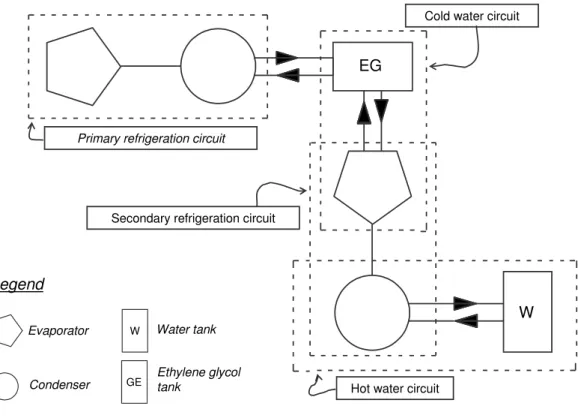
Primary refrigeration circuit
Cold water circuit
Secondary refrigeration circuit
Hot water circuit
EG
W
Evaporator
Condenser
Water tank W
Ethylene glycol tank
GE
Legend
Figure 1 – Schematical of the four parallel circuits experimental facility.
Experimental facilities with no oil contamination are those ones that do not use compressors. It is possible using just gravitational effects to obtain a difference in pressure, but a high difference in level between the evaporator and condenser is required to generate mass flow, which also has the disadvantage of being constant for all experiments.
24 Chapter 1. Experimental setup
refrigeration circuit) is in parallel with an ethylene-glycol circuit (cold water circuit), which is cooled by a heat exchanger interlinked to an evaporator located in a conventional refrigeration system (auxiliary refrigeration circuit) to obtain temperature dropping effect; this auxiliary circuit also uses a cooling tower (or an open circuit of water coming from the supply system), used for cooling (or replace) the water that comes from the condenser’s heat exchanger (hot water circuit). Figure 2 presents a schematic of the four parallel circuits test facility. In case of using three, the cold water circuit will not be used, and the evaporation temperature will be constant for all experiments.
In this work, it is built a refrigeration test facility with four parallel circuits, to take advantage of working at different evaporation temperatures. A magnetically driven micropump was also used in the primary refrigeration circuit to guarantee no oil contamination during the tests. Also, an inverter was used allowing mass flow rate variation.
1.2
Experimental device
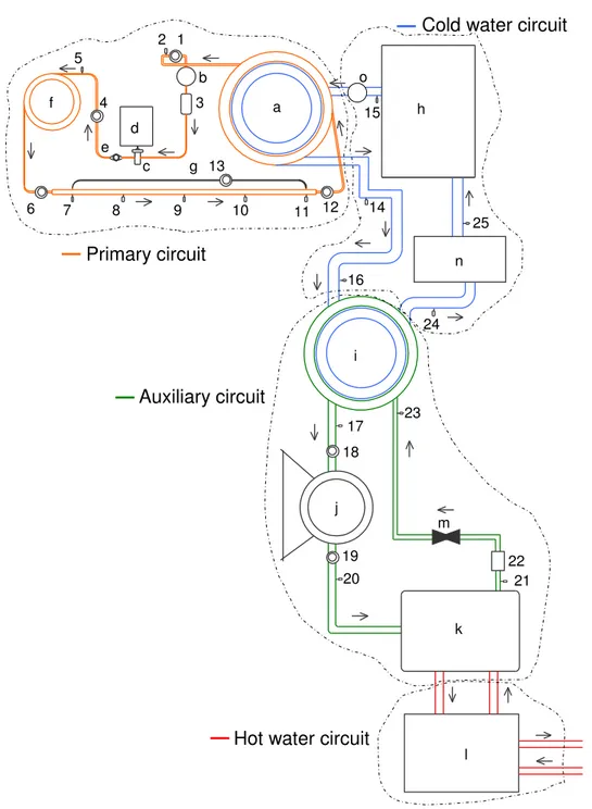
This experimental device is based on the work of Lima (17). Figure 2 presents the experimental facility, highlighting the four parallel circuits, as discussed above. More emphasis will be given to the primary circuit, but more detailed information about the other circuits can be found in Maia (1).
1.2.1
Primary circuit
The primary circuit is comprised of 4 important parts: micropump system, pre-heater, test section and condenser.
The micropump is magnetically driven by a rubber coupling with magnets, con-nected to an electrical motor, generating the mass flow rate required with no oil contam-ination; since there is no contact between mechanical parts, lubrication is not required. Figure3presents a picture showing the components that comprise the micropump system. The magnetic coupling was developed inside the laboratory during the facility assemblage, and it is object of a patent, which is being released by the Federal University of Minas Gerais.
As the system uses a pump instead of a compressor, and there are no expansion mechanisms, the difference in pressure realized during the experiments will be just from friction losses.
1.2. Experimental device 25
2 1
3
c
6
e 5
4
7 8 9 10 11
13
12 14 15
17 16
20
23 24
25
18
19
21 a
b
d f
g
h
i
j
k n
l
22 m
Primary circuit
Cold water circuit
Auxiliary circuit
Hot water circuit o
Figure 2 – Schematical of the experimental facility. In primary circuit, letters: a, condenser; b, liquid bottle; c, micropump; d, electrical motor with inverter; e, butterfly valve; f, pre-heater; g, test section; numbers: 1, 4, 6 and 12, absolute pressure transmitters; 13, differential pressure transmitter; 3, Flow meter; 2, 5, 7 - 11, thermocouples. In cold water circuit, letters: h, ethylene-glycol tank; n, temperature controller; o, pump 2 hp;numbers: 14 - 16 and 25, thermocouples. In auxiliary circuit,
26 Chapter 1. Experimental setup
power output will cause different two phase flow quality. The pre-heater is comprised of a set of 10 resistances with 161 Ω each, arranged in parallel. The equivalent resistance is equal to (10/161Ω)⊗
1 = 16.1 Ω. It is not recommended going over 12.5 A, because it is the maximum value allowed by the varistor’s manufacturer. Figure4shows the Pre-heater and the Varistor during the facility construction.
Magnetic coupling
Micropump Electrical motor
Figure 3 – Motor, coupling and magnetically driven micropump.
Pre-Heater
Varistor
Figure 4 – Pre-heater and varistor.
1.2. Experimental device 27
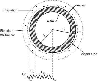
The idea is generating an uniform heat flux on the tube, and after this will be possible determining the heat transfer coefficient (HTC) by using the Newton’s law of cooling and the thermal resistance concept (see Fig. 5):
ℎ= 𝑄˙”
(𝑇𝑤−𝑇𝑠)(𝑟1/𝑟2) −
𝑘 𝑙𝑛(𝑟2/𝑟1)𝑟1
, (1.1)
and,
˙
𝑄′′
= 𝑄
𝑆 =
𝑄
2Þ 𝑟2𝐿
, (1.2)
where ℎ is the HTC (𝑊 𝑚⊗2
𝐾⊗1
), 𝑄′′
is the heat flux (𝑊 𝑚⊗2
), 𝑇𝑤 is the tube internal surface temperature (◇
C), 𝑇𝑠 is the bulk temperature of the fluid (◇C), and 𝑆 is the tube external surface area (𝑚2), 𝑘 is the copper tube thermal conductivity. Heat flux is
considered one-dimensional and in the radial direction.
r1
r2
R1 R
2
Ts
Tw
Q”. Electrical resistance
Insulation
Copper tube
Figure 5 – Determination of the experimental heat transfer coefficient, see Eq.1.1; where,𝑅1=2Þ 𝑟11𝐿 ℎ, and𝑅2=
𝑙𝑛𝑟2 𝑟1
2Þ 𝑘 𝐿.
The condenser is responsible for cooling the refrigerant, in which was heated by the micropump, pre-heater and test section. The total heat exchange required during this process can be determined using Eq.1.3:
˙
𝑄𝑐 = ˙𝑄𝑝ℎ+ ˙𝑄𝑡𝑠+ ˙𝑄𝑚𝑝, (1.3)
where ˙𝑄𝑝ℎ, ˙𝑄𝑡𝑠 and ˙𝑄𝑚𝑝 are the heat transferred by the pre-heater, test section and micropump, respectively, and can be determined as follows:
˙
28 Chapter 1. Experimental setup
and,
˙
𝑄𝑝ℎ=𝐸𝑝ℎΓ𝑝ℎ, (1.5)
and,
˙
𝑄𝑡𝑠 =𝐸𝑡𝑠Γ𝑡𝑠. (1.6)
In this work, it is neglected the micropump contribution, due to its low order of magnitude. During an energy balance should be found that all heat transferred by the condenser’s heat exchanger (see Fig. 2, letter"a"), in the primary circuit side, it is going to the cold water system.
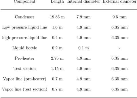
Particularly during the inventory determination, the geometric properties have to be well-defined to obtain accurate results. Table1presents the primary circuit dimensions.
Table 1 – Primary circuit dimensions.
Component Length Internal diameter External diameter
Condenser 19.85 m 7.9 mm 9.5 mm
Low pressure liquid line 1.6 m 4.9 mm 6.35 mm
high pressure liquid line 0.4 m 4.9 mm 6.35 mm
Liquid bottle 0.2 m 0.1 m
-Pre-heater 2.76 m 4.9 mm 6.35 mm
Test section 1.15 m 4.9 mm 6.35 mm
Vapor line (pre-heater) 0.7 m 4.9 mm 6.35 mm
Vapor line (test section) 0.7 m 4.9 mm 6.35 mm
1.2.2
Cold water circuit
Cold water circuit is comprised of a tank with ethylene-glycol at 30% of compo-sition with 70% of water (see Fig. 2, letter "h"), a 2 hp pump and a PID temperature controller (see letter "n"). Looking at the cold water circuit side, the energy balance among points 14 and 15 shows that:
˙
𝑄𝑐 =−𝑄˙𝑝𝑢𝑚𝑝+ ˙𝑚𝑐𝑤𝑐𝑝,𝑐𝑤𝑐∆𝑇𝑐𝑤𝑐 =−𝑄˙𝑝𝑢𝑚𝑝+ ˙𝑚𝑐𝑤𝑐𝑝,𝑐𝑤𝑐(𝑇14−𝑇15), (1.7)
where 𝑄˙𝑐, 𝑄˙𝑝𝑢𝑚𝑝, 𝑚˙𝑐𝑤, 𝑐𝑝,𝑐𝑤𝑐 and ∆𝑇𝑐𝑤𝑐 are the condenser heat transfer rate, cold water
differ-1.2. Experimental device 29
ence for the water, respectively. It is considered ˙𝑄𝑝𝑢𝑚𝑝 negligible since the temperature difference given by this term is lower than the thermocouples uncertainty.
The ethylene-glycol water mass flow rate will be determined indirectly during the experiments, feeding during one minute a recipient, and weighting it using a precision balance, also subtracting the void recipient weight; mass over time spent will give the mass flow rate.
1.2.3
Auxiliary circuit
Auxiliary circuit is a conventional refrigeration system driven by a reciprocating compressor and an expansion mechanism, also using R-134a as refrigerant fluid. Consid-ering a control volume on the evaporator (see Fig. 2, letter "i"), it is possible to obtain the energy balance as:
˙
𝑄𝑐𝑤𝑒= ˙𝑄𝑎𝑐𝑒, (1.8)
and,
˙
𝑚𝑐𝑤𝑐𝑝,𝑐𝑤𝑒(𝑇24−𝑇16) = ˙𝑚𝑎𝑐𝑒(𝑖17−𝑖16), (1.9)
where, 𝑄˙𝑐𝑤𝑒 is the heat transfer rate from the cold water circuit, and 𝑄˙𝑎𝑐𝑒 is the heat
transfer at the R-134a side; 𝑐𝑝,𝑐𝑤𝑒, 𝑇24 and 𝑇16 are the average heat transfer capacity to
the points 24 and 16, temperature at the point 24 and at the point 16, respectively; 𝑚˙𝑎𝑐𝑒
is the R-134a mass flow rate (see the mass flow meter in Fig. 2, number 22), 𝑖16 is the
enthalpy at the evaporator’s inlet (see number 16) and 𝑖17 is the enthalpy at outlet (see
number 17).
1.2.4
Overall energy balance between primary and auxiliary circuits
The water in the cold water circuit is the matter that conveys the energy from the primary to the auxiliary circuit. The steady state is reached when the heat absorbed in the primary circuit and transferred to the auxiliary circuit is the same; and the cold water circuit is used to obtain this equilibrium. And, all system depends on the refrigeration capacity from the auxiliary circuit to reach this balance.
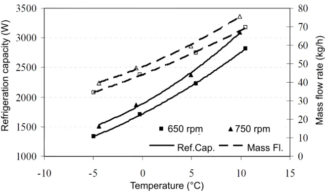
Figure6shows the auxiliary circuit refrigeration capacity (𝑊) in terms of evapora-tion temperature(◇
30 Chapter 1. Experimental setup
Temperature (°C)
R
e
fr
ig
e
ra
ti
o
n
c
a
p
a
ci
ty
(
W
)
M
a
ss
f
lo
w
r
a
te
(
kg
/h
)
650 rpm 750 rpm
Ref.Cap. Mass Fl.
Figure 6 – Refrigeration capacity for the auxiliary circuit in function of evaporation temperature (1), using 50◇𝐶of condensing temperature.
Eq.1.10 presents the overall energy balance between the primary and auxiliary circuits:
˙
𝑄𝑎𝑐𝑒 = ˙𝑄𝑝ℎ+ ˙𝑄𝑡𝑠, (1.10)
where the heat transferred by the micro-pump and cold water pump were not considered; all tubes are considered adiabatic.
1.3
Experimental methodology
The choice of which steps follow during the experiments is made using the flow pattern map as a guide. During the change of pattern, the flow presents a change in saturated liquid distribution around the tube, and this will change the heat transfer as shown in greater details during the literature review section (see item 2). To obtain a data set with a large range of applicability, it is necessary to embrace all types of flow pattern.
The methodology presented by Wojtan et al. (23) was used to generate the Fig.7, that shows a flow pattern map for the R-407C. The conditions used were 15◇
𝐶, 10𝑘𝑊/𝑚2
1.3. Experimental methodology 31
conditions, and volumetric flow in Fig. 7was converted for this condition to facilitate the on-site correlation.
Annular Intermittently dry
Slug
Slug + Stratified wavy
flow wavy flowStratified
Annular Intermittently dry
Slug
Slug + Stratified wavy
flow wavy flowStratified
Stratified flow
M
is
t f
lo
w
Dryout
Figure 7 – Pattern flow map to the R-407C, at 15◇𝐶, 10𝑘𝑊/𝑚2and 20𝑙𝑝ℎ: reference to the water.
For example, considering that the flow meter indicates 20 lph, it means that the fluid could be in the slug pattern, intermittently dry, stratified wavy flow, annular or mist flow, depending on the two-phase quality.
Using the experimental data sets presented in the Tab. 2, it is possible to obtain values for a large range of different conditions, including different types of flow pattern.
Table 2 – Experimental data sets for different operational conditions.
Experiment data set Quality range Heat flux (𝑘𝑊 𝑚⊗2) Volumetric flow (𝑙𝑝ℎ)
1 0.2 to 0.8 6 12, 18, 25
2 0.2 to 0.8 4 12, 18, 25
3 0.2 to 0.8 2 12, 18, 25
Electrical resistances x water in counter current
32 Chapter 1. Experimental setup
along the copper tube on dryout transition region, that hides a peak value of heat trans-fer coefficient nearby, which does not occur when using counter current as the heating mechanism. In this work, electrical resistances are used, and it is not obtained values for the dryout region to avoid this problem.
1.3.1
Uncertainty analysis
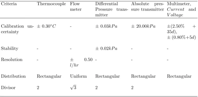
Table 3 presents the calibration uncertainty, stability, resolution and distribution for the measuring instruments installed in the primary circuit and in the cold water circuit. These values will be used to generate the data set of heat transfer coefficient and for the inventory calculation, during the void fraction analysis.
Table4shows the uncertainty for the auxiliary circuit measuring instruments, and it was obtained from Maia (1). These values will be used during the balance of energy to the auxiliary circuit, and calculations that this circuit will be related with.
Table 3 – Uncertainty values for the primary and cold water circuit instruments.
Criteria Thermocouple Flow meter
Differential Pressure trans-mitter
Absolute pres-sure transmitter
Multimeter, 𝐶𝑢𝑟𝑟𝑒𝑛𝑡 and 𝑉 𝑜𝑙𝑡𝑎𝑔𝑒
Calibration un-certainty
±0.30◇𝐶 - ±0.03𝑘𝑃 𝑎 ±20.00𝑘𝑃 𝑎 ±(2.50% +
35𝑑),
±(0.80%+5𝑑)
Stability - - ±0.02𝑘𝑃 𝑎 -
-Resolution - ± 0.50
𝑙/ℎ𝑟
- -
-Distribution Rectangular Uniform Rectangular Rectangular Rectangular
Divisor 2 √3 2 2
Table 4 – Uncertainty values for the auxiliary circuit instruments.
Criteria ThermocoupleFlow meter Absolute pressure transmit-ter for evaporator and con-denser
Calibration uncertainty
±1.64◇𝐶 ±1.35 kg/h ±60𝑘𝑃 𝑎and 370𝑘𝑃 𝑎
1.3. Experimental methodology 33
Methodology used for calculating the uncertainty
Following will be presented an example to demonstrate how the uncertainty is calculated for each one of pressure and temperature measurements.
Consider a thermocouple and an absolute pressure transmitter located in the test section. During steady state, it is recorded 45 measurements of temperature and pressure during one minute, as shown by Fig. 8. It is observed some expected variability, and this variability is taken into account during the expanded uncertainty calculation, as will be shown below.
0 20 40 60
13.2 13.3 13.4 13.5 13.6 13.7 13.8 T e m p e a rt u re [ C e lsi u s]
nº measurements [-] 0 20 40 60
670 680 690 700 710 720 730 740 P re ssu re [ kP a ] nº measurements
Figure 8 – Measurements of temperature and pressure, showing an example of the variability presented during the steady state experiments in the test section.
First step is obtaining an average for the 45 measurements presented in the Fig.8, as shown by Eq. 1.11:
¯
𝑇 =
𝑁 ∑︀ 𝑖=1𝑇𝑖
𝑁 = 13.51
◇ 𝐶, ¯ 𝑃 = 𝑁 ∑︀ 𝑖=1𝑃𝑖
𝑁 = 711.17𝑘𝑃 𝑎,
(1.11)
and, the standard deviation can be determined as:
𝑠𝑇 = ⎯ ⎸ ⎸ ⎸ ⎷ 𝑁 ∑︀ 𝑖=1(𝑇𝑖−
¯ 𝑇)2
𝑁 = 0.1
◇
𝐶,
𝑠𝑃 = ⎯ ⎸ ⎸ ⎸ ⎷ 𝑁 ∑︀ 𝑖=1(𝑃𝑖−
¯ 𝑃)2
𝑁 = 14.12𝑘𝑃 𝑎.
34 Chapter 1. Experimental setup
Standard uncertainty is obtained dividing the standard deviation by the root square of the number of measurements, using the equation below:
𝑢1(𝑇) = 0.1
◇
𝐶/√45 = 0.015◇
𝐶,
𝑢1(𝑃) = 14.12𝑘𝑃 𝑎/
√
45 = 2.10𝑘𝑃 𝑎. (1.13)
The calibration uncertainty is presented by the manufacturer multiplied by the coverage factor of 2. To correct this expanded uncertainty to obtain the standard uncer-tainty:
𝑢2(𝑇) = 0.3
◇
𝐶/2 = 0.15◇
𝐶,
𝑢2(𝑃) = 20 𝑘𝑃 𝑎/2 = 10.06𝑘𝑃 𝑎.
(1.14)
The combined uncertainty is obtained using a summation in quadrature of the standard uncertainty presented in Eq. 1.14, plus the calibration uncertainty presented in the Table3:
𝑢𝑐(𝑇) = √︁𝑢1(𝑇)2+𝑢2(𝑇)2 =
√
0.015◇𝐶2+ 0.15◇𝐶2 = 0.15◇𝐶,
𝑢𝑐(𝑃) =√︁𝑢1(𝑃)2+𝑢2(𝑃)2 =
√︁
(2.1𝑘𝑃 𝑎)2+ (10𝑘𝑃 𝑎)2 = 10.22𝑘𝑃 𝑎. (1.15)
The degrees of freedom for these measurements are calculated as below:
𝑣𝑒𝑓(𝑇) =
𝑢𝑐(𝑇)4
𝑢1(𝑇)4
𝑣T +
𝑢2(𝑇)4 ∞
= 0.15
◇
𝐶4 0.015◇𝐶4
45⊗1 +
0.15◇𝐶4 ∞
= 408738,
𝑣𝑒𝑓(𝑃) =
𝑢𝑐(𝑃)4
𝑢1(𝑃)4
𝑣P +
𝑢2(𝑃)4 ∞
= 10.06𝑘𝑃 𝑎
4 2.10𝑘𝑃 𝑎4
45⊗1 +
10.06𝑘𝑃 𝑎4 ∞
= 24464,
(1.16)
where𝑣𝑇 and𝑣𝑃 are the degree of freedom for the temperature and pressure, respectively. They are obtained from the number of measurements (45) minus one, for both temperature and pressure. Table5gives the coverage factor 𝑘95, using the effective degrees of freedom
(𝑣𝑒𝑓) obtained from Eq.1.16. For higher values of degrees of freedom as shown in Eq.1.16, the coverage factor will be approximately 2, representing a confidence level of 95%, and the expanded uncertainty will be determined as:
Table 5 – Student t-factor to determine the coverage factor for a level of confidence of 95%.
𝑣𝑒𝑓 1 2 3 4 5 6 7 8 10 20 50 100 ∞
𝑘95 13.97 4.53 3.31 2.87 2.65 2.52 2.43 2.37 2.28 2.13 2.05 2.02 2
𝑢𝑐(𝑇)95% =𝑢𝑐(𝑇)𝑘95(𝑇) = (0.15
◇
𝐶)·(2) = 0.3◇
𝐶,
𝑢𝑐(𝑃)95% =𝑢𝑐(𝑃)𝑘95(𝑃) = (20.11𝑘𝑃 𝑎)·(2) = 20.12𝑘𝑃 𝑎.
1.4. Validating the test section quality and energy balance at the pre-heater 35
And, the temperature and pressure can be finally expressed as:
𝑇 =𝑇¯±𝑢𝑐(𝑇)95% = 13.51 ◇𝐶±0.3◇𝐶,
𝑃 = ¯𝑃 ±𝑢𝑐(𝑃)95% = 711.17𝑘𝑃 𝑎±20.12𝑘𝑃 𝑎.
(1.18)
It is possible to conclude that the results presented high precision, and the ex-panded uncertainty is basically the calibration uncertainty multiplied by the coverage factor.
For flow meter and multimeter, just one measurement was taken during the ex-periments; also, the resolution must be taken into the account. The standard uncertainty will be equal to the resolution over the cube root, plus the calibration uncertainty, using Eq. 1.14, Eq.1.15, Eq. 1.17 and Eq. 1.18, as used here for temperature and pressure.
Software EES was used to calculate the uncertainty propagation, and the method-ology implemented can be seen in the EES’s manual (27).
1.4
Validating the test section quality and energy balance at the
pre-heater
As R-407C is a zeotropic fluid, it is not necessary calculating the quality using an energy balance for the pre-heater and test section, as required for a pure fluid. The thermodynamic state inside the test section can be determined just using the temperature and pressure measurements in the test section. On the other hand, in order to validate thermodynamic state in the test section, values of quality using both methodologies can be correlated.
The quality can be calculated using a control volume on the pre-heater, by the following energy balance Eqs.1.19 and 1.20:
˙
𝑄𝑝ℎ = ˙𝑚𝑅407𝑐 ∆𝑖𝑝ℎ = ˙𝑚𝑅407𝑐 (𝑖7 −𝑖5)∴𝑖7 =𝑖5+ ˙ 𝑄𝑝ℎ
˙ 𝑚𝑅407𝑐
, (1.19)
and,
𝑥1 =
𝑖7 −𝑖𝑙
𝑖𝑣 −𝑖𝑙
, (1.20)
36 Chapter 1. Experimental setup
the state equations for R-407C, as a function of quality and𝑃6:
𝑖𝑙 =𝑓(𝑥= 0, 𝑃6),
𝑖𝑣 =𝑓(𝑥= 1, 𝑃6).
(1.21)
An alternative method to calculate the quality by Eq. 1.20 is using the state equations for the R-407C, in function of𝑇7 and 𝑃6:
𝑥2 =𝑓(𝑇7, 𝑃6). (1.22)
Comparing 𝑥1 and 𝑥2 is possible to validate the quality in the test section. Also,
it is possible to determine which method has the lower uncertainty. For example, an experiment was made using the following properties:
• 𝑇5 = (10.96±0.31)◇𝐶,
• 𝑃4 = (817.28±20.88)𝑘𝑃 𝑎,
• 𝑇7 = (13.54±0.31)◇𝐶,
• 𝑃6 = (816.65±20.95)𝑘𝑃 𝑎,
• 𝑚˙𝑅⊗407𝐶 = (25±0.5)𝑙𝑖𝑡𝑒𝑟𝑠/ℎ𝑟,
and, the results obtained were:
• 𝑥1 = 0.2274±0.01011,
• 𝑥2 = 0.2176±0.1278.
First, the results show that the energy balance in the pre-heater is well satisfied; second, these results demonstrate that the uncertainty is higher when using the tem-perature 𝑇7 as a source, because a low variation in the temperature can cause a larger
propagation during the uncertainty calculation, because of the glide. Following, it will be shown a section to present the main characteristics of the refrigerant fluid used in this work, the R-407C.
1.5
Refrigerant fluid R-407C
1.5. Refrigerant fluid R-407C 37
DuPont™ Suva® 407C
Pressure-Enthalpy Diagram
(SI Units)
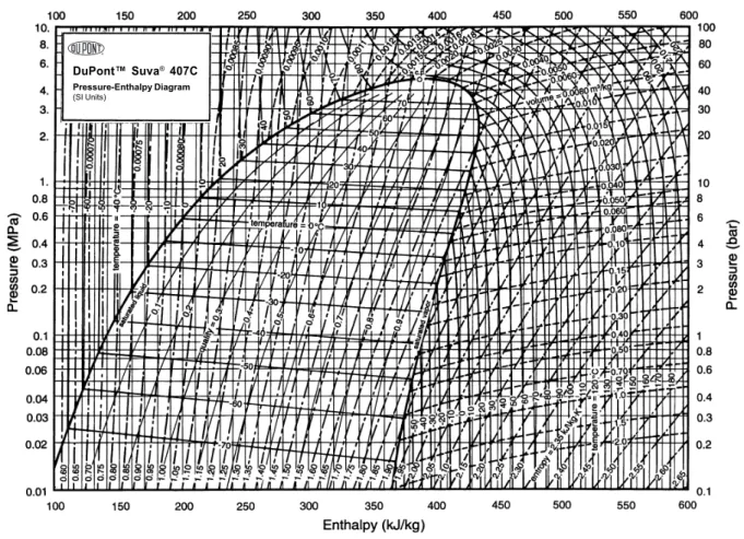
Figure 9 – Pressure versus Enthalpy diagram for the R-407C.
and 52%, respectively, containing no ozone-depleting chlorine. Figure9shows a pressure-enthalpy diagram for the R-407C, provided by the manufacturer DuPont.
A zeotropic mixture is that one in which temperature change is observed at con-stant pressure during phase change. Latini (28) classifies a fluid as zeotropic if this temperature variation is greater than 5◇
𝐶. Zeotropic fluids also have the quality of being distillable, and also the proportion between the fluids can change inside the refrigeration system depending on the thermodynamic state. Another important issue occurs during recharge, because it is difficult predicting the exactly amount of fluid inside the system, and the composition of this one. R-407C is indicated as one of the most important candidate to replace the R-22, because they have similar properties at operational points.
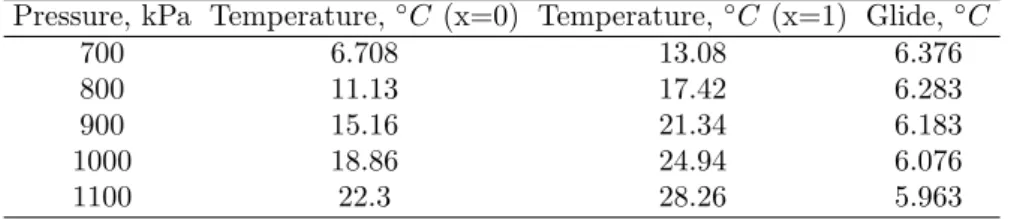
Looking at Table 6, it is possible to see the relation between pressure, saturation temperature and glide for the R-407C. In this work, the test section pressure will range between 700kPa to 1100kPa, which means that the temperature will vary between 6.7◇
𝐶
to 28.96◇
𝐶, and the glide will be approximately constant, equals to 6◇
𝐶. In consequence of this glide, the evaporation temperature will increase along the test section, and this relation is considered linear, ∆𝑇 = 6◇
𝐶∆𝑥; for example, considering ∆𝑥= 1%, ∆𝑇 will be 0.06◇
𝐶. Considering that the absolute uncertainty is equal to approximately 0.3◇
38 Chapter 1. Experimental setup
will be difficult to realize quality changes for less than 5%, accurately.
Table 6 – Glide to be observed for the pressure range used during the experiments.
Pressure, kPa Temperature,◇𝐶(x=0) Temperature,◇𝐶 (x=1) Glide,◇𝐶
700 6.708 13.08 6.376
800 11.13 17.42 6.283
900 15.16 21.34 6.183
1000 18.86 24.94 6.076
1100 22.3 28.26 5.963
1.6
Conclusion
Part II
41
2 Methodology and literature review
2.1
Literature review on coefficient of heat transfer relations
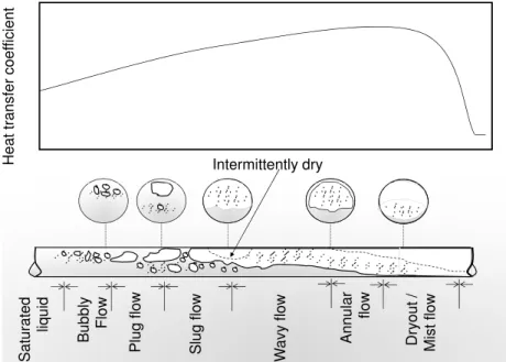
Understanding the different phase change flow regimes is critical to the develop-ment of HTC correlations. Phase changing has multiple roles in HVAC, and what is particularly relevant in our study is the enhancing mechanism for heat transfer capacity. In general, heat transfer rates during phase change can be 4 to 25 times higher than for equivalent single-phase forced convection (29). Figure 10describes the most relevant flow patterns and HTC levels during the phase change process along an evaporator tube. The flow pattern presented in this figure is only illustrative and it will vary depending on the fluid characteristics and flow regimes (evaporation temperature, vapor pressure, heat flux, mass flow velocity, diameter and vapor quality, etc.) Observing the evolution of HTC regimes along the evaporator it is possible to recognize:
• a gradual increase in HTC due to the phase change phenomena, related to nucleate and convection boiling;
• a rapid decrease for high values of quality, more precisely in the region identified as dryout/mist flow.
The phase change mechanism can be further divided into two different processes: convection boiling, which is the phase change regime that occurs in the liquid/vapor
inter-H e a t tr a n s fe r c o e ff ic ie n t Intermittently dry S a tu ra te d liq u id A n n u la r fl o w B u b b ly F lo w P lu g f lo w S lu g f lo w W a v y f lo w D ry o u t / M is t fl o w
42 Chapter 2. Methodology and literature review
face, and nucleate boiling, which is the phase change regime related to bubble formation on a heated surface (liquid/solid interface). There is a group of correlations, called Strictly Convective, that considers only the convection term during the calculation of a two-phase flow HTC (30, 31, 32,33,34,35,36). In general, Strictly Convective correlations use the well-known Dittus-Boelter heat transfer relation applied to saturated liquid flow and the Martinelli parameter (37), as expressed by:
ℎ𝑡𝑝 =ℎ𝑙(1 +𝐶𝑙ä𝑡𝑡)
⊗𝐶2
, (2.1)
where𝐶1 and 𝐶2 are constants obtained empirically, as proposed by Bandarra (36).
An-other group of correlations, called Superposition Rule correlations, considers both pro-cesses: convection boiling (ℎ𝑐𝑏) and nucleation boiling(ℎ𝑛𝑏) (38, 4, 39, 6, 40, 41). These correlations determine the functional form of the HTC by weighing the contribution of each mechanism of heat transfer (ℎ𝑛𝑏 and ℎ𝑐𝑏) as:
ℎ𝑡𝑝 = [(𝐹 ℎ𝑐𝑏)𝑛+ (𝑆ℎ𝑛𝑏)𝑛]1/𝑛. (2.2)
In Eq. 2.2 the factors 𝑆 and 𝐹 are weighing factors for the two components. At high values of mass flow, the temperature gradient near the wall increases as consequence of a thinner boundary layer. The effective temperature around bubbles also decreases reducing the chances of new bubble formation. In this situation the suppression factor 𝑆
becomes smaller. Likewise at high vapor quality flow regimes there is a smaller chance of bubble formation, and the suppression factor𝑆 should again decrease. Otherwise, the convective heat transfer should increase for high values of quality and mass flow, and the factor𝐹, composed by the Martinelli parameteräshould express it. When the parameter
𝑛is not equal to unity, the weighing is biased, and the result tends to become closer to the largest value among the two terms. Generally speaking, Superposition Rule correlations produce more robust and useful approximations than Strictly Convective correlations.
A third group of two-phase flow approximations for HTCs is the so-called Strictly Empirical (42,5,43). In this group dimensionless numbers are correlated to experimental data using numerical methods for optimization of the coefficients. This technique has gained popularity (44, 45) with the increase of computational power in recent years that enables testing large quantity of dimensionless numbers and increasingly complex data sets.
2.1. Literature review on coefficient of heat transfer relations 43
determination (48) has been greatly mitigated by new methodologies, as presented by Ursenbacher et al. (49). The main drawback of using Wojtan et al. (23,26) methodology is the assumption of 𝑎 𝑝𝑟𝑖𝑜𝑟𝑖 knowledge of the heat flux, which is typically what the designer is trying to determine in the first place.
In this work is tested different correlations to verify which one will predict better the HTC for the R-407C.
550 500 M ist fl o 500 450 400 Intermittently dry 2.s -1] flo w D ryo u t 400 350 Annular Slug u x [kg .m -2. 300 250 Slug M a ss fl u
x 250
200
Slug + Stratified wavy
flow Stratified wavy flow M 150 100 wavy flow Stratified flow 50 0
Quality [ - ]
0 0.1 0.2 0.3 0.4 0.5 0.6 0.7 0.8 0.9 1 0
Figure 11 – Flow pattern map for refrigerant R-22 for saturation temperature of 8◇C, an internal diameter
of 12.97 mm, and heat flux of 5 𝑘𝑊 𝑚⊗2.
2.1.1
Heat transfer coefficient relations used in this work
The relations of Kandlikar (5), Gungor and Winterton (4) and Watellet (6) were used to test the correlation with the experimental data, and these relations can be found in Tab. 7.
44 Chapter 2. Methodology and literature review
Table 7 – Heat transfer coefficient relations used in this work.
Author Correlation
Kandlikar (5) ℎ𝑡𝑝=ℎ𝑙 ⎦
𝐶1𝐶𝑜𝐶2(25𝐹 𝑟𝑙)𝐶5+𝐶3𝐵𝑜𝐶4𝐹𝑓 𝑙 ⎢
Convective region: 𝐶=
⎦
1.136,−0.9,667.2,0.7,0.3
⎢
Nucleate boiling region: 𝐶=
⎦
0.6683,−0.2,1058.0,0.7,0.3
⎢
𝐹𝑓 𝑙= 2.2, considered the same as R-22
Gungor and Winterton (4) ℎ𝑡𝑝=ℎ𝑙 ⎦
1 + 3000𝐵𝑜0.86+ 1.12( 𝑥 1⊗𝑥)
0.75(𝜌𝑙
𝜌𝑣)
0.41 ⎢
Watellet (6) ℎ𝑡𝑝= (ℎ2𝑒𝑐.5+ℎ2𝑛𝑏.5)⊗2.5, where, 𝐹𝑤= 1 + 1.925ä⊗𝑡𝑡0.83
if𝐹 𝑟𝑙≤0.25,𝑅𝑤= 1.32𝐹 𝑟𝑙0.2
if𝐹 𝑟𝑙>0.25,𝑅𝑤= 1 ℎ𝑒𝑐=𝐹𝑤𝑅𝑤ℎ𝑙
Parameters used in common: ℎ𝑙= 0.023𝑅𝑒𝑙0.8𝑃 𝑟0𝑙.4𝑘𝑑𝑙 𝑅𝑒𝑙=𝐺Û𝑑𝑙(1−𝑥)
ℎ𝑛𝑏= 55(𝑃𝑟)0.12(−𝑙𝑜𝑔10(𝑃𝑟))⊗0.55𝑀⊗0.5(ã)0.67
2.2
Methodology to obtain general heat transfer coefficient
rela-tions for pure and azeotropic fluids
This section describes the methodology used to generate the new correlations. The first step in this process is to create a set of inputs that may or may not be included in the correlations. The first group of inputs takes the form of dimensionless numbers based on several properties 𝑑, 𝑈, 𝑘, Û and 𝑖𝑙𝑣, and are determined through the Buckinham’s Π theorem (50). Other inputs consist of the enhancing factor 𝑆 presented in Lima (17) (see correlation number 4, Tab. A.1), and the dimensionless numbers given by Wojtan et al. (23,26). The parameters𝐶1,𝐶2 to𝐶5are also used here in order to consider the influence
2.2. Methodology to obtain general heat transfer coefficient relations for pure and azeotropic fluids 45
correlations are given by:
ℎ𝑡𝑝 =
⎠∑︁𝑛1
𝑖=1
𝑎𝑖𝑋𝑖𝑏i
⎜⎠∏︁𝑛2
𝑗=1
𝑋𝑐j
𝑗 ⎜
, (2.3)
and,
ℎ𝑡𝑝=𝑎0
𝑛1
∑︁
𝑖=1
𝑎𝑖𝑋𝑖𝑏i+𝑐0
𝑛2
∏︁
𝑗=1
𝑋𝑐j
𝑗 , (2.4)
where the 𝑋’s are a subset of the dimensionless parameters in Tab. A.1, and the coeffi-cients 𝑎𝑖, 𝑏𝑖 and 𝑐𝑗 can be negative which means that these expressions can also include subtractions and divisions.
The third functional form is based on the Superposition Rule:
ℎ𝑡𝑝 =
⎟⎞
𝑎0
𝑛1
∑︁
𝑖=1
𝑎𝑖𝑋𝑖𝑏i+𝑐0
𝑛2
∏︁
𝑗=1
𝑋𝑐j
𝑗 ⎡
ℎ𝑛𝑙]
+⎞𝑎0
𝑛1
∑︁
𝑖=1
𝑎𝑖𝑋𝑖𝑏i+𝑐0
𝑛2
∏︁
𝑗=1
𝑋𝑐j
𝑗 ⎡
ℎ𝑛 𝑛𝑏
⟨1/𝑛
,
(2.5)
where ℎ𝑙 is the correlation of Dittus-Boelter applied for saturated liquid flow and ℎ𝑛𝑏 is the nucleate boiling HTC correlation presented by Cooper (51).
For a given set of𝑋 the correlation’s coefficients𝑎𝑖,𝑏𝑖 and𝑐𝑗 are determined using an unconstrained line-search method (52) implemented in Matlab R2012b and accessible through the Optimization toolbox via the function 𝑓 𝑚𝑖𝑛𝑢𝑛𝑐. The optimization method searches for the coefficients that minimize the root mean squared error (RMSE) between the experimental HTC and Eq. 2.3, 2.4 and 2.5.
The fourth type of correlation considered is obtained through ANNs. ANNs are useful tools for approximating complicated mapping functions for problems in classifica-tion and regression (53) and have been used extensively in many areas. The advantage of ANNs is that no assumptions are required about the underlying process relating input and output variables. However, because ANNs are universal approximating functions, their mapping capabilities can potentially lead to problems such as over-fitting training data (53), and thus leading to poor generalization on new data sets. In this study the ANN is a representation of HTC in terms of a subset of the dimensionless parameters𝑋. The ANN representation is based on signals being sent through elements called neurons in such a way that the processing of the inputs signals produces an output HTC or target value which in this case, are the experimental values for HTC. Neurons are arranged in layers, where the first layer contains the set of inputs, the last layer contains the output, and the layers in between (referred to as hidden layers) contain hidden neurons. The feedforward neural network that is used here, with 𝑁𝑖 inputs and𝑁ℎ neurons in one hidden layer and linear output activation function, can be expressed as
ℎ𝑡𝑝 =𝑎0
⎟𝑁
h
∑︁
𝑖=1
𝑤𝑖𝑓ℎ
⎠ 𝑁
i
∑︁
𝑗=1
𝑤𝑖𝑗𝑋̃︁𝑗 +𝑤𝑖0
⎜ +𝑤0
⟨
46 Chapter 2. Methodology and literature review
where 𝑓ℎ
𝑖 is a transfer function and 𝑋̃︁𝑗 is the 𝑗th dimensionless parameter normalized in the range [−1,1] using the range limits listed in Table A.1. Numerical optimization algorithms such as back-propagation, conjugate gradients, quasi-Newton, and Levenberg-Marquardt have been developed to efficiently adjust the weights,𝑤𝑖 and 𝑤𝑖𝑗 and bias 𝑤𝑖0
and 𝑤0 in the feedforward neural network seeking to minimize a performance function
like the mean squared error.
Table A.1 – Input parameters considered in the search for HTC correlations
𝑋𝑖 Relation Source Range 𝑋𝑖 Relation Source Range
1 𝑅𝑒𝑙,1=𝐺(1−𝑥)Û𝑑𝑙 [83,33870] 15 𝑃8=𝑑𝑖0𝑙𝑣.5 𝜌𝑣
Û𝑒𝑞
[30]
[3×10⊗3,5×10⊗2]
2 ä𝑡𝑡= (1⊗𝑥𝑥 )0.875
(𝜌𝑣
𝜌𝑙)
0.5(Û𝑙
Û𝑣)
0.125
[1.8,118.6] 16 𝑃9=𝑖𝑑𝑔0.5
𝑙𝑣 [4.9×10
5,107]
3 𝐹 𝑟𝑙= 𝐺
2
𝜌2 𝑙𝑔 𝑑
[29] [0.01,1.6] 17 𝑃10=𝑈𝑈𝑣𝑙 [6.4×10⊗7,8×10⊗7]
4 𝑈 𝐶1=
1 + 1.893ä⊗0.77 𝑡𝑡
[4.7×10⊗3,3.0] 18 𝐶
1=𝑃𝑐𝑟𝑖𝑡𝑃 [0.09,0.2]
5 𝑅𝑒𝑙,2=𝜌𝑙𝑈𝑙Û𝑑𝑒𝑞 [4.5×103,2.5×105] 19 𝐶2=𝜌𝑐𝑟𝑖𝑡𝜌𝑣 [0.03,0.1]
6 𝑃 𝑟𝑒𝑞=Û𝑒𝑞𝑐𝑝𝑘𝑒𝑞𝑒𝑞 [2.5×10⊗4,11.1] 20 𝐶3=𝜌𝜌𝑐𝑟𝑖𝑡𝑒𝑞 Present [0.18,2.7]
7 𝑃1=𝑈𝑖𝑙𝑣2 𝑙
[7.7×105,1.4×108] 21 𝐶
4=𝜌𝑐𝑟𝑖𝑡𝜌𝑣 work [2.1,2.75]
8 𝑃2=𝑈𝑙àÛ𝑒𝑞 [119.5,7084] 22 𝐶5=𝑇𝑐𝑟𝑖𝑡𝑇𝑙 [0.06,0.16]
9 𝑅𝑒𝑙,3=𝜌𝑙𝑈𝑣Û𝑑𝑒𝑞 [27.8,70.2] 23 𝜖= 𝑥
𝜌𝑣{[1 + 0.12(1−𝑥)](
𝑥 𝜌𝑣+
1⊗𝑥 𝜌𝑙 ) +
1.18(1⊗𝑥)[𝑔à(𝜌𝑙⊗𝜌𝑣)] 0.25
𝐺𝜌0.5
𝑙 }
⊗1
[0.46,1]
10 𝑃3=𝑈𝑑𝑔2
𝑙 [30] [1.8×10
5,1.2×107] 24 𝑥
𝐼𝐴={[0.291(𝜌𝜌𝑣𝑙)⊗0.571
(Û𝑣
Û𝑙)
⊗0.143] + 1}⊗1
[26] [0.32,0.43]
11 𝑃4=𝑑𝑖
0.5 𝑙𝑣𝜌𝑙
Û𝑒𝑞 [0.62,9.0] 25 𝑄𝑐𝑟𝑖𝑡=
0.131𝜌0.5
𝑣 𝑖𝑙𝑣[𝑔à(𝜌𝑙⊗𝜌𝑣)] 0.25
𝑊 𝑚−2
[3.6×105,4.75×105]
12 𝑃5=𝑖𝑈0.𝑙5
𝑙𝑣 [3.3×10
7,3.3×108] 26 𝐵𝑜= ã
𝐺𝑖𝑙𝑣 [29] [5×10
⊗5,1.3×10⊗5]
13 𝑃6=𝑖0.5à
𝑙𝑣Û𝑒𝑞 [8.6×10
⊗5,1.1×10⊗3] 27 ℎ
𝑙= 0.023𝑅𝑒0𝑙.8𝑃 𝑟𝑙0.4 𝑘𝑙
𝑑 [7,943]
14 𝑃7=𝑖𝑈0.𝑣5 𝑙𝑣
[0.1,1] 28 ℎ𝑛𝑏=
55𝑃0.12
𝑟 (−𝑙𝑜𝑔𝑃𝑟)⊗0.55× 𝑀⊗0.5𝑞0.67
[31] [1180,4377]
The correlations given by these expressions are uniquely determined by the inputs
2.2. Methodology to obtain general heat transfer coefficient relations for pure and azeotropic fluids 47
the second in the range [1,4] is used to select the transfer function𝑓ℎ out of 4 possibilities: hyperbolic tangent sigmoid transfer function, log-sigmoid transfer function, radial basis transfer function or the linear transfer function.
The best correlation for each one of the for types here explored is be the one one that minimizes the RMSE:
argmin ⃗ 𝑥
⎯ ⎸ ⎸
⎷1
𝑁
𝑁 ∑︁
𝑖=1
⎞
ℎ𝑡𝑝,𝑒𝑥𝑝,𝑖−ℎ𝑡𝑝,𝑖(⃗𝑥)
⎡2
, (2.7)
where ℎ𝑡𝑝,𝑒𝑥𝑝 is the experimental HTC, and ℎ𝑡𝑝 is the HTC computed by the new corre-lations defined by the vector ⃗𝑥.
The minimization problem given by Eq. 2.7 is achieved with a genetic algorithm (GA). Gradient-based optimization methods are not suited for this problem because it is not trivial to compute the gradient of Eq. 2.7 with respect to ⃗𝑥. The GA is a space search technique based on the mechanism evolution and survival of the fittest (54). In this algorithm the evolution starts with a population of individuals (determined by vectors
⃗𝑥). Each individual in the population is ranked according to the RMSE Eq. 2.7, between the experimental and the calculated HTC values. The initial population is evolved based on the selection, crossover and mutation operators with the objective to minimize RMSE. Crossover operates on individuals (parents) determined by the selection operator that selects individuals for crossover based on fitness. In this method is used the stochastic uniform methods to select individuals for crossover, in this method the probability of selection is proportional to the individuals’ fitness. Crossover recombines the genetic material of the selected parents. This method uses the scattered method in which a random binary vector with the same length as 𝑋⃗ is used to select the elements coming from each parent. The crossover operator selects elements from the first parent where the vector has 0 entries and selects genes from the second parent when it has 1 entry. The mutation operator modifies individuals that have not been selected for reproduction by randomly changing ⃗𝑥. In this method is used the uniform mutation algorithms that selects a fraction of the vector⃗𝑥for mutation and each of these entries has a 5% probability mutated. If the entry is mutated, each selected entry is replaced by a uniformly random entry. Once the population for a new generation is determined this process continues until some criterion is met. Given that it is difficult to formally specify a convergence criterion for the genetic algorithm due to its stochastic nature, and the algorithm stops after 100 generations or if no improvement has been observed over a pre-specified number of generations, in this case 50, whichever happens first.
2.2.1
HTC zeotropic degradation
48 Chapter 2. Methodology and literature review
phase change, the more volatile fluid becomes vapor first and at a higher velocity rate than the less volatile, and as consequence of this fact the saturate liquid becomes richer in a higher boiling point fluid; this change on the liquid fraction composition of the mixture causes an increase on the wall superheating for the same heat flux, causing a decreasing on the HTC. According Venter (55) the degradation becomes more pronounced for higher pressure and heat flux, and for a determined concentration in the equilibrium of phases. Several authors have been studying the degradation on nucleate boiling HTC in mixtures (55, 2, 56, 57, 58, 59,60, 61, 62,63, 64, 65, 66,67, 68, 69).
Schlindwein et al. (69) more recently have used a methodology in which a reduction factor is applied on the HTC pure fluid relation to obtain the HTC relation for mixtures. The reduction factor applied on the nucleate boiling has the following functional form:
ℎ𝑛𝑏,𝑚
ℎ𝑛𝑏,𝑝
= 1
1 +𝐾, (2.8)
where,ℎ𝑛𝑏,𝑚 is the mixture nucleate boiling HTC, ℎ𝑛𝑏,𝑝 is the pure fluid nucleate boiling HTC, and K is the reduction factor. The same methodology will be applied in this work.
Lee et al. (2) indicate that the temperature profile in a mixture is different from a pure refrigerant, and this difference was presented as depicted in Fig. 12. Lee et al. proposed using this approach to take into account the degradation effects. A reduction factor was proposed:
ℎ𝑚 =
ℎ𝑝 1 +𝐾 =
ℎ𝑝
1 + ℎpure(𝑇int⊗𝑇l)
˙
𝑄”
, (2.9)
and,
𝑇𝑖𝑛𝑡=𝑇𝑣−(1−𝑥)(𝑇𝑣−𝑇𝑙), (2.10)
where 𝑇𝑖𝑛𝑡 is the temperature at liquid/vapor interface; ℎ𝑝 is the HTC calculated by relations developed for a pure fluid andℎ𝑚 is the HTC corrected for mixtures.
Looking at Eq. 2.9 and Eq. 2.10 is possible to see that the correlation proposed by Lee et al. (2) applies the reduction factor to the overall HTC (convective and nucleate boiling), and does not do it just for nucleate boiling as indicated by Schlindwein et al. (69). Also, this relation was proposed for condensation, and this present work is applied for evaporation phenomenon.
Gorenflo (56) presented a review on pool boiling, showing aspects related to the degradation caused by mixtures on nucleate boiling HTC. A reduction factor is applied as below:
𝐾 =
⎠
𝑇𝑖𝑛𝑡−𝑇𝑠 ⎜
2.2. Methodology to obtain general heat transfer coefficient relations for pure and azeotropic fluids 49
Center line
Heat flux
Tv Tv
Tsat
Tw T
w
Vapor
Tint
Copper tube Liquid
Mixture refrigerant Pure refrigerant
Figure 12 – Comparison between the temperature profile in a pure refrigerant and in a mixture according (2).
and,
∆𝑇𝑖𝑑 = ˙𝑄”/ℎ𝑛𝑏,𝑝, (2.12)
and,
∆𝑇𝑖𝑑 = ∑︁
𝑥𝑗∆𝑇𝑗, (2.13)
and,
𝑇𝑖𝑛𝑡−𝑇𝑠 ≈ ∑︁
𝑇𝑠𝑗(𝑥𝑗 −𝑦𝑗)(1−𝑒𝑥𝑝(−𝐵𝑄˙”/𝜌Ñ∆ℎ𝑙𝑣)), (2.14)
where𝑥and𝑦are the molar fraction of liquid or vapour,Ñ is the mass transfer coefficient,
𝜌 and ∆ℎ𝑙𝑣 are density and heat of vaporization, and 𝐵 is a fitting parameter, and Ñ is the mass transfer coefficient.
Thome (57) proposed the following approximation:
𝐾 = ℎ𝑛𝑏,𝑝˙
𝑄” ∆𝑇𝑏𝑝 ⎠
1−𝑒𝑥𝑝 −𝑄˙” 𝜌𝑙ℎ𝑙𝑣Ñ
⎜
, (2.15)