Abstract
A modified three-phase composite model yielding reliable effec-tive characteristics of composite structures has been proposed. In particular, the problem of effective heat transfer coefficient of the composite structure with periodically located inclusions of circu-lar cross-sections located on a square net is solved. Advantages of the proposed model in comparison to the classical three-phase model are illustrated and discussed.
Keywords
Composite, three-phase model, periodic inclusions, heat transfer
Application of an improved three-phase model to calculate
effective characteristics for a composite with cylindrical inclusions
1 INTRODUCTION
The three-phase model of a composite (TPhM) has been used in references [2-5,10,11,15-17] in order to define effective characteristics of composite structures. The physical meaning of the idealization introduced by TPhM relies on substitution of the periodic structure being studied by its counter-part homogeneous homogenized structure with the equivalently reduced parameters (to be defined) except of only one characteristic structure cell. Further step of the solution requires derivation of mathematical formulas regarding homogenized coefficients through the application of physical un-derstanding and mainly via either the energy principle [4,5,10,11,17] or structure geometry [2,3,15,16].
In particular, in the problem devoted to determination of the equivalent heat transfer coefficient of a two-phase composite structure with periodic cylindrical inclusions of circular cross-sections lo-cated on a square net the analysis revealed the following essential features:
(i) For small inclusions size a 1 heat transfer parameter is validated for its arbitrary val-ues;
(ii) For large inclusion size a 1 the TPhM model yields reliable results assuming that heat
transfer of the inclusions is of the order of structure matrix ~ 1 ;
Igor V. Andrianov1, Jan Awrejcewicz2, Galina A. Starushenko3
1 Institute of General Mechanics, RWTH Aachen University, Templergraben 64, D-52056, Aachen, Germany
2 Technical University of Łódź, Department of Aut o-mation and Biomechanics, 1/15 Stefanowski St., PL-90-924, Łódź, Poland
3 Dnipropetrovs’k Regional Institute of State Manag e-ment of National Academy of State Managee-ment at the President of Ukraine, Gogolya 29, UA-49631,
(iii) PhM may yield even a qualitatively wrong result for either large inclusion size a 1 or
large/small conductivity properties, i.e. for and 0.
A construction of the first order TPhM approximation using the method of variations of bound-ary shapes of the studied structure does not allow us to overcome the earlier mentioned problems, in particular with respect to the possible wide spectrum of applications. Furthermore, a solution being limited to the first inclusion approximation does not describe the structure properties ade-quately for large values of the inclusion size. Namely, it does not allow achieving even a qualitative picture of the processes which occur in the composite (for example, a validation of the infinite clus-ter occurrence). The latclus-ter commentary can also be expressed mathematically. Namely, the first terms of the asymptotic series do not influence the further asymptotic sequence being defined through a zero order approximation.
In this work novel algorithms associated with the application of the composite TPhM are devel-oped. The main idea and advantages of our proposal are illustrated and discussed taking as an ex-ample a solution to the heat transfer problem of the composite structure with cylindrical inclusions of circular cross-sections.
2 SOLVING THE HEAT TRANSFER PROBLEM WITH THE USE OF THE IMPROVED COMPOS-ITE TPHM
The problem of determination of effective coefficients of the micro non-homogeneous material con-sisting of a continuous matrix and periodically located cylindrical inclusions with circular cross-sections is solved in this work. In our study structure size in the direction of the fibre length essen-tially exceed the remaining size, i.e. L (Figure 2.1).
We assume that the studied structure is two-periodic with the same period in both directions and the inclusions are located within the square net. Period 2b is small in comparison with the
characteristic diameter of the composite cross-section, i.e. 2b .
Phases of the composite have different heat transfer coefficients and in the matrix (area
i ) and inclusions (area i ), respectively, where . The characteristic of the periodically
repeated cell composite is shown in Figure 2.2.
Fig. 2.2. A periodically repeated cell of the composite.
Material behaviour in the area of i and i is governed by the Poisson equations of the fol-lowing form
u F in i ; (2.1)
u F in i , (2.2)
where u , u are the functions of temperature distributions regarding the mentioned areas; F
stands for the density of heat sources.
In the interface of the matrix with inclusions the following compatibility conditions hold:
u u on i ; (2.3)
u u
n n
on i , (2.4)
where ndenotes a contour normal to the inclusion.
2
0( , ) 1( , , , ) 2( , , , ) ...
u u x y u x y u x y ,
where x y, are slow variables, having a measurement in the interval of the whole composite
struc-ture space; , are fast variables, describing the problem on the structure cell and 1 is the
small parameter characterizing the composite periodicity.
1. Solution to the problem is constructed using the modernized three-phase composite model
( PhMM) being characterised by the following properties: the whole composite structure , except
one cell, is substituted by the equivalent homogeneous medium having the known (to be found) heat transfer coefficient . Furthermore, we introduce two circles to describe the square matrix cell contour with the following radii (see Figure 2.3):
2
2
1 , 0 1 for 0
4
1 , 0 1 for
4 2
b r
b
(2.5)
The cell problem in polar coordinates r, can be cast to the following form [16]:
2 2
1 1 1
2 2 2
1 1
0 i
u u u
in
r r
r r (2.6)
2 2
1 1 1
2 2 2
1 1
0 i
u u u
in
r r
r r (2.7)
2 2
1 1 1
2 2 2
1 1
0
u u u
in
r r
r r (2.8)
1 1 0 0
1 1 ; 1 cos sin
u u u u
u u for r a
r r x y (2.9)
1 1 0 0
1 1; 1 cos sin
u u u u
u u for r b
r r x y (2.10)
1
1 0; 0
u
u for r b
r (2.11)
The solution to the boundary value problem (2.6)-(2.11) is as follows:
1 1 cos 2 sin
u A r A r ,
1 2
1 1 cos 2 sin
C C
u B r B r
r r ,
1 2
1 cos sin
D D
u
r r ,
(2.12) where 2 0 1 2 2 4 1
1 1 1 1
b u A x a b , 2 0 1 2 2 2 1 1
1 1 1 1
b u B x a b , 2 2 0 1 2 2 2 1
1 1 1 1
a b u
C x a b , 2 2 2 0 1 2 2 1 1 1 2
1 1 1 1
b a u
D b
x
a b
,
0 0
2 1, 2 1, 2 1, 2 1
u u
A A B B C C D D
x y .
Observe that during the homogenization procedure subjected to the equation
2 2 2 2 2 2 2 2 2
0 0 1 1 2 2 0 0 1
2 2 2 2 2 2 2 2 2
u u u u u u u u u
x y x
x y x y
2 2 2 2 2 2 2 2 2
1 2 2 0 0 1 1 2 2
2 2 2 2 2 2
2 u u u u u 2 u 2 u u u F,
y x y x y
the integration is carried out using Eq. (2.5), i.e. in formula (2.13) we take
2
1 1 1
2
2 2 2
1 , 0 1 in , ,
1 , 0 1 in , ,
i i
i i
b b
b (2.14)
In Figure 2.4 a quadrant of the three phase area is shown, where the integration via the TPhMM is carried out.
Fig. 2.4. Approximation of the three phase area used in TPhMM.
After integration using Eqs. (2.13), (2.14) and the following formula
2 2 2 2 2 2 2 2
0 0 1 1 0 0 1 1
* 2 2 2 2
1
i i
u u u u u u u u
d d d d
x y x y
x y x y
2 2 2 2
0 0 1 1
2 2
u u u u
d d F
x y
x y ,
1 2
i i i , 1 2, * i i ,
and after satisfying the necessary conditions, the following transcendental equation is derived defin-ing heat transfer coefficient :
2
2
1 1 1 1
1 arctan arctan
1
1 1 1 1
1 arctan arctan
1
a
a (2.15)
where
2
1 1
1
1 1a (2.16)
Transcendental Eqs. (2.15), (2.16) can be solved numerically in spite of the limiting values of the heat conductivity parameter: ,a 1 and 0,a 1. In the latter case it is worthwhile
to use the asymptotic representations, which can be obtained on the basis of relations (2.15) and (2.16).
3 ASYMPTOTIC RELATIONS FOR THE EQUIVALENT HEAT TRANSFER PARAMETER
1) The equivalent heat transfer parameter obtained from the transcendental equations (2.15)-(2.16)
satisfies Keller’s theorem [9]:
1 1
(3.1)
Indeed, we have
1 2
1 1
2
2
1 1 1 1
1 arctan arctan
1
1 1 1 1
1 arctan arctan
1
1 1 1 1
1 arctan arctan
1
1 1 1
1 arctan
1
a
a
a
2 1
arctan
a
1, 1 , ,
and hence (3.1) has been proved.
Furthermore, the structure of equations (2.15) and (2.16) allows for a direct use of as a natu-ral small parameter 0 1 for arbitrary values of 0 and 0 a 1.
Now, having this parameter one may define and investigate further the limiting transitions.
2) Let us investigate a composite having heat transfer of the matrix and inclusions of the same or-der, i.e.
1.
In this case for arbitrary values of the inclusion size we have:
~ 1 1.
It implies that transcendental Eqs. (2.15) and (2.16) can be reduced to the following forms:
2.1) For inclusions of small geometric size a 0:
2
1 1
4
a
.
2.2) For inclusions of large geometric size a 1:
1 1
1 1
4 2 a .
3) Let us study the case of the absolute heat transfer, i.e. when .
3.1) If size of the inclusions are small, i.e. when a 0, we have
~ 1 1,
and consequently
2 2
1 1
2
a
.
The physical meaning of the problem implies that in the case of inclusions with infinitely high heat transfer properties and geometric size close to the limiting large ones of the order
~ 1
a , the homogenized heat transfer coefficient is also infinitely large, i.e.
0.
Therefore, transcendental Eqs. (2.15) and (2.16) are transformed to the following form
2
2 2
2 1
1 arctan
1 1
a
a a (3.2)
and for a 1 one obtains
2 1
1 a (3.3)
It should be emphasized that the main term of the series development (3.3) coincides with the asymptotic representation qasympt, reported in [13] (with accuracy of the normalisation introduced in [13]) for the effective heat transfer of a composite with circular cross-sections of large cylindrical inclusions having absolute heat transfer properties.
4) Below, we study the entirely resistant heat transfer inclusions, i.e. these with 0.
4.1) For small additives a 0 we have ~ 1 1, and consequently
2
1 1 2
2
a
(3.4)
Formula (3.4) for 0 coincides (with accuracy up to the terms of the order of a2) with the
results obtained in [1] for the effective heat transfer of the composite consisting of inclusions with-out heat transfer property.
4.2) Large inclusions 0 a 1.
Proceeding in the way analogous to that presented in Section 3.2, we may trace the limiting transition exhibited by relations of the equivalent heat transfer parameter defined by Eqs. (2.15), (2.16) for the non-conductive heat inclusions of large sizes: 0; a ~ 1. In this case the homoge-nized heat transfer coefficient will be infinitely small, i.e. 0 0.
2
2 2
1
2 1
1 arctan
1 1
a
a a
(3.5)
and for a 1 we get
2 2 1
1
a
a
(3.6)
5) Next, we consider a composite with small size inclusions, i.e. a 0.
Motivated by physical properties one may conclude that for the case of arbitrary heat transfer values 0 , including the infinite large and infinitely small 0 values, the ho-mogenized heat transfer is:
~ 1 1.
Therefore we finally obtain:
5.1) For inclusions of infinitely large heat transfer property we have
2 2
1 2
a a
.
5.2) For inclusions of infinitely small 0 we have
2 2 1
2
a
a .
5.3) For inclusions with ~ 1 we have
2
1 1
4
a
.
6) In the case of the composite structure with inclusions of large size a 1and for 0 the equivalent homogenized heat transfer satisfies the following relation
1 1
~
1 1,
1 1
~ ~ 1
1 1 for 0,
1 1
~ ~ 0
1 1 for ~ 1,
1 1
~ ~ 1
1 1 for .
Then the transcendental Eq. (2.15) yields a relation to determine where the formula for in Eq. (2.16) takes the form
2 2 1 1
1 a (3.7)
In particular we have:
6.1) for inclusions of large heat transfer 1:
1
2 ,
6.2) for inclusions of small heat transfer 1:
2
2 2
,
6.3) for inclusions of heat transfer of the order of the matrix heat transfer ~ 1:
1 1
4 .
4 RESULTS OF COMPUTATION OF THE EFFECTIVE HEAT TRANSFER COEFFICIENT FOUND USING TPHMM
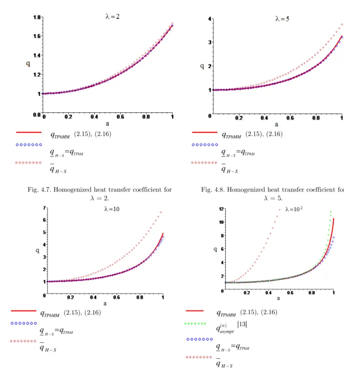
1) In Figures 3.1 to 3.10 graphs of the homogenized heat transfer coefficient yielded by the TPhMM for various values of the heat transfer inclusions are reported:
~ 1 0.8; 1.25 , see Figures 4.5 and 4.6.
1 2; 5 , see Figures 4.7 and 4.8.
1 10; 102 , see Figures 4.9 and 4.10.
In order to compare the obtained results, the Hashin-Shtrickman (H-S) boundaries are also re-ported [6, 7, 18] which are defined through the following relations
2 2 2 2
2 2 2 2
2 2 2 2
2 2 2 2
1 1 2
4 4 4 4
1 1 2
4 4 4 4
H S
H S
a a a a
b b b b
q q q
a a a a
b b b b
for 1 ; (4.1)
2 2
2 2
2 2
2 2
2 2 2 2
2 2 2 2
1 1
2
4 4
4 4
2 1 1
4 4 4 4
H S
H S
a a
a a
b b
b b q q q
a a a a
b b b b
for 0 1. (4.2)
(4.2)
It is worth noting that the solution obtained via the TPhM identically coincides with the lower boundary of the H-S estimation for 1 and regarding the upper boundary for 0 1.
TPhMM
q (2.15) and (2.16) 0
аsympt
q [9,13]
ТPhM S
H q
q
H S
q
ТPhММ
q (2.15) and (2.16)
ТPhM S
H q
q
H S
q
Fig. 4.1. Homogenized heat transfer coefficient for 10 .2
Fig. 4.2. Homogenized heat transfer coefficient for
1
TPhMM
q (2.15), (2.16)
ТPhM S
H q
q
H S
q
TPhMM
q (2.15), (2.16)
ТPhM S
H q
q
H S
q
Fig. 4.3. Homogenized heat transfer coefficient for
0.2.
Fig. 4.4. Homogenized heat transfer coefficient for
0.5.
TPhMM
q (2.15), (2.16)
ТPhM S
H q
q
H S
q
TPhMM
q (2.15), (2.16)
ТPhM S
H q
q
H S
q
Fig. 4.5. Homogenized heat transfer coefficient for
0.8.
Fig. 4.6. Homogenized heat transfer coefficient for
2) Graphs related to the cases of geometrically large inclusions a 1 , and either large
or small 0 heat homogenized transfer coefficients and that computed by the TPhMM as well as those obtained in [9,13] are shown in Figures 4.11 - 4.14. The asymptotic solution obtained in [13] is as follows
TPhMM
q (2.15), (2.16)
ТPhM S
H q
q
H S
q
TPhMM
q (2.15), (2.16)
ТPhM S
H q
q
H S
q
Fig. 4.7. Homogenized heat transfer coefficient for
2.
Fig. 4.8. Homogenized heat transfer coefficient for
5.
TPhMM
q (2.15), (2.16)
ТPhM S
H q
q
H S
q
TPhMM
q (2.15), (2.16)
аsympt
q [13]
ТPhM S
H q
q
H S
q
Fig. 4.9. Homogenized heat transfer coefficient for
10.
2 1 1
sympt
q
a
а for , a 1, (4.3)
whereas that obtained in [9, 13] has the following form
2 0
2 1
1 1
sympt
a q
a
а for 0, a 1. (4.4)
While constructing the dependencies shown in Figures 4.1 to 4.10, a solution to the transcenden-tal Eqs. (2.15) and (2.16) has been found numerically, whereas dependencies in the vicinity of the limiting values of parameters ,a 1 and 0,a 1 (Figures 4.11 to 4.14) have been
constructed with the help of asymptotic formulas (2.2) and (2.4), respectively.
ТPhММ
q (3.2)
аsympt
q [13]
ТPhM S
H q
q
ТPhММ
q (3.2)
аsympt
q [13]
ТPhM S
H q
q
Fig. 4.11. Homogenized heat transfer coefficient
for 5
10 , a 1.
Fig. 4.12. Homogenized heat transfer coefficient for , 1.
3) For small size of the inclusions a 1 and various values of heat transfer the equivalent heat transfer parameter obtained through TPhMM in comparison to the Schwarz alternating meth-od [1] are given in Figures 4.15 to 4.22.
ТPhММ
q (3.4)
0
аsympt
q [9,13]
ТPhM S
H q
q
ТPhММ
q (3.4)
0
аsympt
q [9,13]
ТPhM S
H q
q
Fig. 4.13. Homogenized heat transfer coefficient for 10 5, a 1.
Fig. 4.14. Homogenized heat transfer coefficient for 0, 1.
a
ТPhММ
q (2.15), (2.16)
Schwarz method [1]
ТPhM S
H q
q
ТPhММ
q (2.15), (2.16)
Schwarz method [1]
ТPhM S
H q
q
H S
q
Fig. 4.15. Homogenized heat transfer coefficient for
0, a 1.
Fig. 4.16. Homogenized heat transfer coefficient for
2
ТPhММ
q (2.15), (2.16)
Schwarz method [1]
ТPhM S
H q
q
H S
q
ТPhММ
q (2.15), (2.16)
Schwarz method [1]
ТPhM S
H q
q
H S
q
Fig. 4.17. Homogenized heat transfer coefficient for
1
10 , a 1.
Fig. 4.18. Homogenized heat transfer coefficient for
0.5, a 1.
ТPhММ
q (2.15), (2.16)
Schwarz method [1]
ТPhM S
H q
q
H S
q
ТPhММ
q (2.15), (2.16)
Schwarz method [1]
ТPhM S
H q
q
H S
q
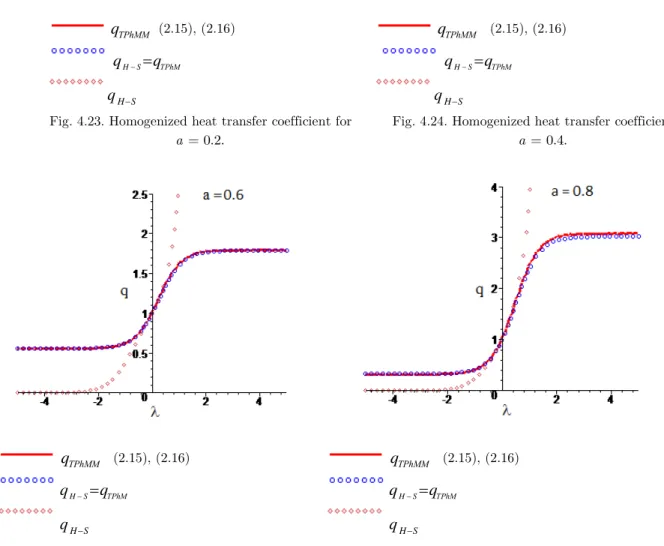
4) Figures 4.23 to 4.26 give the dependencies of the homogenized heat transfer coefficient obtained through the TPhMM for various values of the inclusions size a. Namely, we have small inclusions:
0.2
a (Fig. 4.15), inclusions of average size: a 0.4; a 0.6 (Figs. 4.16 and 4.17), large
inclu-sions: a 0.8 (Fig. 4.18).
Upper qH S and lower qH S Hashin-Shtrickman boundaries are marked, and the TPhM
solu-tion coinciding with qH S for 1 and with qH S for 0 1 is given. ТPhММ
q (2.15), (2.16)
Schwarz method [1]
ТPhM S
H q
q
H S
q
ТPhММ
q (2.15), (2.16)
Schwarz method [1]
ТPhM S
H q
q
H S
q
Fig. 4.21. Homogenized heat transfer coefficient for
2
10 , a 1.
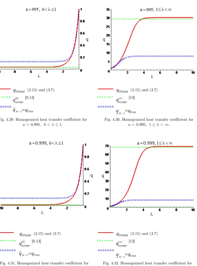
5) Graphs shown in Figures 4.27 to 4.32 illustrate the behaviour of equivalent heat transfer coeffi-cient versus conductivity of the inclusions of large size a 1. While constructing the graphs
asymptotic formulas (2.15) and (3.7) have been used. In addition, the dependencies qаsympt and
0
sympt
qа , constructed on the basis of (4.3) and (4.4), are added [9,13].
ТPhММ
q (2.15), (2.16)
ТPhM S
H q
q
H S
q
ТPhММ
q (2.15), (2.16)
ТPhM S
H q
q
H S
q
Fig. 4.23. Homogenized heat transfer coefficient for 0.2.
a
Fig. 4.24. Homogenized heat transfer coefficient for 0.4.
a
ТPhММ
q (2.15), (2.16)
ТPhM S
H q
q
H S
q
ТPhММ
q (2.15), (2.16)
ТPhM S
H q
q
H S
q
Fig. 4.25. Homogenized heat transfer coefficient for 0.6.
a
Fig. 4.26. Homogenized heat transfer coefficient for a 0.8.
ТPhММ
q (2.15) and (3.7)
0
аsympt
q [9,13]
ТPhM S
H q
q
ТPhММ
q (2.15) and (3.7)
аsympt
q [13]
ТPhM S
H q
q
Fig. 4.27. Homogenized heat transfer coefficient for
0.99, 0 1.
a
Fig. 4.28. Homogenized heat transfer coefficient for
0.99, 1 .
ТPhММ
q (2.15) and (3.7)
0
аsympt
q [9,13]
ТPhM S
H q
q
ТPhММ
q (2.15) and (3.7)
аsympt q [13]
ТPhM S
H q
q
Fig. 4.29. Homogenized heat transfer coefficient for
0.995, 0 1.
a
Fig. 4.30. Homogenized heat transfer coefficient for
0.995, 1 .
a
ТPhММ
q (2.15) and (3.7)
0
аsympt q [9,13]
ТPhM S
H q
q
ТPhММ
q (2.15) and (3.7)
аsympt q [13]
ТPhM S
H q
q
Fig. 4.31. Homogenized heat transfer coefficient for
0.999, 0 1.
a
Fig. 4.32. Homogenized heat transfer coefficient for
0.999, 1 .
6) For the case of a composite structure with absolute heat transfer and of large size
1
a a comparison of the results regarding the effective computations of heat transfer coefficient
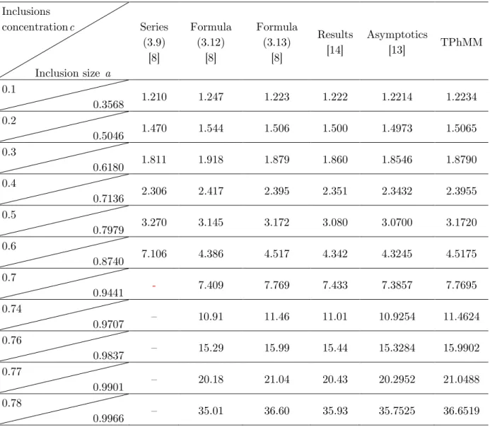
found via the TPhMM with those reported by other authors are given in Tables 4.1 and 4.2.
Table 4.1. Numerical results of the estimation of heat transfer coefficient (absolutely conductive inclusions).
Table 4.2. Numerical and analytical results of the estimation of heat transfer coefficient (absolutely conductive inclusions).
Inclusions concentrationc
Inclusion size a
Series (3.9)
[8]
Formula (3.12)
[8]
Formula (3.13)
[8]
Results [14]
Asymptotics
[13] TPhMM
0.1
0.3568 1.210 1.247 1.223 1.222 1.2214 1.2234
0.2
0.5046 1.470 1.544 1.506 1.500 1.4973 1.5065
0.3
0.6180 1.811 1.918 1.879 1.860 1.8546 1.8790
0.4
0.7136 2.306 2.417 2.395 2.351 2.3432 2.3955
0.5
0.7979 3.270 3.145 3.172 3.080 3.0700 3.1720
0.6
0.8740 7.106 4.386 4.517 4.342 4.3245 4.5175
0.7
0.9441 - 7.409 7.769 7.433 7.3857 7.7695
0.74
0.9707 – 10.91 11.46 11.01 10.9254 11.4624
0.76
0.9837 – 15.29 15.99 15.44 15.3284 15.9902
0.77
0.9901 – 20.18 21.04 20.43 20.2952 21.0488
0.78
0.9966 – 35.01 36.60 35.93 35.7525 36.6519
Parameter 1 1 a2
Inclusion size a
Numerical com-putation [13]
Asymptotics
[13] TPhMM
7) Table 4.3 gives computational results of the homogenized heat transfer coefficient obtained using the TPhMM and their comparison with the analytical solution given in reference [13] for the case of the inclusion size 0 a 1 and large heat conductivity 0 .
Table 4.3. Computational results of the estimation of effective heat transfer coefficient (large size and large conduc-tivity of inclusions).
0.9949874370 20
0.9987492180 60.8976 60.6903 61.6814
30
0.9994442899 92.3575 92.1062 93.1460
40
0.9996874512 123.7734 123.5221 124.5868
50
0.9997999801 155.1894 154.9380 156.0179
100
0.9999499986 312.6460 312.0177 313.1276
1000
0.9999995001 3142.5927 3142.5927 3140.9037
Inclusion conductivity 102 Inclusion conductivity 5 102
Inclusion size a
Asymptotic
solution [13] TPhMM
Inclusion size a
Asymptotic
solution [13] TPhMM
0.9 4.9108 5.0044 0.9 5.0347 5.2456
0.91 5.2473 5.3449 0.91 5.3980 5.6282
0.92 5.6413 5.7411 0.92 5.8277 6.0792
0.93 6.1112 6.2097 0.93 6.3467 6.6213
0.94 6.6841 6.7753 0.94 6.9901 7.2893
0.95 7.4037 7.4765 0.95 7.8164 8.1407
0.96 8.3438 8.3770 0.96 8.9315 9.2776
0.97 9.6432 9.5934 0.97 10.5536 10.9067
0.98 11.5936 11.3680 0.98 13.2351 13.5334
0.99 14.8171 14.3260 0.99 19.0663 18.9367
0.991 15.2200 14.7431 0.991 20.1058 19.8518
0.992 15.6149 15.1940 0.992 21.3187 20.8999
0.993 15.9721 15.6836 0.993 22.7595 22.1169
0.994 16.2297 16.2179 0.994 24.5101 23.5539
0.995 16.2513 16.8041 0.995 26.7012 25.2868
Heat transfer of inclusions
3 10
Heat transfer of inclusions
5 10
8) In reference [1] for small inclusion size a 1, the formula for equivalent heat transfer coeffi-cient obtained using the Schwarz method of successive approximations is reported. Table 4.4 gives the computational results of homogenized heat transfer coefficient using ThPM [16] as well as the Schwarz method [1] and the TPhMM for the case of various heat transfer and small values of the inclusion size a.
Table 4.4. Computational results of the estimation of effective heat transfer coefficient (small size of inclusions).
size a solution [13] size a solution [13]
0.9 5.0502 5.2776 0.9 5.0656 5.3099
0.91 5.4168 5.6661 0.91 5.4355 5.7043
0.92 5.8510 6.1249 0.92 5.8741 6.1709
0.93 6.3761 6.6774 0.93 6.4053 6.7342
0.94 7.0283 7.3605 0.94 7.0662 7.4325
0.95 7.8680 8.2343 0.95 7.9190 8.3297
0.96 9.0049 9.4080 0.96 9.0776 9.5418
0.97 10.6674 11.1050 0.97 10.7801 11.3109
0.98 13.4403 13.8868 0.98 13.6435 14.2620
0.99 19.5974 19.8425 0.99 20.1233 20.8685
0.991 20.7166 20.8903 0.991 21.3212 22.0828
0.992 22.0317 22.1070 0.992 22.7376 23.5164
0.993 23.6079 23.5437 0.993 24.4478 25.2448
0.994 25.5452 25.2763 0.994 26.5699 27.3860
0.995 28.0074 27.4232 0.995 29.3006 30.1366
Inclusion conductivity 0 Inclusion conductivity 10 2
Inclusion size a
TPhM [16]
Schwarz
method [1] TPhMM
Inclusion size a
TPhM [16]
Schwarz
method [1] TPhMM
0.05 0.9961 0.9961 0.9961 0.05 0.9962 0.9962 0.9962
0.1 0.9844 0.9844 0.9844 0.1 0.9847 0.9847 0.9847
0.15 0.9653 0.9650 0.9653 0.15 0.9659 0.9657 0.9659
0.2 0.9391 0.9382 0.9391 0.2 0.9403 0.9394 0.9402
0.25 0.9064 0.9044 0.9064 0.25 0.9082 0.9063 0.9082
0.3 0.8680 0.8639 0.8679 0.3 0.8704 0.8666 0.8704
Inclusion conductivity 10 1 Inclusion conductivity 0.5
Inclusion size a
TPhM [16]
Schwarz
method [1] TPhMM
Inclusion size a
TPhM [16]
Schwarz
method [1] TPhMM
0.05 0.9968 0.9968 0.9968 0.05 0.9987 0.9987 0.9987
0.1 0.9872 0.9872 0.9872 0.1 0.9948 0.9948 0.9948
Table 4.5 gives the mean absolute discrepancy of the computation of effective heat transfer coef-ficient using the TPhMM versus known results obtained by other authors.
Table 4.5. Mean value of the absolute discrepancy of the estimation of heat transfer coefficient using the TPhMM and results obtained by other authors in %
0.25 0.9228 0.9218 0.9228 0.25 0.9678 0.9681 0.9678
0.3 0.8907 0.8887 0.8906 0.3 0.9540 0.9546 0.9540
Inclusion conductivity 2 Inclusion conductivity 10
Inclusion size a
TPhM [16]
Schwarz
method [1] TPhMM
Inclusion size a
TPhM [16]
Schwarz
method [1] TPhMM
0.05 1.0013 1.0013 1.0013 0.05 1.0032 1.0032 1.0032
0.1 1.0052 1.0052 1.0052 0.1 1.0129 1.0130 1.0129
0.15 1.0119 1.0118 1.0119 0.15 1.0293 1.0295 1.0293
0.2 1.0212 1.0210 1.0212 0.2 1.0528 1.0532 1.0528
0.25 1.0333 1.0329 1.0333 0.25 1.0839 1.0849 1.0837
0.3 1.0483 1.0475 1.0483 0.3 1.1228 1.1253 1.1228
Inclusion conductivity 102 Inclusion conductivity
Inclusion size a
TPhM [16]
Schwarz method
[1]
TPhMM Inclusion
size a
TPhM [16]
Schwarz
method [1] TPhMM
0.05 1.0039 1.0038 1.0039 0.05 1.0039 1.0039 1.0039
0.1 1.0155 1.0153 1.0156 0.1 1.0158 1.0159 1.0158
0.15 1.0353 1.0343 1.0355 0.15 1.0360 1.0363 1.0360
0.2 1.0635 1.0606 1.0645 0.2 1.0649 1.0659 1.0649
0.25 1.1011 1.0937 1.1034 0.25 1.1032 1.1057 1.1033
0.3 1.1489 1.1334 1.1539 0.3 1.1521 1.1575 1.1522
1. Inclusions: Mean size : 0.3568 a 0.8740
Absolute conductivity: Formula (3.9)
[8]
Formula (3.12) [8]
Formula (3.13) [8]
Results [14]
Asymptotics [13]
3.2790 2.3457 0.0119 2.4839 2.8573
2. Inclusions: Large size : 0.9441 a 0.9966 Absolute conductivity:
Formula (3.12) [8]
Formula (3.13) [8]
Results [14]
Asymptotics [13]
4.6594 0.0515 3.1776 3.8654
5 CONCLUSIONS
One may conclude from the data reported in Table 4.1 and from the paper text body that our re-sults constructed through the proposed improved TPhM allow us to improve the rere-sults obtained via the classical TPhM approach regarding the estimation of effective heat transfer parameter of the
Numerical computation [13]
Asymptotics [13]
0.5899 0.7884
4. Inclusions: Large size : 0.9 a 995 Large conductivity: 102 105
Asymptotics [13]
3.1354
5. Inclusions: Small size : 0 a 0,3
Non-conductivity: 0
PhM [16] Schwarz method [1]
0.0016 0.1159
6. Inclusions: Small size : 0 a 0.3
Small conductivity: 10 2 10 1
PhМ [16] Schwarz method [1]
0.0016 0.0814
7. Inclusions: Small size : 0 a 0.3
Matrix magnitude conductivity: 0.5 2
PhМ [16] Schwarz method [1]
0.0000 0.0178
8. Inclusions: Small size : 0 a 0,3
Large conductivity: 10 100
PhМ [16] Schwarz method [1]
0.0561 0.2585
9. Inclusions: Small size : 0 a 0,3
Absolute conductivity:
PhM [16] Schwarz method [1]
composite structure with periodically located cylindrical inclusions of circular cross-sections on the square net.
Finally, let us emphasise that the TPhMM is practically validated and gives reliable results in the whole area of both composite parameters variation, i.e. with respect to:
(i) geometric parameter regarding the size of inclusions a: 0 a 1;
(ii)physical parameter regarding the inclusion conductivity : 0 , including the limiting
cases:a 0, a 1 and 0, .
References
1. I.V. Andrianov, G.A. Starushenko, Asymptotic methods in the theory of perforated membranes of nonhomoge-neous structure, Eng. Trans. 43 (1995) 5-18.
2. I.V. Andrianov, G.A. Starushenko, V.V. Danishevs’kyy, S. Tokarzewski, Homogenization procedure and Padé approximations in the theory of composite materials with parallelepiped inclusions, Int. J. Heat Mass Transfer 41(1) (1998) 175-181.
3. I.V. Andrianov, G.A. Starushenko, V.V. Danishevs’kyy, S. Tokarzewski, Homogenization procedure and Padé approximants for effective heat conductivity of composite materials with cylindrical inclusions having square cross-section, Proc. R. Soc. A 455 (1999) 3401-3413.
4. R.M. Christensen, Mechanics of Composite Materials, Dover Publications, Mineola, New York, 2005.
5. R.M. Christensen, K.H. Lo, Solutions for effective shear properties in three phase sphere and cylinder models, J. Mech. Phys. Solids 27 (1979) 315-330.
6. Z. Hashin, S. Shtrikman, A variational approach to the theory of the effective magnetic permeability of multi-phase materials, J. Math. Phys. 33 (1962) 3125-3131.
7. Z. Hashin, S. Shtrikman, A variational approach to the theory of the elastic behaviour of multiphase materials, J. Mech. Phys. Solids 11 (1963) 127-140.
8. A.L. Kalamkarov, I.V. Andrianov, V.V. Danishevs’kyy, Asymptotic homogenization of composite materials and structures, Appl. Mech. Rev. 62(3) (2009) 030802-1 – 030802-20.
9. J.B. Keller, A theorem on the conductivity of a composite medium, J. Math. Phys. 5 (1964) 548-549. 10. E.H. Kerner, The electrical conductivity of composite media, Proc. Physics Soc. B 69(8), (1956) 802-807. 11. E.H. Kerner, The elastic and thermoelastic properties of composite media, Proc. Physics Soc. B 69(8) (1956)
808-813.
12. J.-L. Lions, On some homogenisation problem, ZAMM 62(5) (1982) 251-262.
13. R. . McPhedran, L. Poladian, G.W. Milton, Asymptotic studies of closely spaced, highly conducting cylinders, Proc. R. Soc. A 415 (1988) 185-196.
14. W.T. Perrins, D.R. McKenzie, R.C. McPhedran, Transport properties of regular arrays of cylinders,Proc. R. Soc. A 369 (1979) 207-225.
15. G.A. Starushenko, B.E. Rogoza, Review and analysis of three-phase model in mechanics of composites, Part I, Systems Technol., Dnepropetrovsk 5(52) (2007) 3-10 (in Russian).
16. G.A. Starushenko, B.E. Rogoza, Review and analysis of three-phase model in mechanics of composites, Part II, Systems Technol., Dnepropetrovsk 1(54) (2008) 3-12 (in Russian).
17. C. Van der Poel, On the rheology of concentrated dispersions, Rheol. Acta 1(2-3) (1958) 198-205.