http://dx.doi.org/10.20852/ntmsci.2016115854
Euler-Lagrange equations for holomorphic structures on
twistorial generalized K ¨ahler manifolds
Zeki Kasap
Elementary Mathematics Education Department, Pamukkale University, Denizli, Turkey Received: 23 November 2015, Revised: 7 December 2015, Accepted: 22 December 2015 Published online: 10 February 2016.
Abstract: The paper aims to introduce some partial differential equations on Twistorial generalized K¨ahler manifolds, with an emphasis on Euler-Lagrange equations. Twistor spaces are certain complex 3-manifolds which are associated with special conformal Riemannian geometries on 4-manifolds. Also, classical mechanic is one of the major subfields for mechanics system. A mechanical system has a state determined by a collection of real numbers, or more generally by a set of points in an appropriate state space. Euler-Lagrange equations are an efficient use of classical mechanics to solve problems using mathematical modeling. In this study, showing motion modeling partial differential equations have been obtained for movement of objects in space and solutions of these equations have been generated by using the Maple software. Additionally, of the implicit solution of the equations to be drawn the graph.
Keywords: Twistor, K¨ahlerian manifold, mechanical system, dynamic equation, almost complex, lagrangian formalism.
1 Introduction
Dynamic systems are a recent theoretical and applied approach to the study of development. In its contemporary formulation, the theory grows directly from advances in understanding complex and nonlinear systems in mathematical physics and differential geometry. A dynamical system is a smooth action of the real or the integers on another object that it named usually a manifold. At any given time of a dynamical system has a state given by a set of a vector that can be represented by a point in an appropriate state space. Also, dynamical systems theory attempts to encompass all the possible factors that may be in operation at any given developmental moment; it considers development from many levels and time scales. Classical mechanics has provided effective solution methods using Euler-Lagrange equations for dynamic systems. Euler-Lagrange equation is one of these methods and it is a model that shows the movement over time of dynamic systems of quantum mechanics. Twisted geometries are discrete geometries that plays a role in loop quantum gravity and spin foam models, where they appear in the semiclassical limit of spin networks and a spin network is a type of diagram which can be used to represent states and interactions between particles and fields in quantum mechanics. Twistor theory was created by Penrose [1]. Penrose created the twistor theory to solve problems in mathematical physics [2]. Freidela and Speziale showed that the phase space of loop quantum gravity on a fixed graph can be parametrized in terms of twisted geometries, quantities describing the intrinsic and extrinsic discrete geometry [3]. Speziale introduced
that loop quantum gravity and twisted geometries [4]. Santa-Cruz presented the hyperk¨ahler geometry of complex
adjoint orbits from the point of view of twistor theory [5]. Albuquerque used twistor theory to describe virtually new
constructions of Hermitian and quaternionic K¨ahler structures on tangent bundles [6]. Davidov and Mushkarov
natural class of twistorial maps gives a pattern for apparently different geometric maps, such as, (1,1)-geodesic immersions from(1,2)-symplectic almost Hermitian manifolds and pseudo horizontally conformal submersions with totally geodesic fibres for which the associated almost CR-structure is integrable [9]. Ianus et al introduced a natural
notion of quaternionic map between almost quaternionic manifolds [10]. Dunajski examined an elementary and
self–contained review of twistor theory as a geometric tool for solving non-linear differential equations.[11].
Marchiafava obtained that an alternative proof of a characterization of twistorial maps between quaternionic projective
spaces [12]. Kasap found Weyl-Euler-Lagrange equations of motion on flat manifold [13]. Tekkoyun revealed
Euler-Lagrange and Hamiltonian equations onR2n
n which is a model of para-K¨ahlerian manifolds of constant J-sectional
curvature [14]. Cecotti et al defined twistorial topological strings by considering tt∗ geometry of the 4d N=2
supersymmetry theories on the Nekrasov-Shatashvili12Ω background [15].
2 Preliminaries
Definition 1.AHermitian formon a vector space V over the complex field Cis a function f :V×V →Csuch that for all u,v,w in V and all a,b inR, 1. f(au+bv,w) =a f(u,w) +b f(v,w).2. f(u,v) = f¯(v,u).Here, the bar indicates
the complex conjugate. It follows that f(u,av+bw) =a f¯ (u,v) +b f¯ (u,w), which can be expressed by saying that f is antilinear on the second coordinate.
Definition 2.Let−→X = (xi),Y= (yi)∈R3be any two vectors. As follows
<, >:R3×R3→R1, <−→X,Y>L=−x1y1+x2y2+x3y3 (1)
in the form of a function. This function are bilinear and symmetric. This the inner product function<X,Y >Lalong with
R3is called Minkowski space or the Lorenz space and it is been shownR3 1.
Theorem 1.Let X∈R3
1be any one vector.
(1) If<−→X,−→X >L>0or
− →
X =−→0,−→X is spacelike,
(2) If<−→X,−→X >L<0,
− →
X is timelike,
(3) If<−→X,−→X >L<0,−→X is lightlike (isotropic, null).
Definition 3.Minkowski space is a four-dimensional space possessing a Minkowski metric a metric tensor having the form
dτ2=−(dx0)2+ (dx1)2+ (dx2)2+ (dx3)2. (2)
In equation (2) above, the metric signature(1,3)is assumed; under this assumption, Minkowski space is typically written
R(1,3). One may also express equation (2) with respect to the metric signature(3,1)by reversing the order of the positive
and negative squared terms therein, in which case Minkowski space is denotedR(1,3).
Definition 4.Suppose thatξis a vector field: that is, a vector-valued function with Cartesian coordinates(ξ1, ...,ξn); and
x(t)a parametric curve with Cartesian coordinates(x1(t), ...,xn(t)). Thenx(t)isan integral curveofξ if it is a solution
of the following autonomous system of ordinary differential equations:dx1
dt =ξ1(x1, ...,xn), ..., dxn
dt =ξn(x1, ...,xn).Such a
system may be written as a single vector equation
ξ(x(t)) =x′(t) = ∂
2.1 J-Holomorphic curve
Definition 5.Let be V a vector space over R. Let M be a differentiable manifold of dimension2n, and suppose J is a
differentiable vector bundle isomorphism Jx:TxM→TxM.
(1) A (almost) complex structureon M for J2d=−Id.
(2) A (almost) paracomplex structureon M for J2d=Id.
(3) Atangent (exact) structureon M for J2d=0.
Where J2=J◦J, and I is the identity (unit) operator on V by the map J:V →V and V =Rn⊕Rn.
Definition 6.A tangent structure J on M assigns to each p∈M a linear map Jp:TpM→TpM that is smooth in p and
satisfies J2pd=0for all p. The pair(M,J)is calleda tangent manifold.
Theorem 2.Any complex manifold M is also an almost complex manifold.
Lemma 1.Let M be a smooth manifold. If M admits a complex structure A, then M admits an almost complex structure J. Let dimCM=m and(z,U)be any holomorphic chart inducing a coordinate frame∂x1,∂y1, ...,∂xm,∂ym. Then J is given
locally as
Jp(∂xip) =∂yip , Jp(∂yip) =−∂xip, (4)
where1≤i≤m and p∈U [16].
J-holomorphic curve is a smooth map from a Riemann surface into an almost complex manifold that satisfies the Cauchy–
Riemann equation.
Definition 7. Let (M,ω)be a symplectic manifold of dimension 2n, and let J ∈J(M,ω) be anω-compatible almost complex structure. Let gJ(·,·)≡ω(·,J·)be the corresponding Hermitian metric on M.
Definition 8.Let (∑, j)be a Riemann surface with complex structurej. A smooth map u:∑→M is called a(J,j) -holomorphic map (or simply a J--holomorphic map) if du◦j=J◦du, or equivalently,
¯ ∂J(u) =
1
2(du+J◦du◦j) =0. (5)
The equation∂¯J(u) =0is a first order, non-linear equation of Cauchy-Riemann type.
3 Twistor theory
Twisted geometries are discrete geometries that plays a role in loop quantum gravity, where they appear in the semiclassical limit of spin networks and it maps the geometric objects of conventional 3+1 space-time (Minkowski space) into geometric objects in a 4-dimensional space endowed with a Hermitian form of signature (2,2). This space is calledtwistor space, and its complex valued coordinates are calledtwistors.
Definition 9. (Twistor space) If (M,g)is an oriented Riemannian2n-manifold then:Z is the bundle of g-orthogonal positive complex structures on the tangent spaces of M andτ:Z→M is the bundle projection. The fibre F=τ−1(x)is the space of J∈End(TxM)such that (a) J2=−id,(b) g(Jv,Jw) =g(v,w)for all v,w∈TxM.
Theorem 3.(Eells-Salamon 1985, Twistor correspondence) Let M be a Riemannian 2n-manifold. There is an almost complex n(n+1)-manifold(Z,J),the twistor spaceof M,and a mapτ:Z→M such that (a) J-holomorphic curves inZ
3.1 Generalized K¨ahler structures
Definition 10.Let(M,J,g)be a2n-dimensional almost complex manifold and g is a metric, i.e. J is analmost complex structuresuch that J2X=−X,g(JX,JY) =−g(X,Y),for all vector fields X , Y on M and g is a metric.
Definition 11.Let M be a complex manifold with complex structure J and compatible Riemannian metric g=< ., . >as in
<JX,JY>=<X,Y>. The alternating2-formω(X,Y):=g(JX,Y)is called the associatedK¨ahler form. We can retrieve g fromω, g(X,Y) =ω(X,JY).We can say that g is a K¨ahler metric and that M is aK¨ahler manifoldifω is closed and
(M,g)is displayed in the form.
Definition 12.Let M be a complex manifold. A Riemannian metric on M is called Hermitian if it is compatible with the complex structure J of M,<JX,JY >=<X,Y >. Then the associated differential two-formω defined byω(X,Y) =<
JX,Y >is called the K¨ahler form. It turns out thatω is closed if and only if J is parallel. Then M is called aK¨ahler manifoldand the metric on M a K¨ahler metric. K¨ahler manifolds are modelled on complex Euclidean space [17].
Definition 13.Let V be a2n-dimensional real vector space and let{∂∂x
i+ ∂
∂yi}, i=1, ...,4n, be an orthonormal basis of the space V⊗V∗endowed with the neutral metric (6). Then ∂∂x
1,..., ∂
∂x2n is a basis of V and ∂ ∂y1,...,
∂
∂y2n is a basis of V
∗.
Definition 14.Let V⊗V∗be a n-dimensional real vector space and g a metric of signature(p,q)on it, p+q=n.We shall say that an orthogonal basis{∂∂x
1, ..., ∂
∂xn}of V⊗V
∗is orthonormal if
∂ ∂x1
2 =···= ∂ ∂xp+q
2
=−1. If n=2m is an even number and p=q=m, the metric g is usually called neutral. Recall that a complex structure J on V⊗V∗is
called compatible with the metric g, if the endomorphism J is g-skew-symmetric. Suppose that p=2k and q=2l, and
let J be a compatible complex structure on V⊗V∗. Then it is easy to see by induction that there is an orthonormal basis
{∂∂x
1, ..., ∂
∂xn}of V⊗V
∗such that J ∂ ∂x2i−1 =
∂
∂x2i, i=1, ...,k+l.
Definition 15.Let V be a2n-dimensional real vector space and V∗its dual space. Then the vector space V⊕V∗admitsa natural neutral metricdefined by
⟨X+ξ,Y+η⟩=1
2(ξ(Y) +η(X)), X,Y ∈V andξ,η∈V
∗. (6)
LetV be a 2-dimensional real vector space and let{Qi=∂∂x
i + ∂ ∂yi
}
,1≤i≤4, be an orthonormal basis of the space
V⊕V∗endowed with its natural neutral metric (6). Then
∂ ∂x3
=a11 ∂ ∂x1
+a12 ∂ ∂x2
, ∂
∂x4
=a21 ∂ ∂x1
+a22 ∂ ∂x2
(7)
whereA= [ai j] is an orthogonal matrix. IfdetA=1, the basis {Qi}yields the canonical orientation ofV⊕V∗ and if
detA=−1 it yields the opposite one (proof see [7]).
Theorem 4.Let V be a 2-dimensional real vector space. Take a basis{∂∂x
1, ∂
∂x2}of V and let{ ∂ ∂y1,
∂ ∂y2}of V
∗be its dual
basis. Then{Q1=∂∂x 1+
∂ ∂y1,Q2=
∂
∂x2+
∂ ∂y2,Q3=
∂
∂x3−
∂ ∂y3,Q4=
∂
∂x4−
∂
∂y4 }is an orthonormal basis of V⊗V
∗with
respect to the natural neutral metric (2) and is positively oriented with respect to the canonical orientation of V⊗V∗.
Set εk =∥Qk∥2, k=1, ...,4, and define skew-symmetric endomorphisms of V ⊗V∗ setting Si jQk=εk(δikQj−δikQ),
1≤i,j,k≤4. Then the endomorphisms
I1=S12−S34,J1=S12+S34,
I2=S13−S24,J2=S13+S24,
I3=S14+S23,J3=S14−S23,
constitute a basis of the space of skew-symmetric endomorphisms of V⊗V∗subject to the following relations:
I12=I22=Id,I32=0,
J12=J22=Id,J32=0
IrIs=−IsIr, JrJs=−JsJr, 16r̸=s63
IrJs=JsIr, 16r,s63.
(9)
LetΨ be a complex structure onV⊗V∗ compatible with the metric and let us setΨ =∑3r=1(xrIr+yrJr). Then we
haveΨ2=Idif and only if eitherI=∑
rxrIr withx21+x22=1 andy1=y2=y3=0,J=∑sysJs withy21+y22=1 and x1=x2=x3=0.It follows that
I∂∂x 1 =x1
∂
∂x1+ (x2+1) ∂ ∂x2, J
∂ ∂x1 =y1
∂
∂x1+ (y2−1) ∂ ∂y2, I∂∂x
2 = (x2−1) ∂ ∂x1 −x1
∂ ∂x2, J
∂ ∂x2 =y1
∂
∂x2+ (y2−1) ∂ ∂y1, I∂∂
y1 =−x1 ∂
∂y1 −(x2−1) ∂ ∂y2, J
∂
∂y1 = (y2+1) ∂ ∂x2−y1
∂ ∂y1 I∂∂y
2 =−(x2+1) ∂ ∂y1+x1
∂ ∂y2,J
∂
∂y2 = (y2+1) ∂ ∂x1−y1
∂ ∂y2.
(10)
This shows that the restriction ofItoV is a complex structure onV inducing the generalized complex structureI. In contrast, the generalized complex structureJis not induced by a complex structure or a symplectic form onV.
Proof.Let us setΨ=∑3r=1(xrIr+yrJr).Let’s we have accountΨ2using Definition 5 :
Ψ2=∑3
r=1(xrIr+yrJr)2
=x21I12+x22I22+x23I32+y21J12+J22y22+J32y23+2∑r3,s=1(xrysIrJs). =x21+x22+y21+y22+2∑3r,s=1(xrysIrJs).
(11)
We see thatx21+x22+y21+y22=1,xrys=0,r,s=1,2,3.ThereforeΨ2=Idif and only if eitherx12+x22=1 fory1=y2= y3=0 andy21+y22=1 forx1=x2=x3=0 [7].
Theorem 5.Ifαandβ are 1-forms, thenα∧βis a 2-forms.
Definition 16.In three dimensions, the vector from the origin to the point with Cartesian coordinates(x,y,z)can be written as [18]:
r=xi+yj+zk=x
(∂ ∂x ) +y (∂ ∂y ) +z (∂ ∂z ) . (12)
Proposition 1.Let−→X ,Y∈R3
1be any two vector that are.
− →
X = (x,y+1,0),Y= (y−1,−x,0).Let this curve expressed as vectors:
r1=x (∂
∂x
)
+ (y+1) (∂
∂y
)
, r2= (y−1) (∂ ∂x ) −x (∂ ∂y ) . (13)
Example 1. Let us consider the structure (10) using the holomorphic property at (13). We can define the following
holomorphic structureswith:
(1)J∂∂x=x∂∂x+ (y+1)∂∂y,
(2)J∂∂y= (y−1)∂∂x−x∂∂y. (14)
Now, we denote the structure (14) of the holomorphic property:
(1)J2∂
∂x=x
(
x∂∂
x+ (y+1)
∂ ∂y
)
+ (y+1)((y−1)∂∂x−x∂∂
y
)
= (x2+y2−1)∂ ∂x. (2)J2∂
∂y= (y−1)
(
x∂∂x+ (y+1)∂∂y)−x((y−1)∂∂x−x∂∂y)= (x2+y2−1)∂ ∂y.
As shown above, the structures (15) are tangent (Defintion5) andx2+y2=1 forJ2=0.This is a cone and the graph is as follows:
4 (Euler)-Lagrange dynamics equations
Lemma 2.The closed2-form on a vector field and1−form reduction function on the phase space defined of a mechanical system is equal to the differential of the energy function1-form of the Lagrangian and the Hamiltonian mechanical systems
[19,20].
Definition 17.Let M be an n-dimensional manifold and T M its tangent bundle with canonical projectionτM:T M→M.
T M is called the phase space of velocities of the base manifold M. Let L:T M→R be a differentiable function on T M
called theLagrangian function. Here, L=T−V such that T is the kinetic energy and V is the potential energy of a
mechanical system. In the problem of a mass on the end of a spring, T=mx˙2/2and V=kx2/2.
Definition 18.We consider the closed2-form and base space(J)on T M given byΦL=−d(dJL) =−d(J(d)). Consider
the equation
iξΦL=dEL. (16)
Where iξ is reduction function and iξΦL=ΦL(ξ)is defined in the form. Thenξ is a vector field, we shall see that (16)
under a certain condition onξis the intrinsical expression of the Euler-Lagrange equations of motion. This equation (16)
is named asLagrange dynamical equation[21,22].
Definition 19.We shall see that for motion in a potential, EL=V L−L is an energy function and V=Jξa Liouville vector
field. Here dELdenotes the differential of E. The triple(T M,ΦL,ξ)is known asLagrangian systemon the tangent bundle
T M. If it is continued the operations on (16) for any coordinate system then infinite dimensionLagrange’s equation is
obtained the form below. The equations of motion in Lagrangian mechanics are the Lagrange equations of the second
kind, also known as the Euler–Lagrange equations;
∂ ∂t
(
∂L
∂x˙ )
=∂L
5 Euler-Lagrangian mechanical equations
Let’s get, using (16), Euler-Lagrange equations on twistorial generalized K¨ahler manifolds and its shown that by
(T M,g,J).
Proposition 2.Letξ be the vector field determined by
ξ =X ∂
∂x+Y ∂
∂y,X=x˙,Y =y˙, (18)
on(T M,g,J).
Then the vector field defined by
V=J(ξ) =J
(
X ∂ ∂x+Y
∂ ∂y
)
, (19)
is thought to beLiouville vector fieldon twistorial generalized K¨ahler manifolds(T M,g,J).ΦL=−d(dJL),d=∂∂xdx+
∂
∂ydyis the closed 2-form given by (16) such that
d=∂∂xdx+∂∂ydy, dJ:F(M)→ ∧1M,
dJ=J(∂∂xdx+∂∂ydy),
(20)
anddJ=iJd−diJ.Also, thevertical differentiationdJ is given by d is the usual exterior derivation. Then there is the
following result. Here, we can be account Euler-Lagrange equations for classical and analytical mechanics on twistorial generalized K¨ahler manifolds(T M,g,J). We get the equations given by
dJL=
[
x∂L
∂x+ (y+1) ∂L ∂y
]
dx+ [
(y−1)∂L
∂x−x ∂L ∂y
]
dy. (21)
Let we accountΦL:
ΦL=−d(dJL) =−d
([
x∂L
∂x+ (y+1) ∂L ∂y
]
dx+ [
(y−1)∂L
∂x−x ∂L ∂y ] dy ) (22) = [∂ L ∂x+x
∂2L
∂x∂x+ (y+1) ∂2L
∂x∂y
]
dx∧dx+ [
(y−1) ∂ 2L
∂x∂x− ∂L ∂y−x
∂2L
∂x∂y
]
dy∧dx
+ [
x∂ 2L
∂y∂x+ ∂L
∂y+ (y+1) ∂2L
∂y∂y
]
dx∧dy+ [∂
L
∂x+ (y−1) ∂2L
∂y∂x−x ∂2L
∂y∂y
]
dy∧dy.
Then we find using(f∧g) (v) = f(v)g−g(v)f,(dxi∧dxj) (∂∂xk) =dxi∂∂xkdxj−dxj∂∂xkdxi=∂∂xxikdxj−
∂xj ∂xkdxi,
∂xi ∂xk =0, ∂xi
∂xi =1,
ΦL(ξ) =X
[
∂L
∂x+x
∂2L
∂x∂x+ (y+1)
∂2L ∂x∂y
] [
dx∂∂xdx−dx∂∂xdx]
+X[(y−1)∂2L
∂x∂x−
∂L
∂y−x
∂2L ∂x∂y
] [
dy∂∂xdx−dx∂∂xdy]
+X[x∂∂y2∂Lx+∂L
∂y+ (y+1)
∂2L ∂y∂y
] [
dx∂∂xdy−dy∂∂xdx]
+X[∂∂Lx+ (y−1)∂2L
∂y∂x−x
∂2L ∂y∂y
] [
dy∂∂xdy−dy∂∂xdy]
+Y[∂∂Lx+x∂∂x2∂Lx+ (y+1)∂∂x2∂Ly] [dx∂∂ydx−dx∂∂ydx]
+Y[(y−1)∂∂x2∂Lx−∂∂Ly−x∂∂x2∂Ly] [dy∂∂ydx−dx∂∂ydy]
+Y[x∂∂2L
y∂x+
∂L
∂y+ (y+1)
∂2L ∂y∂y
] [
dx∂∂
ydy−dy
∂ ∂ydx
]
+Y[∂∂Lx+ (y−1)∂2L
∂y∂x−x
∂2L ∂y∂y
] [
dy∂∂ydy−dy∂∂ydy].
from here
ΦL(ξ) =X
[
∂L
∂x+x
∂2L
∂x∂x+ (y+1)
∂2L ∂x∂y
]
dx−X[∂∂Lx+x∂∂x2∂Lx+ (y+1)∂2L
∂x∂y
]
dx
−X[(y−1)∂2L
∂x∂x−
∂L
∂y−x
∂2L ∂x∂y
]
dy+X[x∂∂y2∂Lx+∂L
∂y+ (y+1)
∂2L ∂y∂y
]
dy
+Y[(y−1)∂2L
∂x∂x−
∂L
∂y−x
∂2L ∂x∂y
]
dx−Y[x∂∂y2∂Lx+∂L
∂y+ (y+1)
∂2L ∂y∂y
]
dx
+Y[∂∂Lx+ (y−1)∂2L
∂y∂x−x
∂2L ∂y∂y
]
dy−Y[∂∂Lx+ (y−1)∂2L
∂y∂x−x
∂2L ∂y∂y
]
dy.
(24)
Also, the energy function of system is
EL=V L−L=J
(
X∂L ∂x+Y
∂L ∂y
)
−L=X
[
x∂L
∂x+ (y+1) ∂L ∂y
] +Y
[
(y−1)∂L
∂x−x ∂L ∂y
]
−L (25)
and the differential ofELis
dEL=d
(
X[x∂∂Lx+ (y+1)∂∂Ly]+Y[(y−1)∂∂Lx−x∂∂yL]−L)
=X(∂∂L
xdx+x
∂2L
∂x∂xdx+ (y+1)
∂2L ∂x∂ydx
)
+Y((y−1) ∂2L
∂x∂xdx−
∂L
∂ydx−x
∂2L ∂x∂ydx
)
−∂L
∂xdx
+X(x∂∂y2∂Lxdy+∂L
∂ydy+ (y+1)
∂2L ∂y∂ydy
)
+Y(∂∂Lxdy+ (y−1) ∂2L
∂y∂xdy−x
∂2L ∂y∂ydy
)
−∂L
∂ydy.
(26)
Using (4), we find the following equations:
−X[∂∂Lx+x∂∂2L
x∂x+ (y+1)
∂2L ∂x∂y
]
dx−Y[x∂∂2L
y∂x+
∂L
∂y+ (y+1)
∂2L ∂y∂y
]
dx+∂L
∂xdx=0,
−X[(y−1)∂2L
∂x∂x−
∂L
∂y−x
∂2L ∂x∂y
]
dy−Y[∂∂Lx+ (y−1)∂2L
∂y∂x−x
∂2L ∂y∂y
]
dy+∂L
∂ydy=0,
(27)
or
−x[X∂∂x+Y∂∂y]∂∂Lx−(y+1)[X∂∂x+Y∂∂y]∂∂Ly+∂∂Lx =0
−(y−1)[X∂∂x+Y∂∂y]∂∂Lx+x[X∂∂x+Y∂∂y]∂∂Ly+∂∂Ly =0 (28)
The above equation (28), using Definition 8, arranged on the result below:
di f1. −x∂∂t(∂∂Lx)−(y+1)∂∂t(∂L
∂y
) +∂L
∂x =0,
di f2. −(y−1)∂∂t(∂L
∂x
)
+x∂∂t(∂∂Ly)+∂L
∂y=0,
(29)
such that the differential equations (29) are named Euler-Lagrange mechanical equations on twistorial generalized K¨ahler manifolds such that this is shown in the form of(T M,g,J).Additionally, therefore the triple(T M,ΦL,ξ)is called
aEuler-Lagrangian mechanical systemon(T M,g,J).
6 Equations solving with computer
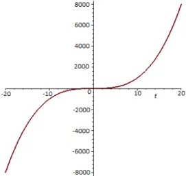
Set out in this study (29) equations are partial differential equations on twistorial generalized K¨ahler manifolds such that its solved with Maple computation program.
Fig. 1:Special values ofF1(t) =t3.
7 Discussion
It is well-known that a classical field theory explain the study of how one or more physical fields interact with matter which is used quantum and classical mechanics of physics branches. How the movement of objects in electrical, magnetically and gravitational fields force is very important. Because, the classical theory of electromagnetism deals with electric and magnetic fields and their interaction with each other and with charges and currents. An electromagnetic field is a physical field produced by electrically charged objects and their locations over time.
It is well-known that the motivation and one of the initial aims of twistor theory is to provide an adequate formalism for the union of quantum theory and general relativity. Twistor theory can also be used to solve non-linear differential
equations which are related to the self-duality equations that describe instantaneous in R4. In this study, the
Euler-Lagrange mechanical equations (29) derived on twistorial generalized K¨ahler manifolds may be suggested to deal with problems in electrical, magnetically and gravitational fields for the path of movement (Fig 1.) of defined space moving objects [23,24].
References
[1] R. Penrose, Twistor algebra. J. Math. Phys., 8, (1967), 345–366.
[2] R. Penrose, Twistor Theory, Its Aims and Achievements, Clarendon Press, Oxford, (1975), 268–407. [3] L. Freidela and S. Spezialeb, From Twistors to Twisted Geometries, http://arxiv.org/abs/1006.0199v1, (2010). [4] S. Speziale, Loop Quantum Gravity and Twisted Geometries, Zakopane, (2011).
[5] S. Santa-Cruz, Twistor Geometry for Hyperkahler Metrics on Complex Adjoint Orbits, Annals of Global Analysis and Geometry 15: 361–377, 1997.
[6] R. Albuquerque, Twistorial Constructions of Special Riemannian Manifolds, AIP Conference Proceedings, Vol. 1023 Issue 1, (2008).
[7] J. Davidov and O. Mushkarov, Twistor Spaces of Generalized Complex Structures, JGP, 56, (2006), 1623–1636.
[9] R. Pantilie, On a Class of Twistorial Maps, Differential Geometry and its Applications, 26, (2008), 366–376.
[10] S. Ianus¸S. Marchiafava, L. Ornea, R. Pantilie, Twistorial Maps Between Quaternionic Manifolds, arXiv:0801.4587v2, (2008). [11] M. Dunajski, Twistor Theory and Differential Equations, arXiv:0902.0274v2, (2009).
[12] S. Marchiafava, Twistorial Maps Between (para) Quaternionic Projective Spaces, Bull. Math. Soc. Sci. Math. Roumanie Tome, 52(100), No. 3, (2009), 321–332.
[13] Z. Kasap, Weyl-Euler-Lagrange Equations of Motion on Flat Manifold, Advances in Mathematical Physics, (2015), 1-16. [14] M. Tekkoyun, Mechanics Systems on Para-K¨ahlerian Manifolds of Constant J-Sectional Curvature,
http://arxiv.org/abs/0902.3569v1, (2009), 1-8.
[15] S. Cecotti, A. Neitzke, C. Vafa, Twistorial Topological Strings and a tt∗Geometry for N=2 Theories in 4d, arXiv:1412.4793v1, (2014).
[16] N. Nowaczyk, J. Niediek and M. Firsching, Basics of Complex Manifolds, (2009).
[17] W. Ballmann, Lectures on K¨ahler Manifolds, ESI Lectures in Mathematics and Physics, ISBN 978-3-03719-025-8, (2006). [18] D.J. Griffiths, Introduction to Electrodynamics. Prentice Hall. ISBN 0-13-805326-X, (1999).
[19] J. Klein, Escapes Variationnels et M´ecanique, Ann. Inst. Fourier, Grenoble,12(1962).
[20] A. Ibord, The Geometry of Dynamics, Extracta Mathematicable, Vol.11, Num.1,(1996), 80-105.
[21] M. de Leon and P.R. Rodrigues, Methods of Differential Geometry in Analytical Mechanics, Elsevier Sc. Pub. Com. Inc., Amsterdam,(1989).
[22] R. Abraham, J.E. Marsden and T. Ratiu, Manifolds Tensor Analysis and Applications, Springer,(2001).
[23] B. Thid´e, Electromagnetic Field Theory, (2012).