A Family of Stationary Solutions to the Euler
Equations and Generalized Solutions
JULIANACONCEIÇÃOPRECIOSO
Departamento de Matemática, Universidade Estadual Paulista, 15054-000, S.J.R. Preto, SP, Brazil email:[email protected]
ABSTRACT
In this work, we present a interesting family of stationary solutions for the Euler equations, which behaves in the same way that the approximated solutions presented in [6].
RESUMEN
En este trabajo, presentamos una familia interesante de soluciones estacionarias para las ecuaciones de Euler, que se comportan de la misma manera que las soluciones aproximadas presentadas en [6].
Key words and phrases:Euler equations, incompressible flows, generalized solutions.
1
Introduction
An ideal incompressible fluid moving insideD⊂Rnis classically described by a velocity field
u(t,x) and a pressure field p(t,x), subject to the classical Euler equations:
(
∂tu+(u· ∇)u+ ∇p=0
∇ ·u=0, (1.1)
with the boundary condition thatuis tangent to∂D.
In classical continuous mechanics [1], the motion of an incompressible inviscid fluid in a compact domainD⊂Rn can be seen as a geodesic on the group of all diffeomorphisms ofD with unit jacobian determinant,G(D). This set is included inS(D) the semigroup of all Borel mapshofDthat satisfy
ˆ
D
f(h(x))dx= ˆ
D
f(x)dx, ∀f∈C0(D).
For more details see [1], [2] or [6].
We will denote
V:=nu: [0,T]×D−→Rn such that u∈C0(Q), u(t,·)∈Li p(D)
uniformly in 0≤t≤T,divu=0, u(t,·)·nb¯¯ ∂D
=0o.
Note that the flow (t,x)7→g(t,x) describing the motion of fluid particles is defined by (
∂tg(t,x)=u(t,g(t,x))
g(0,x)=x. (1.2)
By Cauchy-Lipschitz theorem, for each u∈V, there is a unique solution to (1.2) and for each timetthe map g(t,x)=g(t,·)∈G(D). Then, by elementary calculations, the Euler equations can be replaced by the following equivalent equations:
(
∂2ttg(t,x)+ ∇p(t,g(t,x))=0 detDxg(t,x)=1.
(1.3)
Lets call (1.3) by the “Lagrangian formulation” of the Euler equations.
velocity field, it is natural to solve the problem to minimize the action
A(g)=1
2
ˆ T
0 ˆ
D
|∂tg(t,x)|2dxdt,
among all trajectories onG(D) connecting g(0,·)=I dand g(T,·)=h.
The corresponding system of PDE’s is the lagrangian formulation of the Euler equations (1.3).
Ebin and Marsden showed local existence and uniqueness for this problem, namely, ifh and Iare sufficiently close in a sufficiently high order Sobolev norm, then there is a unique geodesic connectingI dtoh, see [9]. In the large, uniqueness can fail. However, in [12], A. I. Shnirelman shows that existence of minimal geodesics may fail to a class of data.
To solve the problem to find minimal geodesics in a generalized sense, in particular for data h in Shnirelman class, was introduced suitable “Young measure", (see [15] and [18]) of different ways as in [4], [6], [12] and [13]. In [4], was used a concept that takes into account the dynamics of the particles. To each path t∈[0,T]7−→z(t)∈D, one associates the probability that it is followed by some material particle. More precisely, was proposed a notion of the generalized flow, as been a probability measure on setΩ=D[0,T]of all curves t∈[0,T]−→z(t)∈D, namely, a Borel probability measureµ, on product spaceΩ=D[0,T], such that each projectionµtfor 0≤t≤Tis a Lebesgue measure onD. The action in this context is express by
ˆ
Ω
ˆ T
0
1 2|z
′
(t)|2dµt(z)dt.
Brenier showed the existence of generalized solutions and, later in [5], the existence and uniqueness of the pressure gradient linked to them through a suitable Poisson equation, but did not obtain for them a complete set of equations beyond the classical Euler equations. However, in [6] it was possible. The problem to find minimal geodesics was reformulated in terms of a pair of measures associated to the fieldu, solution of the Euler equations, in the following way: Given a smooth trajectoryt∈[0,T]7→g(t,x)∈G(D), we define the measures (respectively nonnegative and vector-valued)
c(t,x,a)=δ(x−g(t,a)), m(t,x,a)=∂tg(t,a)δ(x−g(t,a)), (1.4)
defined onQ′=[0,T]×D×D. These measures satisfy
ˆ
D
c(t,x,a)da=1, (1.5)
∂tc+ ∇x·m=0, (1.6)
Moreover, the measuremis absolutely continuous with respect to c, with a densityv∈ L2(Q′,d c), so thatm=cv, and the action is given by
A(g)=1
2
ˆ 1
0 ˆ
D
|v(t,x,a)|2c(t,x,a)dxda,
or equivalently,A(g)=K[c,m], where
K[c,m] :=sup
X
{〈c,F〉 + 〈m,Φ〉}, (1.8)
where (c,m) is of the form (1.4) and
X= ½
(F,Φ)∈C0(Q′)׳C0(Q′)´n; F(t,x,a)+1
2|Φ(t,x,a)|
2≤0¾.
Then, Brenier defined the relaxed problem, as the problem to look for pairs of measures (c,m) that minimizeK[c,m] and are admissible in the sense of (1.5), (1.6) and (1.7), but do not necessarily satisfy (1.4).
Also was showed that, forD=[0,1]nand each datah∈S(D), the relaxed problem always has solutions (c,m) and that there is a unique locally bounded measure∇xpin the interior of Q=[0,T]×D, depending onlyh, such that
∂t(cv)+ ∇x(cv⊗v)+c∇xp=0,
holds in the sense of distributions on the interior ofQ′, wherecis a extension ofcfor which the productc(t,x,a)∇xp(t,x) is well-defined. Moreover, was showed that for anyh∈S([0,1]3) of the form
h(x1,x2,x3)=(H(x1,x2),x3),
that , for anyε>0, there is auε∈Vsuch that
K(uε)+
1
2ε||guε(T,·)−h||
2
L2(D)≤Iε(h)+ε,
whereIε(h)=infu∈v
½
K(u)+ 1
2ε||gu(T,·)−h||
2
L2(D)
¾ and
k(uε)=
1 2
ˆ T
0 ˆ
D
|uε(t,x)|2dxdt=
1 2
ˆ T
0 ˆ
D
|∂tgε(t,x)|2dxdt=A(gε).
In addition, the measures (cε,mε) associated withuε, through (1.4), converge, asε→0
to the generalized solutions of the relaxed problem. Moreover, the fieldsuεsatisfy
weakly, asεtends to zero. As observed in [6], with each solution (c,m) we may associated a measure-valued solutionµ, in the sense of DiPerna and Majda, by setting
ˆ
Q×Rd
f(t,x,ξ)dµ(t,x,ξ)= ˆ
Q′
f(t,x,v(t,x,a))d c(t,x,a),
for any continuous function f ∈Q×Rd with at most quadratic growth as ξ→ ∞. For more details, see [6] and [7].
In [4], Brenier shows explicit examples of non trivial generalized solutions. A typical example is when Dis the unit disk in 2D andh(x)= −x. We know that the problem of the minimal action has two trivial solutions g+(t,x)=eiπtxand g−(t,x)=e−iπtx with the same
pressure fieldp(x)=π
2|x|2
2 . We have another (generalized) solution (c,m) to the same problem which is given by
ˆ
Q′
f(t,x,a)c(t,x,a)dtdxda= ˆ
[0,1]×D
ˆ 1
0
f(t,G(t,a,θ),a)dθdtda,
ˆ
Q′
f(t,x,a)m(t,x,a)dtdxda= ˆ
[0,1]×D
ˆ 1
0
∂tG(t,a,θ)f(t,G(t,a,θ),a)dθdtda,
for all continuous function f, where
G(t,θ,a)=acos(πt)+¡1− |a|2¢ 1
2e2iπθsin(πt)∈D.
Note that each particle initially located ata∈Dsplits up along a circle of radius¡1− |a|2¢ 1 2
sin(πt), with centeracos(πt), that moves across the unit disk and shrinks down to the point −awhent=1.
In general, is very difficult to obtain explicit examples of non trivial generalized solu-tions and the explicit examples constructed by Brenier, are based on the model presented in [4], which takes in account a concept purely Lagrangian of Young measures, the so-called generalized flows. Beyond supplying an application of the model developed in [6], the results of this paper give an interesting information for the limit of a sequence of the stationary so-lutions, showing that they are associated with measures that satisfy the Euler equations in a specified weak sense. For another point of view, the results of the paper give example of as a sequence of highly oscillatory solutions still can have a limit that is solution in some sense. Namely, we exhibited a familyuε (which behavior as the“approximated solutions"
ar-gued above) such that whenε→0, the velocity field gets more and more oscillatory, but the measures (cε,mε) associated to the fielduεconverges to a solution (c,m) of the equations
ˆ
D
and
∂t(cv)+ ∇x(cv⊗v)+c∇xp=0.
Equivalent vector fields to those ones treaties in this work have been studied as appli-cation of high order essentially no oscillatory (ENO) schemes for smooth solutions of Navier-Stokes and Euler equations, (see [14]), in problems involving the Taylor-Green vortex, (see [8], [3] and [10]) and to explore a discrete singular convolution algorithm (DSC) for solving certain mechanics problems, (see [16] and [17]).
2
A Family of (Stationary) Solutions
In this work we consider the following family of stationary solutions to the Euler equations:
un(x,y)= µ
−cos(x)sin(n y),1
nsin(x)cos(n y),0 
,
pn(x,y)= −1
4 µ
cos(2x)+ 1
n2cos(2n y) 
.
Note that,|D pn(x,y)| ≤C, and whenn goes to infinity the pressure field strongly con-verges top(x,y)= −1
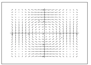
4cos(2x). Then, is easy verify that (un· ∇)un+ ∇p→0, whenn→ ∞. For a moment, let us observe the behavior of familyun. Forn=1 we have,
u1(x,y)=(−cos(x)sin(y),sin(x)cos(y),0)
and (
˙
x= −cos(x)sin(y) ˙
y=sin(x)cos(y). (2.1)
Then, we have ( ˙x, ˙y)=(0,0)⇔(x,y)=³(2k+1)π
2,(2l+1) π 2 ´
or (kπ,lπ), wherek,l∈Z, (see Figure 1).
Forn=2 we have, ( ˙x, ˙y)=(0,0)⇔(x,y)=³(2k+1)π
2,(2l+1) π 4 ´
or µ
kπ,lπ 2
, wherek,l∈Z,
(see Figure 2).
Thus, for n we have, ( ˙x, ˙y)=(0,0)⇔(x,y)=³(2k+1)π 2,(2l+1)
π 2n
´ or
µ kπ,lπ
n 
, where k,l∈Z.
Note that, whenn→ ∞the velocity field gets more and more oscillatory. In the next
sec-tion we will show that the measures (cn,mn) defined bycn(t,x,a)=δ¡x−gun(t,a)
¢
,mn(t,x,a)= un(t,x)δ(x−gun(t,a)) converges to the solution (c,m) of the equations:
ˆ
D
–2 –1 0 1 2
y
–2 –1 1 2
x
Figure 1: Phase portrait of the velocity fieldu1(x,y)=(−cos(x)sin(y),sin(x)cos(y),0)
–2 –1 0 1 2
y
–2 –1 1 2
x
Figure 2: Phase portrait of the velocity fieldu2(x,y)= µ
−cos(x)sin(2y), 1
2sin(x)cos(2y),0 
∂tc+ ∇x·m=0 (2.3)
∂t(cv)+ ∇x·(cv⊗v)+c∇xp=0, (2.4)
3
The Limite
(
c
,
m
)
In this section we build explicitly the limite (c,m). For this, in first we rewrite the field
un(x,y)= µ
−cos(x)sin(n y),1
nsin(x)cos(n y),0 
as
un(x,y)= µ
u11(x,n y),1 nu
2
1(x,n y),0
¶ ,
where
u11(x,n y)= −cos(x)sin(n y) and u21(x,n y)=sin(x)cos(n y).
Of here in ahead, we will omit third coordinate of the fieldsu′ns. We also observe that the field has period 2π. Now, we define
(
x=x(t,γ,δ)
y=y(t,γ,δ)
the solution of
dx dt=u
1
1(x,y)=cos(x)sin(y)
d y dt=u
2
1(x,y)=sin(x)cos(y)
x(0,γ,δ)=γ
y(0,γ,δ)=δ.
(3.1)
Let be 0≤i≤n−1, 0≤α1≤2π, and 2πi
n ≤α2≤ 2π
n (i+1), wherei,n∈N. This is: • forn=1,i=0 and we have 0≤α2≤2π.
• forn=2, 0≤i≤1 and we have (
0≤α2≤π, if i=0
π≤α2≤2π, if i=1.
• forn=k, 0≤i≤k−1 and we have
0≤α2≤2π
k , if i=0 2π
k ≤α2≤ 4π
k , if i=1 ...
2π(k−1)
α 2
α2
α1 α
1
0 0
2π 2π
2π 2π
n=1
π
n=2
α 2
α 1 0
π 2
2π π
n=k
k 2π k 2π(k-1)
Figure 3:
Then,icounts the cells (in the vertical line) from 0 to 2πfor eachn, as we can observe in Figure 3.
Now, we define
xni(t,α1,α2) :=x
µ t,α1,n
µ
α2−2πi
n ¶¶
yni(t,α1,α2) :=1
ny µ
t,α1,n
µ
α2−2πi
n ¶¶
+2πi n .
(3.2)
Note that, by the definition above
• forn=1, we havei=0, thus (
x10(t,α1,α2) :=x(t,α1,α2),
y01(t,α1,α2) :=y(t,α1,α2).
• forn=2, we have 0≤i≤1, thus
x02(t,α1,α2) :=x(t,α1,2α2)
y20(t,α1,α2) :=1
2y(t,α1,2α2)
,if i=0
and
x21(t,α1,α2) :=x(t,α1,2(α2−π))
y12(t,α1,α2) :=1
2y(t,α1,2(α2−π))+π
,if i=1.
• forn=k, we have 0≤i≤k−1, thus
x0k(t,α1,α2) :=x(t,α1,kα2)
y0k(t,α1,α2) :=1
ky(t,α1,kα2)
.. .
xkk−1(t,α1,α2) :=x
µ t,α1,k
µ
α2−2(k
−1)π
k ¶¶
y2k−1(t,α1,α2)
:=1 ky
µ t,α1,k
µ
α22(k
−1)π
k ¶¶
+2(k−1)π k
,if i=k−1.
Then, we conclude that 0≤xin≤2π,2πi
n ≤y i n≤
2π(i+1) n and
xin(0,α1,α2)=x µ
0,α1,n µ
α2−2πi n
¶¶ =α1
yni(0,α1,α2)=1 ny
µ 0,α1,n
µ
α2−2πi n
¶¶ +2πi
n =α2.
Moreover, by (3.2) we have
dxin
dt (t,α1,α2)= dx
dt µ
t,α1,n
µ
α2−2πi
n ¶¶
d yni
dt (t,α1,α2)= 1 n
d y dt µ
t,α1,n
µ
α2−2πi
n
¶¶ (3.3)
Therefore, by (3.1) and (3.3)
dxin
dt = u
1 1
µ x
µ t,α1,n
µ
α2−2πi
n ¶¶
,y µ
t,α1,n
µ
α2−2πi
n ¶¶¶
= u11³xin(t,α1,α2),n yni(t,α1,α2)−2πi ´
= u11³xin(t,α1,α2),n yni(t,α1,α2) ´
= u1n³xin(t,α1,α2),yni(t,α1,α2)
´ ,
and
d yni dt = 1 nu 2 1 µ x µ t,α1,n
µ
α2−2πi
n ¶¶
,y µ
t,α1,n
µ
α2−2πi
n ¶¶¶ = 1 nu 2 1 ³
xni(t,α1,α2),n yni(t,α1,α2)−2πi´
= 1 nu
2 1
³
xni(t,α1,α2),n yni(t,α1,α2) ´
= u2n³xin(t,α1,α2),yni(t,α1,α2) ´
.
Now defining (
xn(t,α1,α2) :=xin(t,α1,α2)
yn(t,α1,α2) :=yni(t,α1,α2)
if 2πi n ≤α2≤
2π(i+1)
we conclude that
dxn
dt (t,α1,α2)=u
1
n(xn(t,α1,α2),yn(t,α1,α2)) d yn
dt (t,α1,α2)=u
2
n(xn(t,α1,α2),yn(t,α1,α2))
xn(0,α1,α2)=α1
yn(0,α1,α2)=α2.
(3.4)
In the remain of the work, for simplicity, we will use the following notation:Di=(0,2π)i= (0,2π)× · · · ×(0,2π),itimes, wherei=1,· · ·,4. Now, we are ready to show the following result:
Theorem 3.1. Consider(xn,yn)solution of (3.4). Let (
cn(t,x,y,α1,α2)=δ((x,y)−(xn(t,α1,α2),yn(t,α1,α2)))
mn(t,x,y,α1,α2)=un(x,y)δ((x,y)−(xn(t,α1,α2),yn(t,α1,α2))).
Then,
〈ϕ,cn〉 → 1 2π
ˆ
D3 ˆ T
0
ϕ(x(t,α1,β2),γ,α1,γ,t)dtdα1dβ2dγ
and〈φ,mn〉 →
1 2π
ˆ
D3 ˆ T
0 φ
1(x(t,α
1,β2),γ,α1,γ,t)u11(x(t,α1,β2),y(t,α1,β2))dtdα1dβ2dγ,
whenever n→ ∞,for any ϕ∈C∞
0 (D4×(0,T))andφ∈
¡ C∞
0 (D4×(0,T))
¢2
.
Proof. Letϕ∈C0∞(D4×(0,T)) and
cn(t,x,y,α1,α2)=δ((x,y)−(xn,yn)(t,α1,α2))
then, we have
〈ϕ,cn〉 =
ˆ
D2 ˆ T
0
ϕ(xn(t,α1,α2),yn(t,α1,α2),α1,α2,t)dtdα1dα2
=
nX−1
i=0 ˆ 2π
n(i+1)
2π ni
ˆ 2π
0 ˆ T
0 ϕ
³
xin(t,α1,α2),yni(t,α1,α2),α1,α2,t´dtdα1dα2
=
nX−1
i=0
ˆ 2nπ(i+1)
2π ni
ˆ 2π
0 ˆ T
0
ϕ
µ x
µ t,α1,n
µ
α2−2πi
n ¶¶
,
1 ny
µ t,α1,n
µ
α2−2πi
n ¶¶
+2πi
n ,α1,α2,t 
Now, makeβ2=n µ
α2−2πi n
=nα2−2πi, namely,α2=β2 n +
2πi
n . Then, we have
〈ϕ,cn〉 = nX−1
i=0 ˆ D2 ˆ T 0 ϕ µ
x(t,α1,β2),1
ny(t,α1,β2)+ 2πi
n ,
α1,β2
n + 2πi
n ,t 
dtdα1dβ2
n = An+Bn,
where
An= 1 2π
nX−1
i=0 Ã ˆ D2 ˆ T 0 ϕ µ
x(t,α1,β2),2πi
n ,α1, 2πi
n ,t 
dtdα1dβ2
! 2π
n (3.5)
and
Bn = nX−1
i=0 1 n ˆ D2 ˆ T 0 · ϕ µ
x(t,α1,β2),1
ny(t,α1,β2)+ 2πi
n ,α1,
β2
n + 2πi
n ,t 
−ϕ
µ
x(t,α1,β2),2πi
n ,α1, 2πi
n ,t ¶¸
dtdα1dβ2.
Note that, by Mean Value Theorem, we have ¯
¯ ¯ ¯ϕ
µ
x(t,α1,β2),1
ny(t,α1,β2)+ 2πi
n ,α1,
β2
n + 2πi
n ,t 
−
−ϕ
µ
x(t,α1,β2),2πi
n ,α1, 2πi
n ,t ¶¯¯ ¯ ¯= ¯ ¯ ¯ ¯ ∂ϕ ∂y 1
ny(t,α1,α2)+
∂ϕ ∂β2 β2 n ¯ ¯ ¯ ¯≤ ≤ ï ¯ ¯ ¯ ¯ ¯ ¯ ¯ ∂ϕ ∂y ¯ ¯ ¯ ¯ ¯ ¯ ¯ ¯
L∞((0,2π)4×(0,T))
|y(t,α1,α2)|
n + ¯ ¯ ¯ ¯ ¯ ¯ ¯ ¯ ∂ϕ ∂β2 ¯ ¯ ¯ ¯ ¯ ¯ ¯ ¯
L∞((0,2π)4×(0,T)) |β2|
n !
≤
≤2π n µ¯¯ ¯ ¯ ¯ ¯ ¯ ¯ ∂ϕ ∂y ¯ ¯ ¯ ¯ ¯ ¯ ¯ ¯ L∞ + ¯ ¯ ¯ ¯ ¯ ¯ ¯ ¯ ∂ϕ ∂β2 ¯ ¯ ¯ ¯ ¯ ¯ ¯ ¯ L∞ ¶ ≤2π
n ∥Dϕ∥L∞.
Then, we obtain
|Bn| ≤ nX−1
i=0 1 n ˆ D2 ˆ T 0 ¯ ¯ ¯ ¯ · ϕ µ
x(t,α1,β2),1
ny(t,α1,β2)+ 2πi
n ,α1,
β2
n + 2πi
n ,t 
−ϕ
µ
x(t,α1,β2),2πi
n ,α1, 2πi
n ,t ¶¸¯¯
¯
¯dtdα1dβ2
≤
nX−1
i=0
1 n
2π
n ∥Dϕ∥L∞
ˆ 2π 0 ˆ 2π 0 ˆ T 0
dtdα1dβ2
= 2π
n ∥Dϕ∥L∞4π
2T−2π
n2∥Dϕ∥L∞4π
2T
≤ 2π
n ∥Dϕ∥L∞4π
Therefore,Bn→0, whenn→ ∞.
Now, define the functionψby
ψ(γ) := ˆ
D2 ˆ T
0 ϕ(
x(t,α1,β2),γ,α1,γ,t)dtdα1dβ2
thus, we rewrite (3.5) as
An= 1 2π
nX−1
i=0
ψ
µ2πi
n ¶2π
n = 1 2π
nX−1
i=0
ψ
µ2πi
n
¶µ2π(i+1)
n − 2πi
n 
.
By this form, if γi= 2πi
n then, ©
γ0,γ1,· · ·,γnª is a partition of the (0,2π) and An =
1 2π
nX−1
i=0
ψ(γi)¡γi+1−γi¢is a Riemann sum. Therefore,
An→ 1 2π
ˆ 2π
0
ψ(γ)dγ,
whenn→ ∞. Then, we conclude that
〈ϕ,cn〉 → 1 2π
ˆ
D3 ˆ T
0
ϕ(x(t,α1,β2),γ,α1,γ,t)dtdα1dβ2dγ,
whenn→ ∞, for anyϕ∈C∞0 (D4×(0,T)).
Now, considerφ∈¡C∞0 (D4×(0,T))¢2and let
mn = un(x,y)δ((x,y)−(xn(t,α1,α2),yn(t,α1,α2)))
= µ
u11(x,n y),1 nu
2 1(x,n y)
δ((x,y)−(xn(t,α1,α2),yn(t,α1,α2))).
Then, we obtain
〈φ,mn〉 =
ˆ
D2 ˆ T
0
φ(xn(t,α1,α2),yn(t,α1,α2),α1,α2,t)
h
u11(xn(t,α1,α2),
n yn(t,α1,α2)),1
nu
2
1(xn(t,α1,α2),n yn(t,α1,α2))
i
dtdα1dα2
=
nX−1
i=0
ˆ 2nπ(i+1)
2π ni
ˆ 2π
0 ˆ T
0 φ(
xin(t,α1,α2),yni(t,α1,α2),α1,α2,t)
h
u11(xni(t,α1,α2),n yni(t,α1,α2)), 1 nu
2
1(xin(t,α1,α2),
n yni(t,α1,α2))
i
and therefore, makingβ2=n µ
α2−2πi n
we have
〈φ,mn〉 = nX−1
i=0 ˆ D2 ˆ T 0 1 nφ
1µx(t,α 1,β2),1
ny(t,α1,α2)+ 2πi
n ,α1,
β2
n + 2πi
n ,t 
u11(x(t,α1,β2),y(t,α1,β2))dtdα1dβ2+
+
nX−1
i=0 ˆ D2 ˆ T 0 1 n2φ
2µx(t,α 1,β2),1
ny(t,α1,α2)+ 2πi
n ,α1, 2πi
n ,t 
u21(x(t,α1,β2),y(t,α1,β2))dtdα1dβ2
= A1n+B1n+A2n+B2n,
where,
A1n = 1
2π nX−1
i=0
³ˆ D2 ˆ T 0 1 nφ
1µx(t,α
1,β2),2πi
n ,α1, 2πi
n ,t 
u11(x(t,α1,β2),y(t,α1,β2))dtdα1dβ2
´ 2π,
A2n = 1
2πn nX−1
i=0 ³ˆ D2 ˆ T 0 1 nφ
2µx(t,α
1,β2),2πi
n ,α1, 2πi
n ,t 
u21(x(t,α1,β2),y(t,α1,β2))dtdα1dβ2
´ 2π,
B1n =
nX−1
i=0 ˆ D2 ˆ T 0 1 n · φ1 µ
x(t,α1,β2),1
ny(t,α1,β2)+ 2πi
n ,
α1,β2
n + 2πi
n ,t 
−φ1
µ
x(t,α1,β2),2πi
n ,α1, 2πi
n ,t ¶¸
u11(x(t,α1,β2),y(t,α1,β2))dtdα1dβ2,
B2n =
nX−1
i=0 ˆ D2 ˆ T 0 1 n2 · φ2 µ
x(t,α1,β2),1
ny(t,α1,β2)+ 2πi
n ,α1,
β2
n + 2πi
n ,t 
−φ2
µ
x(t,α1,β2),2πi
n ,α1, 2πi
n ,t ¶¸
u21(x(t,α1,β2),y(t,α1,β2))dtdα1dβ2,
As we seen before, we conclude that ¯
¯ ¯ ¯φi
µ
x(t,α1,β2),1
ny(t,α1,β2)+ 2πi
n ,α1,
β2
n + 2πi
n ,t 
−
−φi
µ
x(t,α1,β2),2πi
n ,α1, 2πi
n ,t ¶¯¯
¯ ¯≤
2π
Thus, we have the estimate
|B1n| ≤
nX−1
i=0
1 n ˆ D2 ˆ T 0 ¯ ¯ ¯ ¯φ1
µ
x(t,α1,β2),1
ny(t,α1,β2)+ 2πi
n ,α1,
β2
n + 2πi
n ,t 
−φ1
µ
x(t,α1,β2),2πi
n ,α1, 2πi
n ,t ¶¯¯
¯
¯|u11(x(t,α1,β2),y(t,α1,β2))|dtdα1dβ2,
≤ 2π
n ∥Dφ∥L∞4π
2TC.
Therefore,B1n→0, whenn→ ∞. Now, we go to study the termB2n.
|B2n| ≤
nX−1
i=0 1 n2 ˆ D2 ˆ T 0 ¯ ¯ ¯ ¯φ2
µ
x(t,α1,β2),1
ny(t,α1,β2)+ 2πi
n ,α1,
β2
n + 2πi
n ,t 
−φ2
µ
x(t,α1,β2),2πi
n ,α1, 2πi
n ,t ¶¯¯
¯
¯|u21(x(t,α1,β2),y(t,α1,β2))|dtdα1dβ2
≤ 2π
n2 ∥Dφ∥L∞4π
2TC,
and, therefore, alsoB2n→0, whenn→ ∞.
Defining the functionψby
ψi(γ) := ˆ
D2 ˆ T
0 φ
i(x(t,α
1,β2),γ,α1,γ,t)ui1(x(t,α1,β2),y(t,α1,β2))dtdα1dβ2,
i=1,2, we obtain,
A1n = 1
2π nX−1
i=0
ψ1
µ2πi
n ¶2π
n
= 1
2π nX−1
i=0
ψ1
µ2πi
n
¶µ2π(i+1)
n − 2πi
n 
.
By this form, if γi= 2πi
n then, ©
γ0,γ1,· · ·,γn ª
is a partition of the (0,2π) and A1n =
1 2π
nX−1
i=0
ψ1(γi) ¡
γi+1−γi ¢
is a Riemann sum. Therefore,
A1n→ 1
2π
ˆ 2π
0
ψ1(γ)dγ, when n→ ∞.
For the last term, we have that
A2n = 1
2πn nX−1
i=0
ψ2
µ2πi
n ¶2π
= 1
2πn nX−1
i=0
ψ2
µ2πi
n
¶µ2π(i+1)
n − 2πi
n 
,
and therefore,A2n→0, whenn→ ∞.
Then, we conclude that
〈φ,mn〉 →
1 2π
ˆ
D3 ˆ T
0
φ1(x(t,α1,β2),γ,α1,γ,t)u11(x(t,α1,β2),y(t,α1,β2))dtdα1dβ2dγ,
whenn→ ∞, for anyφ∈¡C∞0 (D4×(0,T))¢2.
By the last theorem we can conclude that
〈ϕ,cn〉 → 1 2π
ˆ
D3 ˆ T
0
ϕ(x(t,α1,β2),γ,α1,γ,t)dtdα1dβ2dγ
and〈φ,mn〉 →
1 2π
ˆ
D3 ˆ T
0
φ1(x(t,α1,β2),γ,α1,γ,t)u11(x(t,α1,β2),y(t,α1,β2))dtdα1dβ2dγ,
whenever n→ ∞, for any
ϕ∈C∞0 (D4×(0,T)) andφ∈¡C0∞(D4×(0,T))¢2.
Now, note that
2π〈ϕ,cn〉 →
ˆ
D3 ˆ T
0
ϕ(x(t,α1,β2),γ,α1,γ,t)dtdα1dβ2dγ
is equivalent to
ˆ 2π
0
〈ϕ,cn〉dβ2→ ˆ
D3 ˆ T
0 ϕ(
x(t,α1,β2),γ,α1,γ,t)dtdα1dγdβ2
and, therefore,
ˆ 2π
0
"
〈ϕ,cn〉 −
ˆ
D2 ˆ T
0
ϕ(x(t,α1,β2),γ,α1,γ,t)dtdα1dγ
#
dβ2→0.
Then, we conclude that
〈ϕ,cn〉 →
ˆ
D2 ˆ T
Of completely analogous way, we also conclude that
〈φ,mn〉 →
ˆ
D2 ˆ T
0
φ1(x(t,α1,β2),γ,α1,γ,t)u11
¡
x(t,α1,β2),y(t,α1,β2)¢dtdα1dγ.
Thus, the limite (c,m) is given by (
c(x,y,α1,α2,t)=δ¡(x,α2)−(x(t,α1,β2),y)¢
m(x,y,α1,α2,t)=δ¡(x,α2)−(x(t,α1,β2),y)¢¡u11(x,y(t,α1,β2)),0¢.
(3.6)
4
Solution to the Relaxed Euler Equations
In this section we will conclude our work showing that the pair (c,m), build in the before section, satisfy the relaxed Euler equations.
Theorem 4.1. The pair of measures (c,m) defined in (3.6) satisfy the following equations
ˆ
D2
c(t,x,y,α1,α2)dα1dα2=1, ∂tc+ ∇ ·m=0, ∂t(cv)+ ∇ ·(cv⊗v)+c∇p=0.
in the sense of distributions.
Proof. Note that
〈1,c〉 = ˆ
D2 ˆ T
0
dtdα1dα2= ˆ
D2 ˆ T
0
dtdxd y.
Then, we obtain
ˆ
D2 ˆ T
0
µˆ
D2
c(t,x,y,α1,α2)dα1dα2−1
dtdxd y=0
and, therefore,
ˆ
D2
c(t,x,y,α1,α2)dα1dα2=1.
Now, we will show that pair (c,m) satisfy the equation ∂tc+ ∇ ·m=0. Consider ϕ∈ C∞0(D4×(0,T)), thus
〈ϕ(x,y,α1,α2,t),∂tc(t,x,y,α1,α2)+ ∇(x,y)·m(t,x,y,α1,α2)〉 =
= − ˆ
D2 ˆ T
0
∂tϕ(x(t,α1,β2),y,α1,y,t)dtdα1d y
− ˆ
D2 ˆ T
0 ∂xϕ(x(t,α1,β2),y,α1,y,t)u 1
= − ˆ
D2 ˆ T
0
∂t ¡
ϕ(x(t,α1,β2),y,α1,y,t)¢dtdα1d y
= − ˆ
D2 ¡
ϕ(α1,y,α1,y,T)−ϕ(β2,y,α1,y,0)¢dα1d y=0.
Finally, we will show that the pair (c,m) also satisfy the equation∂t(cv)+∇·(cv⊗v)+c∇p=
0. First note that£d iv(x,y)(u⊗u)¤i=uid iv(x,y)u+u·∇(x,y)ui=u·∇(x,y)ui, becaused iv(x,y)u=0.
Letϕ∈¡C∞0 (D4×(0,T))¢2, then
〈ϕ1(x,y,α1,α2,t),∂t¡c(t,x,y,α1,α2)v1(x,y,α1,α2,t)〉 +
+ 〈ϕ1(x,y,α1,α2,t),∇(x,y)·(c(t,x,y,α1,α2)v(x,y,α1,α2,t)⊗v(x,y,α1,α2,t))1〉
+ 〈ϕ1(x,y,α1,α2,t),c(x,y,α1,α2,t)∂xp(x,y)〉 =
= − ˆ
D2 ˆ T
0
u11(x(t,α1,β2),y(t,α1,β2))∂tϕ1(x(t,α1,β2),y,α1,y,t)dtdα1d y
− ˆ
D2 ˆ T
0
£
u11(x(t,α1,β2),y(t,α1,β2))¤2∂xϕ1(x(t,α1,β2),y,α1,y,t)dtdα1d y
+ ˆ
D2 ˆ T
0
∂xp(x(t,α1,β2),y)ϕ1(x(t,α1,β2),y,α1,y,t)dtdα1d y
= − ˆ
D2 ˆ T
0
u11(x(t,α1,β2),y(t,α1,β2))∂t£ϕ1(x(t,α1,β2),y,α1,y,t)¤dtdα1d y
+ ˆ
D2 ˆ T
0
£
u11(x(t,α1,β2),y(t,α1,β2))¤2∂xϕ1(x(t,α1,β2),y,α1,y,t)dtdα1d y
− ˆ
D2 ˆ T
0
£
u11(x(t,α1,β2),y(t,α1,β2))¤2∂xϕ1(x(t,α1,β2),y,α1,y,t)dtdα1d y
+ ˆ
D2 ˆ T
0 ∂xp(x(t,α1,β2),y)ϕ 1(x(t,α
1,β2),y,α1,y,t)dtdα1d y
= ˆ
D2 ˆ T
0
∂t£u11(x(t,α1,β2),y(t,α1,β2))¤ϕ1(x(t,α1,β2),y,α1,y,t)dtdα1d y
+ ˆ
D2 ˆ T
0
∂xp(x(t,α1,β2),y)ϕ1(x(t,α1,β2),y,α1,y,t)dtdα1d y
= ˆ
D2 ˆ T
0
£
∂xu11(x(t,α1,β2),y(t,α1,β2))∂tx(t,α1,β2)
+∂yu11(x(t,α1,β2),y(t,α1,β2))∂ty(t,α1,β2)¤ϕ1(x(t,α1,β2),y,α1,y,t)dtdα1d y
+ ˆ
D2 ˆ T
0
∂xp(x(t,α1,β2),y)ϕ1(x(t,α1,β2),y,α1,y,t)dtdα1d y
= ˆ
D2 ˆ T
0
u11(x(t,α1,β2),y(t,α1,β2))ϕ1(x(t,α1,β2),y,α1,y,t)dtdα1d y
+ ˆ
D2 ˆ T
0
∂xp(x(t,α1,β2),y)ϕ1(x(t,α1,β2),y,α1,y,t)dtdα1d y.
Since thatp(x)= −1
4cos(2x) we have that∂xp= 1
2sin(2x) and then,
∂xp(x(t,α1,β2),y)=∂xp(x(t,α1,β2),y(x(t,α1,β2)).
Therefore, we conclude that
〈ϕ1(x,y,α1,α2,t),∂t¡c(t,x,y,α1,α2)v1(x,y,α1,α2,t)〉 +
+ 〈ϕ1(x,y,α1,α2,t),∇(x,y)·(c(t,x,y,α1,α2)v(x,y,α1,α2,t)⊗v(x,y,α1,α2,t))1〉 +
+ 〈ϕ1(x,y,α1,α2,t),c(x,y,α1,α2,t)∂xp(x,y)〉 =
= ˆ
D2 ˆ T
0
£
∇(x,y)u11(x(t,α1,β2),y(t,α1,β2))u11(x(t,α1,β2),y(t,α1,β2))
+∂xp(x(t,α1,β2),y(t,α1,β2))¤ϕ1(x(t,α1,β2),y,α1,y,t)dtdα1d y.
Now, note thatu11(x,n y)= −cos(x)sin(n y) andu21(x,n y)=sin(x)cos(n y), namely,u11(x,z)= −cos(x)sin(z) andu21(x,z)=sin(x)cos(z), wherez=n y. Then,
∇u11·u1= −sin(x)cos(x)= −1
2sin(2x), and, therefore,
∇u11·u1+∂xp= − 1
2sin(2x)+ 1
2sin(2x)=0. Then,
∇(x,y)u11¡x(t,α1,β2),y(t,α1,β2)¢·u1(x(t,α1,β2),y(t,α1,β2))+
+∂xp(x(t,α1,β2),y(t,α1,β2))=0
and we can conclude that the pair of measures (c,m=cv) satisfy
∂t(cv)+ ∇ ·(cv⊗v)+c∇p=0.
Acknowledgement.
References
[1] ARNOLD, V.I.,Sur la Géométrie Différentielle des Groupes de Lie de Dimension Infine et ses Applications à L’Hidrodynamique, Ann. Inst. Fourier,16, 319–361, 1966.
[2] ARNOLD, V.I. AND KHESIN, B., Topological Methods in Hidrodynamics, Annu. Rev. Fluid Mech.,24, 145–166, 1992.
[3] BENSOW, R.E., LARSON, M.G. AND VESTERLUND, P.,Vorticity-strain residual-based turbulence modelling of the Taylor-Green vortex, Int. J. Numer. Meth. Fluids,54, 745– 756, 2007.
[4] BRENIER, Y.,The Least Action Principle and the Related Concept of Generalized Flows for Incompressible Perfect Fluids, Journal of the American Mathematical Society, Vol. 2, Number 2, 225–255, 1989.
[5] BRENIER, Y.,The Dual Least Action Problem for an Ideal, Incompressible Fluid, Arch.
Rational Mech. Anal.,122, Number 4, 323–351, 1993.
[6] BRENIER, Y.,Minimal Geodesics on Groups of Volume-Preserving Maps and General-ized Solutions of the Euler Equations, CPAM 52, 411–452, 1999.
[7] DIPERNA, R.ANDMAJDAA.,Oscillations and Concentrations in Weak Solutions of the Incompressible Fluid Equations, Comm. Math. Phys.,108, 667–689, 1987.
[8] DON, W.-S, GOTTLIEB, D., JAMESON, L., SCHILLING, O.ANDSHU, C.-W.,Numerical Convergence Study of Nearly-Incompressible, Inviscid Taylor-Green Vortex Flow, Jour-nal of Scientific Computing,24, 569–595, 2005.
[9] EBIN, D.G.ANDMARSDENJ.,Groups of Diffeomorphisms and the Motion of an Incom-pressible Fluid, Ann. of Math.,92, 102–163, 1970.
[10] LEE,H.AND SOHRABS.H.,Hydrodynamic Aspects of Premixed Flame Stripes in Two-Dimensional Stagnation-Point Flows, Combustionand Flame,101, 441–451, 1995.
[11] PRECIOSO, J.C.,Equações relaxadas para hidrodinâmica ideal, não homogênea, Tese de doutorado, IMECC-UNICAMP, 2005.
[12] SHNIRELMAN, A.I.,The Geometry of the Groups of Diffeomorphisms and the Dynamics of an Ideal Incompressible Fluid, Mat. Sb (N.S.) 128(170), 82–109,144, 1985.
[13] SHNIRELMAN, A.I., Generalized Fluid Flows, their Aproximation and Applications,
Geom. Funct. Anal.,4, 586–620, 1994.
[15] TARTAR, L.,The Compensated Compactness Method Applied to Systems of Conserva-tion Laws. Systems of Nonlinear Partial Differential EquaConserva-tions, (Oxford, 1982), 263–285. NATO Adv. Sci. Inst. Ser. C: Math. Phys. Sci., 111. Reidel, Dordrecht-Boston, 1983.
[16] WAN, D.C., WEI, G.W.ANDZHOU, Y.C.,Numerical solution of incompressible flows by discrete singular convolution, Int. J. Numer. Meth. Fluids,38, 789–810, 2002.
[17] WEI, D.C., WEI,A new algorithm for solving some mechanical problems, Comput. Meth-ods Appl. Mech. Engrg.,190, 2017–2030, 2001.