Y.-F. Chen and A. Rezine (Eds.): The 12th INFINITY Workshop.
EPTCS 39, 2010, pp. 63–76, doi:10.4204/EPTCS.39.5 c B. Boigelot, J. Brusten, J.-F. Degbomont
Bernard Boigelot Julien Brusten† Jean-Franc¸ois Degbomont
Institut Montefiore, B28 Universit´e de Li`ege B-4000 Li`ege, Belgium
{boigelot,brusten,degbomont}@montefiore.ulg.ac.be
This paper addresses the symbolic representation of non-convex real polyhedra, i.e., sets of real vec-tors satisfying arbitrary Boolean combinations of linear constraints. We develop an original data structure for representing such sets, based on an implicit and concise encoding of a known structure, the Real Vector Automaton. The resulting formalism provides a canonical representation of poly-hedra, is closed under Boolean operators, and admits an efficient decision procedure for testing the membership of a vector.
1
Introduction
Algorithms and data structures for handling systems of linear constraints are extensively used in many areas of computer science such as computational geometry [13], optimization theory [24], computer-aided verification [10, 15], and constraint programming [23]. In this paper, we consider systems defined by arbitrary finite Boolean combinations of linear constraints over real vectors. Intuitively, a non-trivial linear constraint in then-dimensional space describes either a(n−1)-plane, or a half-space bounded by such a plane. A Boolean combination of constraints thus defines a region of space delimited by planar boundaries, that is, apolyhedron(also calledn-polytope).
Our goal is to develop an efficient data structure for representing arbitrary polyhedra, as well as asso-ciated manipulation algorithms. Among the requirements, one should be able to build representations of elementary polyhedra (such as the set of solutions of individual constraints), to apply Boolean operators in order to combine polyhedra, and to test their equality, inclusion, emptiness, and whether a given point belongs or not to a polyhedron.
A typical application consists in representing objects in a 3D modeling tool, in which shapes are approximated by polyhedral meshes. By applying Boolean operators, the user can modify an object, for instance, drilling a circular hole amounts to computing the Boolean difference between the object and a polyhedron approximating a cylinder. This application requires an efficient implementation of Boolean operations: A local modification performed on a complex object should ideally only affect a small part of its representation.
Another application (actually our primary motivation for studying this problem) is the symbolic representation of the reachable data values computed during the state-space exploration of programs. In this setting, a reachable set is computed iteratively, by repeatedly adding new sets of values to an initial set, and termination is detected by checking that the result of an exploration step is included in the set of values that have already been obtained. In this application, it is highly desirable for a representation of a set to be independent from the history of its construction, since reachable sets often
∗This work is supported by theInteruniversity Attraction PolesprogramMoVESof the Belgian Federal Science Policy
Office, and by the grant 2.4530.02 of the Belgian Fund for Scientific Research (F.R.S.-FNRS).
have simple structures, but are computed as the result of long sequences of operations. We are particularly interested inlinear hybrid systems[2], for which symbolic state-space exploration algorithms have been developed [1, 16], requiring efficient data structures for representing and manipulating systems of linear constraints. Existing representations either fail to be canonical [15, 17], or impose undue restrictions on the linear constraints that can be handled [11].
For some restricted classes of systems of linear constraints, data structures with good properties are already well known. Consider for instance conjunctions of linear constraints, which correspond to convex polyhedra. A convex polyhedron can indifferently be represented by a list of its bounding constraints, or by a finite set of vectors (its so-called vertices and extremal rays) that precisely characterize its shape [22]. An efficiently manageable representation is obtained by combining the bounding constraints and the vertices and rays of a polyhedron into a single structure [10, 19, 3].
There are several ways of obtaining a representation suited for arbitrary combinations of linear con-straints. A first one is to represent a set by a logical formula in additive real arithmetic. This approach is not efficient enough for our intended applications, since testing set emptiness, equality, or inclusion become NP-hard problems [12]. A second strategy is to decompose a non-convex polyhedron into an explicit union of convex polyhedra (which may optionally be required to be pairwise disjoint). The main disadvantage of this method is that a set can generally be decomposed in several different ways, and that checking whether two decompositions correspond to the same set is costly. Moreover, simplifying a long list of convex polyhedra into an equivalent shorter union is a difficult operation.
Another solution is to use automata [8]. The idea is to encoden-dimensional vectors as words over a given alphabet, and to represent a set of vectors by a finite-state machine that accepts the language of their encodings. This technique presents several advantages. First, with some precautions, computing Boolean combinations of sets reduces to applying the same operators to the languages accepted by the automata that represent them, which is algorithmically simple. Second, provided that one employs de-terministic automata, checking whether a given vector belongs to a set becomes very efficient, since it amounts to following a single path in a transition graph. Finally, some classes of automata can easily be minimized into a canonical form. This approach has already been applied successfully to the represen-tation of arbitrary combinations of linear constraints, yielding a data structure known as theReal Vector Automaton (RVA)[6, 8].
Even though RVA provide a canonical representation of polyhedra, and admit efficient algorithms for applying Boolean operators, they also have major drawbacks. First, they cannot handle efficiently linear constraints with coefficients that are not restricted to small values, since the size of RVA generally gets proportional to the product of the absolute values of these coefficients [9]. Second, RVA representing subsets of then-dimensional space get unnecessarily large for large values ofn.
2
Basic Notions
2.1 Linear Constraints and Polyhedra
Letn∈N>0be a dimension. Alinear constraintover vectors~x∈Rn is a constraint of the form~a.~x#b,
with~a∈Zn,b∈Z, and #∈ {<,≤,=,≥, >}. A finite Boolean combination of such constraints forms
apolyhedron. If a polyhedron can be expressed as a finite conjunction of linear constraints, it is said to beconvex. A polyhedron that can be expressed as a conjunction of linear equalities, i.e., constraints of the form~a.~x=b, is anaffine space. An affine space that contains~0 is avector space. Thedimension dim(VS)of a vector space VS is the size of the largest set of linearly independent vectors it contains.
Finally, given a convex polyhedronD⊆Rn, a polyhedronP⊆Rn, and a vector~v∈D, we say thatP
isconicalinDwith respect to theapex~viff for all~x∈Dandλ∈]0,1[, we have~x∈P⇔ λ(~x−~v)+~v∈P.
(Intuitively, this condition expresses that withinD, the polyhedronPis not affected by a scaling centered on~v.) It is shown in [7] that the set of the vectors~vwith respect to whichPis conical inDnecessarily coincides with an affine space overD.
2.2 Real Vector Automata
This section is adapted from [6, 8, 7]. Letr∈N>1be anumeration base. In the positional number system
in baser, a numberz∈R≥0can beencodedby an infinite wordap−1ap−2. . .a0⋆a−1a−2a−3. . ., where
∀i:ai ∈ {0,1, . . . ,r−1}, such thatz=∑i<pairi. (The distinguished symbol “⋆” separates the integer
from the fractional part of the encoding.) Negative numbers are encoded by using ther’s-complement method, which amounts to representing a numberz∈R<0by the encoding ofz+rp, wherepis the length
of its integer part. This length pdoes not have to be fixed, but must be large enough for the constraint
−rp−1 ≤z≤rp−1 to hold, in order to reliably discriminate the sign of encoded numbers. Under this scheme, every real number admits an infinite number of encodings in baser. Note that some numbers admit different encodings with the same integer-part length, for instance, the base-2 encodings of 1/4 form the language 0+⋆010ω ∪0+⋆001ω. Such encodings are then calleddual.
The positional encoding of numbers generalizes to vectors in Rn, with n∈N
>0. A vector is en-coded by first choosing encodings of its components that share the same integer-part length. Then, these component encodings are combined by repeatedly and synchronously reading one symbol in each com-ponent. The result takes the form of an infinite word over the alphabet{0,1, . . . ,r−1}n∪ {⋆}(since the
separator is read simultaneously in all components, it can be denoted by a single symbol). It is also worth mentioning that the exponential size of the alphabet can be avoided if needed byserializingthe symbols, i.e., reading the components of each symbol sequentially in a fixed order rather than simultaneously [5]. This encoding scheme maps any setS⊆Rn onto a language of infinite words. If this language is
ω-regular, then it can be accepted by an infinite-word automaton, which is then known as aReal Vector
Automaton (RVA)representing the setS.
Some classes of infinite-word automata are notoriously difficult to handle algorithmically [25]. A weak automaton is a B¨uchi automaton such that each strongly connected component of its transition graph contains either only accepting or only non-accepting states. The advantage of this restriction is that weak automata admit efficient manipulation algorithms, comparable in cost to those suited for finite-word automata [26]. The following result is established in [8].
In the sequel, we will only consider weak and deterministic RVA. These structures can efficiently be minimized into a canonical form [21], and combining them by Boolean operators amounts to performing similar operations on the languages they accept. Implementations of RVA are available as parts of the tools LASH [18] and LIRA [20].
3
The Structure of Polyhedra
It is known that RVA can form unnecessarily large representations of polyhedra. For instance, a finite-state automaton recognizing the set of solutions(x1,x2)of the constraintx1=rkx2 in baseressentially has to check thatx1 andx2 have identical encodings up to a shift by k symbols, and thus needsO(rk) states for its memory. On the other hand, the algebraic description of the constraintx1=rkx2requires onlyO(k)symbols.
In this section, we study the transition relation of RVA representing polyhedra, with the aim of finding internal structures that can more efficiently be described in algebraic notation.
3.1 Conical Sets
It has been observed in [14] that, for every polyhedronP⊆Rnand point~v∈Rn, the setPis conical in all
sufficiently small convex neighborhoods of~v. We now formalize this property, and prove it by reasoning about the structure of RVA representing P. This will provide valuable insight into the principles of operation of automata-based representations of polyhedra.
For every~v= (v1,v2, . . . ,vn)∈Rnandε ∈R>0, letNε(~v)denote then-cube of size[ε]ncentered on
~v, that is, the set[v1−ε/2,v1+ε/2]×[v2−ε/2,v2+ε/2]× · · · ×[vn−ε/2,vn+ε/2].
Theorem 2 Let P⊆Rnbe a polyhedron, with n∈N>0, and let~v∈Rnbe an arbitrary point. For every sufficiently smallε∈R>0, the set P is conical in Nε(~v)with respect to the apex~v.
Proof: Let A be a RVA representing P in a base r∈N>1, which exists thanks to Theorem 1. We
assume w.l.o.g. thatA is weak, deterministic, and has a complete transition relation. Consider a wordw
encoding~vin baser. For eachk∈N, letwkdenote the finite prefix ofwwithksymbols in its fractional
part, i.e., such thatwk =u⋆u′ with |u′|=k. The set of all vectors that admit an encoding of prefix
wk forms an-cubeCwk of size[r
−k]n. For every k∈N, we have~v∈C
wk andCwk+1 ⊂Cwk, leading to T
k∈NCwk ={~v}. Intuitively, each symbol read byA reduces by a factorr
nthe size of the set of possibly
recognized vectors.
Consider ε ∈R>0 with ε <1. The set Nε(~v) is covered by the union of the setsCw
k for all w
encoding~v, choosingksuch that r−k≥ε. It is thus sufficient to prove that for every wordwencoding
~vand sufficiently largek, the setPis conical inCwk with respect to the apex~v. This property has been
proved in [7], where it is additionally shown that the suitable values ofk include those for whichwk
reaches the last strongly connected component ofA visited byw.
In the previous proof, the strongly connected components ofA turn out to be connected to conical
structures present inP. This can be explained as follows. Consider two finite prefixeswk andwk+d of
w, withd>0, such thatwk+d only differs fromwkby additional iterations of cycles in the last strongly
connected component ofA visited byw. Since bothwk andwk+d lead to the same state ofA, the sets
of suffixes that can be appended to them so as to obtain words accepted byA are identical. In order
to be able to compare such sets of suffixes, we introduce the following notation. For each k∈N, let
~cwk = (cwk,1,cwk,2, . . . ,cwk,n)denote the vector encoded bywk(0 n)ω
Cwk= [cwk,1,cwk,1+r
−k]×[c
wk,2,cwk,2+r
−k]× · · · ×[c
wk,n,cwk,n+r
−k]. Given an-cubeC⊂Rn of size
[λ]n and a vector~c∈Rn, we then define thenormalized view ofP with respect toC and~c as the set
P[C,~c] = (1/λ)((P∩C)−~c). In other words, this normalized view is obtained by a translation bringing
~conto the origin~0, followed by a scaling that makes the size of then-cube in whichPis observed become equal to[1]n.
Observe that the set P[Cwk,~cwk]is precisely characterized by the language accepted from the state
ofA reached bywk. Since this state is identical to the one reached by wk+d, we obtainP[Cw
k,~cwk] =
P[Cwk+d,~cwk+d]. Recall that we have~v∈Cwk andCwk+d ⊂Cwk. The previous property shows that Pis
self-similarin the vicinity of~v: Following additional cycles in the last strongly connected component visited byw amounts to increasing the “zoom level” at which the setPis viewed close to~v, without influencing this view. It is shown in [7] that this self-similarity entails the conical structure ofParound
~v, which intuitively means that the zoom levels that preserve the local structure ofPare not restricted to integer powers ofrd.
In addition, we have established that the structure ofPin a small neighborhoodNε(~v)of~vis uniquely determined by the state ofA reached bywk. Since there are only finitely many such states, we have the
following result.
Theorem 3 Let P⊆Rnbe a polyhedron, with n∈N>0. There existsε ∈R>0such that over all points
~v∈Rn, the sets P[Nε(~v),~v]take a finite number of different values. Moreover, each of these sets is conical in[−1/2,1/2]nwith respect to the apex~0.
Proof:The proof follows the same lines as the one of Theorem 2. LetA be a weak, deterministic, and
complete RVA representingPin a baser∈N>1. To every wordwencoding a given vector~vin baser,
we associate the integerk(w)such that the path ofA recognizingwreads the finite prefixwk(w)before
reaching the last strongly connected component that it visits. From the previous developments, we have thatPis conical inCwk(w)with respect to the apex~v. Furthermore, the setP[Cwk(w),~cwk(w)]only depends on the state ofA reached after readingwk(w), which are in finite number. It follows that, in arbitrarily small
neighborhoods of~v, the polyhedronPhas a conical structure with respect to the apex~v, and that there are only finitely many such structures over all vectors~v.
3.2 Polyhedral Components
Theorem 3 shows that a polyhedronP⊆Rn partitionsRn into finitely many equivalence classes, each
of which corresponds to a unique conical set in then-cube[−1/2,1/2]nwith respect to the apex~0. For
each~v∈Rn, letP~v⊆[−1/2,1/2]ndenote the conical set associated to~vbyP. We callP~vthecomponent
ofPassociated to~v. Recall that, as discussed in Section 2.1, the set of apexes according to whichP~vis
conical coincides with a vector space over[−1/2,1/2]n. Thedimensiondim(P
~v)of the componentP~vis
defined as the dimension of this vector space. Finally, we say that a componentP~visinif~v∈P, andout
if~v6∈P.
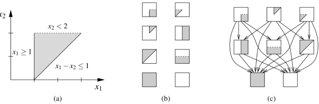
An example is given in Figure 1. The trianglex1≥1∧x2<2∧x1−x2≤1 inR2has three com-ponents of dimension 0 corresponding to its vertices(1,0)(in),(1,2)(out) and(3,2)(out), three com-ponents of dimension 1 associated to its sides (twoinand oneout), and two components of dimension 2 corresponding to its interior (in) and exterior (out) points.
3.3 Incidence Relation
In Section 3.1, we have established a link between the components of a polyhedron P⊆Rn and the
x2
x2<2
x1−x2≤1 x1≥1
x1
(a) (b) (c)
Figure 1: Example of (a) polyhedron, (b) polyhedral components, and (c) incidence relation.
between the SCC of an automaton: That a SCCS2is reachable from a SCCS1implies that every finite prefix that reaches a state ofS1can be followed by a suffix that ends up visitingS2, while the reciprocal property does not hold. In a similar way, we can define anincidence relationbetween the components of a polyhedron.
Definition 1 Let Q1,Q2be distinct components of a polyhedron P⊂Rn, with n∈N>0. The component Q2isincidentto Q1, denoted Q1≺Q2, iff for all~v1∈Rn such that P~v1 =Q1 andε ∈R>0, there exists
~v2∈Rnsuch that P~v2 =Q2and|~v1−~v2|<ε.
Remark that the incidence relation between the components of a polyhedron is a partial order, and thatQ1≺Q2 implies dim(Q1)<dim(Q2). As an example, in the triangle depicted in Figure 1, each side is incident to the vertices it links, since every neighborhood of a vertex contains points from its adjacent sides. The reverse property does not hold. The interior and exterior components of the triangle are incident to each of its sides and vertices.
3.4 How RVA Recognize Vectors
We are now able to explain the mechanism employed by a RVAA in order to check whether the vector
encoded by a word w belongs or not to a polyhedron P⊆Rn. After reading an integer part and a
separator symbol, the wordwfollows some transitions in the fractional part ofA, reaching a first
non-trivial strongly connected componentS1 (that is, a component containing at least one cycle). At this location inw, inserting arbitrary iterations of cycles withinS1would not affect the accepting status ofw. This intuitively means that the prefixwkofwread so far has led us to a point that belongs to a component
Q1 ofP, and that the decision can now be carried out further in an arbitrarily small neighborhood of this point. Reading additional symbols from w, one either stays within S1, or follows transitions that eventually lead to another non-trivial strongly connected componentS2. Once again, this means that the decision can now take place in an arbitrarily small neighborhood of a point belonging to a componentQ2 ofP, such that eitherQ1=Q2orQ1≺Q2. The same procedure repeats itself untilwreaches a strongly connected component that it does not leave anymore.
In other words, in order to decide whether to accept or not a word w, the RVA A first chooses
Let us now study more finely the mechanism used for moving from a componentQ1 that does not contain the vector~vto another componentQ2from which~v∈Pcan be decided. One follows a path of
A that leaves a strongly connected component associated toQ1, travels through an acyclic structure of
transitions, and finally reaches a SCC associated toQ2. Recall that, as discussed in Section 3.1, at each step in this path, the prefixwk ofwread so far determines an-cubeCwk. Thisn-cube covers some subset
Uwk ={P~u|~u∈Cwk}of the components ofP. IfUwk contains a single minimal component with respect
to the incidence order≺, then this component is necessarily equal toQ2, and its associated SCC is the only possible destination ofwk. Indeed, all components inUwkare then either equal or incident toQ2. If,
on the other hand,Uwk contains more than one minimal component, then further transitions have to be
followed in order to discriminate between them.
4
Implicit Real Vector Automata
Our goal is to define a data structure representing a polyhedron P⊆Rn that is more concise than a
RVA, but from which one can decide~v∈Pusing a similar procedure to the one outlined in Section 3.4. There are essentially three operations to consider: Selecting from a vector~van initial polyhedral com-ponent from which the decision can be started, checking whether~vbelongs or not to a given component, and moving from a component that does not contain~vto another one from which the decision can be continued. We study separately each of these problems in the three following sections.
4.1 Choosing an Initial Component
An easy way of managing the choice of an initial component is to consider only polyhedra in which this component is unique. This can be done without loss of generality thanks to the following definition.
Definition 2 Let P⊆Rnbe a polyhedron, with n∈N>0. Therepresenting coneof P is the polyhedron P⊆Rn+1={λ(x1, . . . ,xn,1)|λ∈R>0∧(x1, . . . ,xn)∈P}.
For every polyhedronP⊆Rn, the polyhedronPis conical inRn+1with respect to the apex~0, from
which it can be inferred that every neighborhood of~0 contains a unique minimal componentQ0 with respect to the incidence order≺. It follows that for every~v∈Rn+1, the decision~v∈Pcan be started from Q0. Remark thatPdescribesPwithout ambiguity, sincePcan be reconstructed fromPby computing its intersection with the constraintxn+1=1, and projecting the result over the firstnvector components. In the sequel, we assume w.l.o.g. that the polyhedra that we consider are conical with respect to the apex~0. A similar mechanism is employed in [19].
4.2 Deciding Membership in a Component
Consider a polyhedronP⊆Rnthat is conical with respect to the apex~0. As explained in Section 3.2, a
component of such a polyhedron is characterized by a vector space, a Boolean polarity (eitherinorout), and its incident components. Checking whether a given vector~v∈Rnbelongs or not to the component
reduces to deciding whether~vbelongs to its associated vector space. This is a simple algebraic operation if, for instance, the vector space is represented by a vector basis {~b1,~b2, . . . ,~bm}: One simply has to
check whether~vis linearly dependent with{~b1,~b2, . . . ,~bm}. This approach leads to a much more concise
4.3 Moving from a Component to Another
We now address the problem of leaving a componentQ1of a polyhedronP⊆Rn that does not contain a vector~v∈Rn, and moving to a componentQ2 that is incident to Q1, and from which~v∈P can be decided.
A first solution would be to borrow from a RVA representingPthe acyclic structure of transitions leaving the strongly connected componentsS1associated toQ1. However, this would negate the advan-tage in conciseness obtained in Section 4.2, since this acyclic structure of transitions is generally as large asS1itself.
The solution we propose consists in performing a variable change operation. Let {~y1,~y2, . . . ,~ym},
with 0<m≤n, be a basis of the vector space associated with the componentQ1. Ifm=n, thenQ1is universal and there is no possibility of leaving it. Ifm<n, then we introducen−madditional vectors
~z1,~z2, . . . ,~zn−m, such that{~y1, . . . ,~ym,~z1, . . . ,~zn−m}forms a basis ofRn. These additional vectors can be
chosen in a canonical way by selecting among(1,0, . . . ,0),(0,1, . . . ,0), . . . ,(0,0, . . . ,1), considered in that order,n−mvectors that are linearly independent with{~y1,~y2, . . . ,~ym}.
We then express the vector~vin the coordinate system{~y1, . . . ,~ym,~z1, . . . , ~zn−m}, obtaining a vector
(y1, . . . ,ym,z1, . . . ,zn−m). That~v leavesQ1 simply means that we have(z1, . . . ,zn−m)6=~0. As a
conse-quence, we associate Q1 with an acyclic structureD1 of outgoing transitions, recognizing prefixes of encodings of non-zero vectors(z1, . . . ,zn−m), in order to map these vectors to the polyhedral components
(incident toQ1) to which they lead.
A difficulty is that, from Theorem 2, the setPhas a conical structure in arbitrary small neighborhoods of points inQ1. If follows that the structureD1 has to map onto the same polyhedral component two
vectors~z and~z′ such that~z′ =λ~zfor someλ ∈R>0. An efficient solution is tonormalize the vectors
handled by D1: Given a vector~z= (z1, . . . ,zn−m) such that~z6=~0, we define its normalized form as [~z] = (1/(2.maxi|zi|))~z. In other words,[~z]is obtained by turning~zinto the half-line{λ~z|λ∈R>0}, and computing the intersection of this half-line with the faces of thenormalization cube[−1/2,1/2]n−m. In
this way, two vectors that only differ by a positive factor share the same normalized form, and will thus be handled identically.
The purpose of the structure D1 is thus to recognize normalized forms of vectors, and map them
onto the polyhedral components to which they lead. In order to define the transition graph of D1,
one therefore needs a suitable encoding for normalized forms of vectors. Using the standard posi-tional encoding of vectors in a base r∈N>1 is possible, but inefficient. We instead use the
follow-ing scheme. An encodfollow-ing of a normalized vector[~v] = ([v]1,[v]2. . . ,[v]n−m) starts with a leading
sym-bol a∈ {−1,+1,−2,+2, . . . ,−(n−m),+(n−m)} that identifies the face of the normalization cube [−1/2,1/2]n−m to which [~v] belongs: If a=−i, with 1≤i≤n−m, then [v]
i =−1/2; if a= +i,
then [v]i = +1/2. This prefix is followed by a suffix w∈ {0,1}ω that encodes the position of [~v]
within the face of the normalization cube defined by a. This suffix is obtained as follows. Assume that we havea∈ {−i,+i}, with 1≤i≤n−m (which implies [v]i∈ {−1/2,1/2}). We turn [~v] into
[[~v]] = ([v1], . . . ,[vi−1],[vi+1], . . . ,[vn−m]) + (1/2,1/2, . . . ,1/2), i.e., we remove the i-th vector
compo-nent, and offset the result in order to obtain[[~v]]∈[0,1]n−m−1. We then define w∈ {0,1}ω
as a word such that 0⋆wis a serialized binary encoding of[[~v]]. Note that some vectors~vmay belong to several faces of the normalization cube, hence their normalized form may admit multiple encodings. This is not problematic, provided that the structureD1handles these encodings consistently.
In summary, the structure D1 is an acyclic decision graph that partitions the space of normalized
vectors according to their destination components. Each prefixwkof lengthkread byD1corresponds to a convex regionRwk ⊂R
nthat is conical in every neighborhood of any element ofQ
as apex. The situation is similar to that discussed in Section 3.4: If in a sufficiently small neighborhood of any point ofQ1, the set of components ofPcovered byRwkcontains a unique minimal componentQ2
with respect to the incidence order≺, thenwk leads toQ2. Otherwise, the decision process is not yet complete, and additional transitions have to be followed inD1.
4.4 Data Structure
We are now ready to describe our proposed data structure for representing arbitrary polyhedra of Rn,
with n∈N>0. Recall that we assume w.l.o.g. that the polyhedra we consider are conical in Rn with
respect to the apex~0.
4.4.1 Syntax
Definition 3 AnImplicit Real Vector Automaton (IRVA)is a tuple(n,SI,SE,s0,∆), where
• n is adimension.
• SI is a set of implicit states. Each s∈SI is associated with a vector spaceVS(s)⊆Rn, and a
Booleanpolaritypol(s)∈ {in,out}.
• SE is a set of explicit states, such that SE ∩SI=/0.
• s0∈SI is theinitial state.
• ∆:SI× ±N>0 ∪ SE× {0,1} →(SI∪SE)is a (partial)transition relation.
In order to be well formed, an IRVA(n,SI,SE,s0,∆)representing a polyhedronP⊆Rnhas to satisfy some integrity constraints. In particular, the transition relation∆must be acyclic, and for alls1,s2∈SI
such that∆directly or transitively leads froms1 tos2, one must have VS(s1)⊂VS(s2). The transition relation∆is required to be complete, in the sense that, for every implicit states∈SIandi∈N>0,∆(s,+i) and∆(s,−i)are defined iffi≤n−dim(VS(s)). Furthermore, for every explicit states∈SE, both∆(s,0)
and∆(s,1)must be defined. Finally, each component of Pmust be described by a state inSI, and for
every pairQ1,Q2of components ofPsuch thatQ1≺Q2, there must exist a sequence of transitions in∆ leading from the implicit state associated toQ1to the one associated toQ2. In other words, the order≺ between the components ofPcan straightforwardly be recovered from the reachability relation between the implicit states representing them.
4.4.2 Semantics
The semantics of IRVA is defined by the following procedure, that decides whether a given vector~v∈Rn
belongs or not to the polyhedron P represented by an IRVA (n,SI,SE,s0,∆). The principles of this procedure have already been outlined in Sections 4.2 and 4.3.
One starts at the implicit states0. At each visited implicit states, one first decides whether~v∈VS(s). In case of a positive answer, the procedure concludes that~v∈Pif pol(s) =in, and that~v6∈Potherwise. In the negative case, the decision has to be carried out further. The vector~vis transformed into~v′according to the variable change operation associated to VS(s). Then,~v′is normalized into a vector[~v′], which is encoded into a wordw∈ ±N{0,1}ω. (In the case of multiple encodings, one of them can arbitrarily be
4.4.3 Examples
An IRVA representing the setx1≥1∧x2<2∧x1−x2≤1 inR2, considered in Figure 1(a), is given in Figure 2. Note that, since the set is not conical, the IRVA actually recognizes its representing cone, as discussed in Section 4.1. In this figure, implicit states are depicted by rounded boxes, and explicit ones by small circles. Doubled boxes representinpolarities. The vector spaces associated to implicit states are represented by one of their bases. Remark that the layout of the implicit states and the decision structures linking them closely matches the polyhedral components and their incidence relation as depicted in Figure 1(c), except for the initial state which corresponds to the apex~0 of the representing cone.
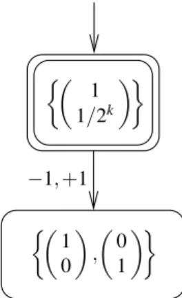
As an additional example, Figure 3 shows how the setx1=2kx2inR2, discussed in the introduction of Section 3, is represented by an IRVA. In this case, the gain in conciseness is exponential with respect to RVA.
5
Manipulation Algorithms
5.1 Test of Membership
A procedure for checking whether a given vector belongs to a polyhedron represented by an IRVA has already been outlined in Section 4.4.2. In the case of a polyhedron P⊆Rn that is not conical, an
IRVA can be obtained for its representing cone P⊂Rn+1, as discussed in Section 4.1. In this case,
checking whether a vector (v1,v2, . . . ,vn) ∈Rn belongs to P simply reduces to determining whether
(v1,v2, . . . ,vn,1)belongs toP, which is done by the algorithm of Section 4.4.2.
5.2 Minimization
An IRVA(n,SI,SE,s0,∆)can be minimized in order to reduce its number of implicit and explicit states. Since the transition relation∆is acyclic, the explicit and implicit states can be processed in a bottom-up order, starting from the implicit states with the largest vector spaces. At each step, reduction rules are applied in order simplify the current structure. A first rule is aimed at merging states that are indis-tinguishable: If two explicit states share the same successors, they can be merged. In the case of two implicit states, one additionally has to check that their associated vector spaces are equal, and that their polarities match. The purpose of the second rule is to get rid of unnecessary decisions. Consider a state s(either implicit or explicit) with an outgoing transition that leads to an implicit states1, representing a polyhedron componentQ1. If all the implicit statessi that are reachable fromsare also reachable from
s1, then these implicit states represent polyhedral componentsQi such that eitherQi=Q1orQ1≺Qi.
The statescan then be absorbed intos1, provided thatsis not an implicit state with a different polarity from the one ofs1. Note that this reduction rule correctly handles the case of a statesthat is implicit and does not correspond to a polyhedral component, but to a proper subset of the componentQ1represented bys1. For example, inR2,smay correspond to a unidimensional linex1−x2=0 covered by the larger
universal componentR2represented bys1.
Property 1 Minimized IRVA are canonical up to isomorphism of their transition relation, and equality
of the vector spaces associated to their implicit states.
Proof sketch:The canonicity of a minimized IRVAA representing a polyhedronP⊆Rn is the
1 2 1 1 0 1 1 2/3 1/3
1 0 1 , 0 1 −1 1 0 0 , 0 1 1/2
1 0 1 , 0 1 0 1 0 0 , 0 1 0 , 0 0 1 1 0 0 , 0 1 0 , 0 0 1 +2 +1 +3
−1,−2,−3
1 0 0 1 0 1 0 1 0 1 0 1 0 1 0 0 1 1 0 1 0 1 −2
−1,+2 +1
+2 +1
−1,−2
−1
+1,+2
−2
+1 +1
−1 −1
−1 +1
1 1/2k
1 0
,
0 1
−1,+1
Figure 3: IRVA representing the set{(x1,x2)∈R2|x1=2kx2}.
do not represent such components. This yields a one-to-one relationship between the implicit states of
A and the polyhedral components ofP. Second, the transition structure leaving an explicit statesofA
satisfies the following constraints. As discussed in Section 4.3, the statescorresponds to a component QofP, and every prefixwk of lengthk read fromsdefines a convex conical region Rs,wk ⊂R
n. If, in
all sufficiently small neighborhoods ofQ, the region Rs,wk covers a unique componentQ
′ ofPthat is
minimal with respect to the incidence order, then the path readingwkfromsleads to the implicit states′
corresponding toQ′. Provided that explicit states that have identical successors are merged, this property characterizes precisely the decision structure leavings. Such structures will then be isomorphic in all
minimized IRVA representing the same polyhedron.
5.3 Boolean Combinations
In order to apply a Boolean operator to two polyhedraP1andP2 respectively represented by IRVAA1 andA2, one builds an IRVAA that simulates the concurrent behavior ofA1 andA2. The procedure is
analogous to the computation of the product of two finite-state automata. The initial implicit state ofA
is obtained by combining the initial states ofA1andA2, which amounts to intersecting their associated
vector spaces, and applying the appropriate Boolean operator to their polarities. Each time an implicit statesis added toA, representing a polyhedron componentQ, its successors are recursively explored.
As explained in Section 4.3, each finite prefixwk, of lengthk, read fromscorresponds to a convex conical
regionRs,wk⊂R
n. The idea is to check, in a sufficiently small neighborhoodRofQ, whetherR
s,wkcovers
unique minimal componentsQ1ofP1andQ2ofP2, with respect to their respective incidence orders. In the positive case, one computes the intersection of the underlying vector spaces ofQ1 andQ2. If the resulting vector space has a higher dimension than dim(VS(s)), as well as a non-empty intersection with Rs,wk, a corresponding new implicit state is added toA. In all other cases, the decision structure leaving
shas to be further developed, which amounts to creating new explicit states and new transitions between them, in order to read prefixes longer thanwk.
A key operation in the previous procedure is thus to compute, from an IRVA representing a polyhe-dronP, a componentQofP, and a given convex conical regionC, the unique minimal component ofP (if it exists) covered byCin the neighborhood ofQ, with respect to the incidence order≺. This is done by exploring the IRVA starting from the implicit state representingQ. From a given implicit states, the exploration only has to consider the paths labeled by wordswksuch thatC∩Rs,wk 6=/0, until they reach
checks whether its underlying vector space has a non-empty intersection withC. If this check succeeds for some nonempty subset ofS, then the procedure returns its minimal component, or fails when such a component does not exist. Otherwise, it can be shown that the exploration can be continued from a sin-gle state chosen arbitrarily inS. The regions of space that are manipulated by this procedure are convex polyhedra, and can be handled by specific data structures [3].
6
Conclusions
We have introduced a data structure, the Implicit Real Vector Automaton (IRVA), that is expressive enough for representing arbitrary polyhedra inRn, closed under Boolean operators, and reducible to a
canonical form up to isomorphism.
IRVA share some similarities with the data structure described in [14], which also relies on decom-posing polyhedra into their components, and representing the incidence relation between them. The main original feature of our work is the decision structures that link each component to its incident ones, which are not limited to three spatial dimensions, and lead to a canonical representation. Furthermore, by imi-tating the behavior of RVA, we have managed to obtain a symbolic representation of polyhedra in which the membership of a vector can be decided by following a single automaton path, which is substantially more efficient that the procedure proposed in [14].
The algorithms sketched in Section 5 are clearly polynomial. We have not yet precisely studied their worst-case complexity, since they depend on manipulations of convex polyhedra, the practical cost of which is expected to be significantly lower than their worst-case one. In order to assess the cost of building and handling IRVA in actual applications, a prototype implementation of those algorithms is under way. The example given in Figure 2 has been produced by this prototype.
Future work will address other useful operations such as projection of polyhedra, conversions to and from other representations, and operations that are specific to symbolic state-space exploration al-gorithms. For this particular application, IRVA in their present form are still impractical, since they only provide efficient representations of polyhedra in spaces of small dimension. (Indeed, the size of an IRVA grows with the number of components of the polyhedron it represents, and simple polyhedra such asn-cubes have exponentially many components in the spatial dimensionn.) We plan on tackling this problem by applying to IRVA the reduction techniques proposed in [4], which seems feasible thanks to the acyclicity of their transition relation. This would improve substantially the efficiency of the data structure for large spatial dimensions.
Acknowledgement
We wish to thank J´erˆome Leroux for fruitful technical discussions about the data structure presented in this paper.
References
[1] R. Alur, C. Courcoubetis, N. Halbwachs, T. A. Henzinger, P.-H. Ho, X. Nicollin, A. Olivero, J. Sifakis & S. Yovine (1995): The Algorithmic Analysis of Hybrid Systems. Theoretical Computer Science 138, pp. 3–34.
[2] R. Alur, T. A. Henzinger & P.-H. Ho (1993): Automatic Symbolic Verification of Embedded Systems. In:
[3] R. Bagnara, E. Ricci, E. Zaffanella & P. M. Hill (2002): Possibly Not Closed Convex Polyhedra and the Parma Polyhedra Library. In:Proc. 9th SAS,LNCS2477, Springer-Verlag, London, pp. 213–229.
[4] V. Bertacco & M. Damiani (1997):The disjunctive decomposition of logic functions. In:Proc. ICCAD, IEEE Computer Society, pp. 78–82.
[5] B. Boigelot (1998):Symbolic Methods for Exploring Infinite State Spaces. Ph.D. thesis, Universit´e de Li`ege. [6] B. Boigelot, L. Bronne & S. Rassart (1997):An Improved Reachability Analysis Method for Strongly Linear
Hybrid Systems. In:Proc. 9th CAV,LNCS1254, Springer, Haifa, pp. 167–177.
[7] B. Boigelot, J. Brusten & J. Leroux (2009):A Generalization of Semenov’s Theorem to Automata over Real Numbers. In:Proc. 22nd CADE,LNCS5663, Springer, Montreal, pp. 469–484.
[8] B. Boigelot, S. Jodogne & P. Wolper (2005):An Effective Decision Procedure for Linear Arithmetic over the Integers and Reals.ACM Transactions on Computational Logic6(3), pp. 614–633.
[9] B. Boigelot, S. Rassart & P. Wolper (1998):On the Expressiveness of Real and Integer Arithmetic Automata. In:Proc. 25th ICALP,LNCS1443, Springer, Aalborg, pp. 152–163.
[10] P. Cousot & N. Halbwachs (1978):Automatic discovery of linear restraints among variables of a program. In:Conf. rec. 5th POPL, ACM Press, New York, pp. 84–96.
[11] D. L. Dill (1989):Timing assumptions and verification of finite-state concurrent systems. In:Prof. of Auto-matic Verification Methods for Finite-State Systems, number 407 in LNCS, Springer-Verlag, pp. 197–212. [12] J. Ferrante & C. Rackoff (1975): A Decision Procedure for the First Order Theory of Real Addition with
Order.SIAM Journal on Computing4(1), pp. 69–76.
[13] J. E. Goodman & J. O’Rourke, editors (2004): Handbook of discrete and computational geometry. CRC Press LLC, Boca Raton, 2nd edition.
[14] M. Granados, P. Hachenberger, S. Hert, L. Kettner, K. Mehlhorn & M. Seel (2003):Boolean Operations on 3D Selective Nef Complexes – Data Structure, Algorithms, and Implementation. In:Proc. 11th ESA,LNCS
2832, Springer, pp. 654–666.
[15] N. Halbwachs, P. Raymond & Y.E. Proy (1994):Verification of Linear Hybrid Systems By Means of Convex Approximations. In:Proc. 1st SAS,LNCS864, Springer-Verlag, pp. 223–237.
[16] T. A. Henzinger (1996): The Theory of Hybrid Automata. In: Proc. 11th LICS, IEEE Computer Society Press, pp. 278–292.
[17] T. A. Henzinger & P.-H. Ho (1994): Model Checking Strategies for Linear Hybrid Systems (Extended Ab-stract). In:Proc. of Workshop on Formalisms for Representing and Reasoning about Time.
[18] The Li`ege Automata-based Symbolic Handler (LASH). Available at : http://www.montefiore.ulg.ac. be/~boigelot/research/lash/.
[19] H. Le Verge (1992):A note on Chernikova’s Algorithm. Technical Report, IRISA, Rennes.
[20] Linear Integer/Real Arithmetic solver (LIRA). Available at :http://lira.gforge.avacs.org/.
[21] C. L¨oding (2001):Efficient Minimization of Deterministic Weakω-Automata.Information Processing Letters
79(3), pp. 105–109.
[22] T. S. Motzkin, H. Raiffa, G. L. Thompson & R. M. Thrall (1953): The Double Description Method. In:
Contributions to the Theory of Games – Volume II, number 28 in Annals of Mathematics Studies, Princeton University Press, pp. 51–73.
[23] F. Rossi, P. van Beek & T. Walsh, editors (2006):Handbook of constraint programming. Elsevier. [24] A. Schrijver (1986):Theory of linear and integer programming. John Wiley & Sons, Inc., New York. [25] M. Vardi (2007):The B¨uchi Complementation Saga. In:Proc. 24th. STACS,LNCS4393, Springer, Aachen,
pp. 12–22.