Expressiveness modulo Bisimilarity of Regular Expressions with Parallel Composition (Extended Abstract)

S. Fr¨oschle, F.D. Valencia (Eds.): Workshop on Expressiveness in Concurrency 2010 (EXPRESS’10). EPTCS 41, 2010, pp. 1–15, doi:10.4204/EPTCS.41.1

with Parallel Composition

(Extended Abstract)

Jos C. M. Baeten

Eindhoven University of Technology, The Netherlands [email protected]

Bas Luttik

Eindhoven University of Technology, The Netherlands Vrije Universiteit Amsterdam, The Netherlands

[email protected] Tim Muller

University of Luxembourg, Luxembourg [email protected]

Paul van Tilburg

Eindhoven University of Technology, The Netherlands [email protected]

The languages accepted by finite automata are precisely the languages denoted by regular sions. In contrast, finite automata may exhibit behaviours that cannot be described by regular expres-sions up to bisimilarity. In this paper, we consider extenexpres-sions of the theory of regular expresexpres-sions with various forms of parallel composition and study the effect on expressiveness. First we prove that adding pure interleaving to the theory of regular expressions strictly increases its expressiveness modulo bisimilarity. Then, we prove that replacing the operation for pure interleaving by ACP-style parallel composition gives a further increase in expressiveness. Finally, we prove that the theory of regular expressions with ACP-style parallel composition and encapsulation is expressive enough to express all finite automata modulo bisimilarity. Our results extend the expressiveness results ob-tained by Bergstra, Bethke and Ponse for process algebras with (the binary variant of) Kleene’s star operation.

1

Introduction

A well-known theorem by Kleene states that the languages accepted by finite automata are precisely the languages denoted by a regular expression (see, e.g., [8]). Milner, in [10], showed how regular expres-sions can be used to describebehaviour by defining an interpretation of regular expressions directly as finite automata. He then observed that the process-theoretic counterpart of Kleene’s theorem —stating that every finite automaton is described by a regular expression— fails: there exist finite automata whose behaviours cannot faithfully, i.e., up to bisimilarity, be described by regular expressions. Baeten, Corra-dini and Grabmayer [1] recently found a structural property on finite automata that characterises those that are denoted with a regular expression modulo bisimilarity. In this paper, we study to what extent the expressiveness of regular expressions increases when various forms of parallel composition are added.

Our first contribution, in Section 3, is to show that adding an operation for pure interleaving to regular expressions strictly increases their expressiveness modulo bisimilarity. A crucial step in our proof consists of characterising the strongly connected components in finite automata denoted by regular expressions. The characterisation allows us to prove a property pertaining to the exit transitions from such strongly connected components. If interleaving is added, then it is possible to denote finite automata violating this property.

between components, leads to a further increase in expressiveness. To this end, we first characterise the strongly connected components in finite automata denoted by regular expressions with interleaving, and deduce a property on the exit transitions from such strongly connected components. Then, we present an expression in the theory of regular expressions with ACP-style parallel composition that denotes a finite automaton violating this property.

Our third contribution, in Section 5, is to establish that adding ACP-style parallel composition and encapsulation to the theory of regular expressions actually yields a theory in which every finite automaton can be expressed up to isomorphism, and hence, since bisimilarity is coarser than isomorphism, also up to bisimilarity. Every expression in the resulting theory, in turn, denotes a finite automaton, so this result can be thought of as an alternative process-theoretic counterpart of Kleene’s theorem.

The results in this paper are inspired by the results of Bergstra, Bethke and Ponse pertaining to the relative expressiveness of process algebras with a binary variant of Kleene’s star operation. In [3] they establish an expressiveness hierarchy on the extensions of the process theories BPA(A_{), BPAδ(}A_), PA(A_{), PAδ(}A_{), ACP(}A_,γ_{), and ACPτ(}A_,γ_{)with binary Kleene star. The reason that their results are} based on extensions with the binary version of the Kleene star is that they want to avoid the process-theoretic complications arising from the notion of intermediate termination (we say that a state in a finite automaton is intermediately terminating if it is terminating but also admits a transition). Most of the expressiveness results in [3] are included in [4], with more elaborate proofs.

Casting our contributions mentioned above in process-theoretic terminology, we establish a strict expressiveness hierarchy on the process theories BPA∗_0,1(A_{) (regular expressions) modulo bisimilarity,} PA∗_0,1(A_{)(regular expressions with interleaving) modulo bisimilarity and ACP}∗

0,1(A,γ)(regular expres-sions with ACP-style parallel composition and encapsulation) modulo bisimilarity. The differences be-tween the process theories BPA_δ(A_{), PAδ(}A_{)and ACP(}A_,γ_{)considered [3, 4] and the process theories} BPA∗_0,1(A_{), PA}∗

0,1(A)and ACP∗0,1(A,γ)considered in this paper are as follows: we write0for the con-stant deadlock which is denoted byδ in [3, 4], we include the unary Kleene star instead of its binary variant, and we include a constant1denoting the successfully terminated process. The first difference is, of course, cosmetic, and with the addition of the constant1the unary and binary variants of Kleene’s star are interdefinable. So, our results pertaining to the relative expressiveness of BPA∗_0,1(A_{), PA}∗

0,1(A) and ACP∗_0,1(A_,γ_{)extend the expressiveness hierarchy of [3, 4] with the constant}1.

In [4] the expressiveness proofs are based on identifying cycles and exit transitions from these cycles. There are two reasons why the proofs in [3] and [4] cannot easily be adapted to a setting with1. First, in a setting with1and Kleene star there are cycles without any exit transitions. Second, the inclusion of the empty process1gives intermediate termination, which, combined with the previously described different behaviour of cycles, forces us to consider the more general structure of strongly connected component.

2

Preliminaries

In this section, we present the relevant definitions for the process theory ACP∗_0,1(A,γ) and its subthe-ories PA∗_0,1(A_{) and BPA}∗

0,1(A). We give their syntax and operational semantics, and the notion of (strong) bisimilarity. We also introduce some auxiliary technical notions that we need in the remain-der of the paper, most notably that of strongly connected component. The expressions of the process theory BPA∗_0,1(A_{) are precisely the well-known regular expressions from the theory of automata and} formal languages, but we shall consider the automata associated with them modulo bisimilarity instead of modulo language equivalence.

commu-nication functionγ onA_{, i.e., an associative and commutative binary partial operation}γ _:A_×A_⇀A_. ACP∗_0,1(A_,γ_{)incorporates a form of synchronisation between the components of a parallel composition} by allowing certain actions to engage in acommunicationresulting in another action. The communica-tion funccommunica-tionγ then defines which actions may communicate and what is the result. The details of this feature will become clear when we present the operational semantics of parallel composition.

The set of ACP∗_0,1(A_,γ_)expressionsP_ACP∗

0,1(A,γ)is generated by the following grammar:

p::= 0 | 1 | a | p·p | p+p | p∗ | pkp | ∂H(p) ,

witharanging overA_{andHranging over subsets of}A_.

The process theory ACP(A_,γ_{) (excluding the constants 0 and 1, but including a constant} δ _with exactly the same behaviour as 0, and without the operation ∗) originates with [5]. The extension of ACP(A_,γ_{) with a constant1 was investigated by [9, 2, 14] (in these articles, the constant was denoted}

ε). The extension of ACP(A_,γ_{)with the binary version of the Kleene star was first proposed in [3]. The} reader already familiar with the process theory ACP∗_0,1(A,γ)will have noticed that the operationsT(left merge) and|(communication merge) are missing from our syntax definition. In [5], these operations are included as auxiliary operations necessary for a finite axiomatisation of the theory. They do not, however, add expressiveness in our setting with Kleene star instead of a general form of recursion. We have omitted them to achieve a more efficient presentation of our results.

The constants0and1respectively stand for the deadlocked process and the successfully terminated process, and the constantsa∈A_{denote processes of which the only behaviour is to execute the action} a. An expression of the form p·q is called asequential composition, an expression of the form p+q is called analternative composition, and an expression of the form p∗ is called a star expression. An expression of the form pkq is called aparallel composition, and an expression of the form ∂H(p) is called anencapsulation.

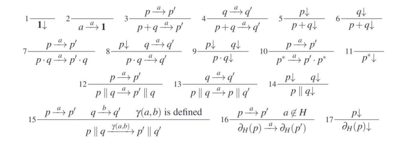
From the names for the constructions in the syntax of ACP∗_0,1(A_,γ_{), the reader probably has already} an intuitive understanding of the behaviour of the corresponding processes. We proceed to formalise the operational behaviour by means of a collection of operational rules (see Table 1) in the style of Plotkin’s Structural Operational Semantics [13]. Note how the communication function in rule 14 is employed to model a form of communication between parallel components: if one of the components of a parallel composition can execute a transition labelled with a, the other can execute a transition labelled withb, and the communication function γis defined onaand b, then the parallel composition can execute a transition labelled withγ(a,b). (It may help to think of the actionaas standing for the

event of sending some datumd, the actionbas standing for the event of receiving datumd, and the action

γ(a,b)as standing for the event that two components communicate datumd.) TheA_{-labelled transition} relation→ACP∗_0,1(A,γ)and the termination relation↓ACP∗_0,1(A,γ)onPACP∗_0,1(A,γ)are the least relations→ ⊆

P_ACP∗

0,1(A,γ)×

A_×P_ACP∗

0,1(A,γ)and↓ ⊆

P_ACP∗

0,1(A,γ)satisfying the rules in Table 1.

The triple T_ACP∗

0,1(A,γ)= (

P_ACP∗

0,1(A,γ),→ACP∗0,1(A,γ),↓ACP∗0,1(A,γ)), consisting of the ACP

∗

0,1(A,γ) ex-pressions together with theA_{-labelled transition relation and the termination predicate associated with} them, is an example of anA_{-labelled transition system space. In general, an}A_{-labelled transition system} space(S,→,↓)consists of a (non-empty) set S, the elements of which are calledstates, together with an A_{-labelled transition relation → ⊆S×}A_{×S and a subset ↓ ⊆S. We shall in this paper consider} two more examples of transition system spaces, obtained by restricting the syntax of ACP∗_0,1(A_,γ_)and making special assumptions about the communication function.

Next, we define the A_{-labelled transition system space} T_PA∗

0,1(A)= (PPA∗0,1(A),→PA∗0,1(A),↓PA∗0,1(A))

corresponding with the process theory PA∗_0,1(A_{). The set of PA}∗

1

1↓ 2 _a a −→1

3 p

a −→p′

p+q−→a p′ 4

q−→a q′

p+q−→a q′ 5 p↓

p+q↓ 6 q↓ p+q↓

7 p

a −→p′

p·q−→a p′·q

8 p↓ q

a −→q′

p·q−→a q′

9 p↓ q↓

p·q↓ 10

p−→a p′

p∗−→a p′·p∗

11

p∗↓

12 p

a −→p′

pkq−→a p′kq 13

q−→a q′

pkq−→a pkq′ 14

p↓ q↓ pkq↓

15 p

a

−→p′ q−→b q′ γ(a,b)is defined

pkq−−−−→γ(a,b) p′kq′

16 p

a

−→p′ a6∈H ∂H(p)−→a ∂H(p′) 17

p↓

∂H(p)↓

Table 1: Operational rules for ACP∗_0,1(A,γ), witha∈A_andH⊆A_.

the ACP∗_0,1(A_,γ_{)process expressions without occurrences of the construct}∂_{H( ). The PA}∗

0,1(A) transi-tion relatransi-tion→_PA∗

0,1(A)on

P_PA∗

0,1(A)and the termination predicate↓PA∗0,1(A)on

P_PA∗

0,1(A)are the transition

relation and termination predicate induced on PA∗_0,1(A_{) expressions by the operational rules in Table 1} minus the rules 15–17. Alternatively (and equivalently) the transition relation→PA∗_0,1(A₎can be defined

as the restriction of the transition relation→ACP∗_0,1(A,/0), with /0 denoting the communication function that

is everywhere undefined, toP_PA∗

0,1(A).

To define theA_{-labelled transition system space}T_BPA∗

0,1(A)= (PBPA∗0,1(A),→BPA∗0,1(A),↓BPA∗0,1(A))

as-sociated with the process theory BPA∗_0,1(A_{), let}P_BPA∗

0,1(A) consist of all PA

∗

0,1(A) expressions without occurrences of the construct k . The BPA∗_0,1(A_{)transition relation→BPA}∗

0,1(A)and the BPA

∗

0,1(A) termi-nation predicate↓_BPA∗

0,1(A)are the transition relation and the termination predicate induced on BPA

∗ 0,1(A) expressions by the operational rules in Table 1 minus the rules 12–17. That is,→BPA∗_0,1(A)and↓BPA∗_0,1(A)

are obtained by restricting→ACP∗_0,1(A,γ)and↓ACP∗_0,1(A,γ)toPBPA∗_0,1(A₎.

Henceforth, we shall omit the subscripts ACP∗_0,1(A_,γ_{), PA}∗

0,1(A) and BPA∗0,1(A) from transition relations and termination predicates whenever it is clear from the context which transition relation or termination predicate is meant. Furthermore, we shall often use ACP∗_0,1(A_,γ_{), PA}∗

0,1(A)and BPA∗0,1(A), respectively, to denote the associated transition system spacesT_ACP∗

0,1(A,γ),

T_PA∗

0,1(A)and

T_BPA∗

0,1(A).

LetT_{= (S,→,↓)be an}A_{-labelled transition system space. Ifs,s}′_{∈S, then we writes−→s}′_{if there} existsa∈A_{such thats−→}a _s′_{, ands 6−→s}′_{if there exists no sucha∈}A_{. We denote by→}+_{the transitive} closure of→, and by→∗the reflexive-transitive closure of→. Ifs−→∗s′then we say thats′isreachable froms; the set of all states reachable fromsis denoted by[s]→. We say that a statesisnormedif there existss′such thats−→∗_s′_ands′_{↓.Tis calledregularif[s]}

→is finite for alls∈S.

Lemma 2.1. The transition system spaces ACP∗_0,1(A_,γ_{), PA}∗

0,1(A), and BPA∗0,1(A)are all regular. With every state s inT _{we can associate an automaton(or: transition system) ([s]→},→ ∩([s]→× A_{×[s]→),↓ ∩[s]→, s). Its states are the states reachable froms, its transition relation and termination} predicate are obtained by restricting→and↓accordingly, and the statesis declared as theinitial stateof the automaton. If a transition system space is regular, then the automaton associated with a state in it is finite, i.e., it is a finite automaton in the terminology of automata theory. Thus, we get by Lemma 2.1 that the operational semantics of ACP∗_0,1(A_,γ_{), and, a fortiori, that of PA}∗

In automata theory, automata are usually considered as language acceptors and two automata are deemed indistinguishable if they accept the same languages. Language equivalence is, however, arguably too coarse in process theory, where the prevalent notion is bisimilarity [11, 12].

Definition 2.2. LetT_{1= (S1,→1,↓1)and}T_{2= (S2,→2,↓2)be transition system spaces. A binary relation} R_{⊆S1×S2is abisimulationbetween}T_1andT_{2if it satisfies, for alla∈}A_{and for alls1∈S1ands2∈S2} such thats1Rs2, the following conditions:

(i) if there existss′₁∈S1such thats1−→a 1s′1, then there existss′2∈S2such thats2−→a 2s2′ ands′1Rs′2;

(ii) if there existss′₂∈S2such thats2−→a 2s′2, then there existss′1∈S1such thats1−→a 1s1′ ands′1Rs′2;

and

(iii) s1↓1if, and only if,s2↓2.

Statess1∈S1and s2∈S2 arebisimilar (notation: s1↔s2) if there exists a bisimulationR betweenT1

andT_{2such thats1}R_s2.

To achieve a sufficient level of generality, we have defined bisimilarity as a relation between tran-sition system spaces; to obtain a suitable notion of bisimulation between automata one should add the requirement that the initial states of the automata be related.

Based on the associated transition system spaces, we can now define what we mean when some transition system space is, modulo bisimilarity, less expressive than some other transition system space.

Definition 2.3. Let T_{1 and} T_{2 be transition system spaces. We say that} T_{1 is less expressive than} T₂ (notation: T_1≺T_{2) if every state in}T_{1is bisimilar to a state in}T_{2, and, moreover, there is a state in}T₂ that isnotbisimilar to some state inT_1.

When we investigate the expressiveness of ACP∗_0,1(A_,γ_{), we want to be able to choose} γ_{. So,} we are actually interested in the expressiveness of the (disjoint) union of all transition system spaces ACP∗_0,1(A_,γ_)withγ _{ranging over all communication functions. We denote this transition system space} byS

γACP∗0,1(A,γ). In this paper we shall then establish that BPA∗0,1(A)≺PA∗0,1(A)≺

S

γACP∗0,1(A,γ). We recall below the notion of strongly connected component (see, e.g., [6]) that will play an impor-tant rˆole in establishing that the above hierarchy of transition system spaces is strict.

Definition 2.4. Astrongly connected componentin a transition system spaceT_{= (S,→,↓)is a maximal} subsetCofSsuch thats−→∗s′for alls,s′∈C. A strongly connected componentCistrivialif it consists of only one state, sayC={s}, ands 6−→s; otherwise, it isnon-trivial.

Note that every element of a transition system space is an element of precisely one strongly connected component of that space. Furthermore, ifsis an element of a non-trivial strongly connected component, then s−→+_{s. Since in a strongly connected component from every element every other element can}

be reached, we get as a corollary to Lemma 2.1 that strongly connected components in ACP∗_0,1(A_,γ_), PA∗_0,1(A_{)and BPA}∗

0,1(A)are finite.

Let T_{= (S,→,↓) be a transition system space, let s∈S, and let C⊆S be a strongly connected} component inS. We say thatCisreachablefromsifs−→∗s′for alls′∈C.

Lemma 2.5. LetT_{1= (S1,→1,↓1) and} T_{2 = (S2,→2,↓2)be regular transition system spaces, and let} s1∈S1 and s2∈S2 be such thats1↔s2. Ifs1 is an element of a strongly connected componentC1in

T_{1, then there exists a strongly connected componentC2reachable froms2satisfying that for alls}′

1∈C1

3

Relative Expressiveness of

BPA

(

A

₎

_and

_PA

(

A

)

In [3] it is proved that BPA∗₀(A_{) is less expressive than PA}∗

0(A). The proof in [3] is by arguing that the PA∗₀(A_{) expression(a·b)}∗_{ckdis not bisimilar with a BPA}∗

0(A)expression. (Actually, the PA∗0(A) expression employed in [4] uses only a single actiona, i.e., considers the PA∗₀(A_{)expression(a·a)}∗_ak a; we use the actions b, c and d for clarity.) An alternative and more general proof that the PA∗₀(A₎ expression above is not expressible in BPA∗₀(A_{)is presented in [4]. There it is established that the PA}∗

0(A) expression above fails the following general property, which is satisfied by all BPA∗₀(A_{)-expressible} automata:

IfCis a cycle in an automaton associated with a BPA∗₀(A_{)expression, then there is at most} one state p∈Cthat has an exit transition.

(A cycle is a sequence(p1, . . . ,pn)such that pi−→pi+1(1≤i<n) andpn−→p1; an exit transition from

piis a transition pi−→p′isuch that no element of the cycle is reachable fromp′i.)

The following example shows that automata associated with BPA∗_0,1(A_{) expressions do not satisfy} the property above.

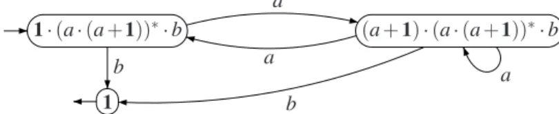
Example 3.1. Consider the automaton associated with the BPA∗_0,1(A_{)expression1·(a·(a+1))}∗_·b(see Figure 1) with a cycle; both states on the cycle have ab-transition off the cycle.

1·(a·(a+1))∗·b (a+1)·(a·(a+1))∗·b

1

a

b a _a

b

Figure 1: A transition system in BPA∗_0,1(A_{)with a cycle with multiple exit transitions.}

In this section we shall establish that BPA∗_0,1(A_{) is less expressive than PA}∗

0,1(A). As in [4] we prove that BPA∗_0,1(A_{)-expressible automata satisfy a general property that some automaton expressible} in PA∗_0,1(A_{)fails to satisfy. We find it technically convenient, however, to base our relative expressiveness} proofs on the notion of strongly connected component, instead of cycle. Note, e.g., that every process expression is an element of precisely one strongly connected component, while it may reside in more than one cycle. Furthermore, ifp−→qand pandqare in distinct strongly connected components, then we can be sure thatp−→qis an exit transition, while ifpandqare on distinct cycles, then it may happen that pis reachable fromq.

3.1 Strongly Connected Components inBPA∗_0,1(A₎

We shall now establish that a non-trivial strongly connected component in BPA∗_0,1(A_{) is either of the} form{p1·q∗, . . . ,pn·q∗}withpi(0≤i≤n) reachable fromqand{p1, . . . ,pn}not a strongly connected

component, or of the form {p1·q, . . . ,pn·q} where {p1, . . . ,pn} is a strongly connected component. To this end, let us first establish, by reasoning on the basis of the operational semantics, that process expressions in a non-trivial strongly connected component are necessarily sequential compositions; at the heart of the argument will be the following measure on process expressions.

(i) #(0) =#(1) =0, and #(a) =1;

(ii) #(p·q) =0 ifqis a star expression, and #(p·q) =#(q) +1 otherwise;

(iii) #(p+q) =max{#(p),#(q)}+1; and (iv) #(p∗) =1.

We establish that #( )is non-increasing over transitions, and, in fact, in most cases decreases.

Lemma 3.3. Ifpand p′are BPA∗_0,1(A_{)expressions such that p−→}+_p′_{, then #(p)≥#(p}′_{). Moreover, if} #(p) =#(p′), then p=p1·qand p′=p′1·qfor some p1, p′1andq.

Proof. First, the special case of the lemma in whichp−→p′is established with induction on derivations according to the operational rules for BPA∗_0,1(A_{). Then, the general case of the lemma follows from the} special case with a straightforward induction on the length of a transition sequence from ptop′.

LetPbe a set of process expressions, and letqbe a process expression; byP·qwe denote the set of process expressionsP·q={p·q|p∈P}.

Lemma 3.4. IfCis a non-trivial strongly connected component in BPA∗_0,1(A_{), then there exist a set of} process expressionsC′and a process expressionqsuch thatC=C′·q.

We proceed to give an inductive description of the non-trivial strongly connected components in BPA∗_0,1(A_{). The basis for the inductive description is the following notion of basic strongly connected} component.

Definition 3.5. A non-trivial strongly connected component C={p1, . . . ,pn} in BPA∗0,1(A) is basic if there exist BPA∗_0,1(A_{) expressions p}′

1, . . . ,p′n and a BPA∗0,1(A) expression q such that pi = p′i·q∗ (1≤i≤n)and{p′₁, . . . ,p′_n}is not a strongly connected component in BPA∗_0,1(A).

Proposition 3.6. LetC be a non-trivial strongly connected component in BPA∗_0,1(A_{). Then eitherCis} basic, or there exist a non-trivial strongly connected componentC′ and a BPA∗_0,1(A_{)expressionqsuch} thatC=C′·q.

Proof. By Lemma 3.4 there exists a set of statesC′ and a BPA∗_0,1(A_{) expressionqsuch thatC=C}′_·q. IfC′is a non-trivial strongly connected component, then the proposition follows, so it remains to prove that ifC′ is not a non-trivial strongly connected component, thenC is basic. Note that ifC′ is not a strongly connected component, then there are p,p′∈C′ such that p 6−→+ p′. SinceCis a non-trivial strongly connected component andC=C′·q, it holds that p·q−→+p′·q. Using that p 6−→+ p′, it can be established with induction on the length of the transition sequence fromp·qtop′·qthatq−→+_p′_·q. It follows by Lemma 3.3 that #(q)≥#(p′·q), and therefore, according to the definition of #( ),qmust be a star expression. We conclude thatCis basic.

3.2 BPA∗_0,1(A_)≺PA∗

0,1(A)

The crucial tool that will allow us to establish that BPA∗_0,1(A_{) is less expressive than PA}∗

0,1(A)will be a special property of states with a transition out of their strongly connected component in BPA∗_0,1(A_). Roughly, ifCis a strongly connected component in BPA∗_0,1(A_{), then all states with a transition out ofC} have the same transitions out ofC.

Definition 3.7. LetCbe a strongly connected component in the transition system space T_{= (S},→,↓)

and lets∈C. An exit transition fromsis a pair(a,s′)such thats−→a s′ ands′6∈C. We denote byET(s)

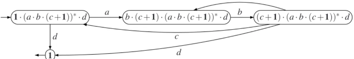
Example 3.8. Consider the automaton associated with the BPA∗_0,1(A_{)expression1·(a·b·(c+1))}∗_·d, (see Figure 2). It has a strongly connecting component with two exit states, both with one exit transition (d,1).

1·(a·b·(c+1))∗·d b·(c+1)·(a·b·(c+1))∗·d (c+1)·(a·b·(c+1))∗·d

1

a b

c

a

d

d

Figure 2: A non-trivial strongly connected component in BPA∗_0,1(A_{)with multiple exit transitions.}

Non-trivial strongly connected components in BPA∗_0,1(A_{) arise from executing the argument of a} Kleene star. An exit state of a strongly connected component in BPA∗_0,1(A_{)is then a state in which the} execution has the option to terminate. Due to the presence of0in BPA∗_0,1(A_{)this is, however, not the} only type of exit state in BPA∗_0,1(A_{)strongly connected components.}

Example 3.9. Consider the automaton associated with the BPA∗_0,1(A_)expression1·(a·((b·0) +1))∗· c (see Figure 3). The strongly connected component contains two exit states and two (distinct) exit transitions. One of these exit transitions leads to a deadlocked state.

1·(a·((b·0) +1))∗·c ((b·0) +1)·(a·((b·0) +1))∗·c

0·(a·((b·0) +1))∗·c

1

a

b

c a c

Figure 3: A strongly connected component with normed exit transitions.

The preceding example illustrates that the special property of strongly connected components in BPA∗_0,1(A_{)that we are after, should exclude from consideration any exit transition arising from an} oc-currence of0. This is achieved in the following definitions.

Definition 3.10. LetCbe a strongly connected component and lets∈C. An exit transition(a,s′)from

sisnormedifs′is normed. We denote byETn(s)the set of normed exit transitions froms. An exit states∈Cisaliveifs↓or there exists a normed exit transition froms.

Lemma 3.11. If p·q∗−→∗r, then either there exists p′ such that p−→∗p′andr=p′·q∗or there exist p′andq′such thatp−→∗_p′_{, p}′_↓,q−→∗_q′_{, andr=q}′_·q∗_.

Lemma 3.12. IfCis a basic strongly connected component, thenETn(p) =/0 for all p∈C.

Lemma 3.13. LetCbe a non-trivial strongly connected component in BPA∗_0,1(A_{), letp∈C, and letqbe} a BPA∗_0,1(A_{)process expression such thatC·qis a strongly connected component. Then p·qis an alive} exit state inC·qiffpis an alive exit state inCandqis normed.

Lemma 3.14. LetCbe a non-trivial strongly connected component in BPA∗_0,1(A_{), letp∈C, and letqbe} a normed BPA∗_0,1(A_{)process expression such thatC·qis a strongly connected component. Then}

ETn(p·q) =

ETn(p)·q∪ {(a,r)|r6∈C·q∧ris normed∧q−→a r} ifp↓; and

ETn(p)·q ifp6 ↓.

Proposition 3.15. LetCbe a non-trivial strongly connected component in BPA∗_0,1(A_{). Ifp1 and p2are} alive exit states inC, thenETn(p1) =ETn(p2).

Proof. Suppose thatp1and p2are alive exit states; we prove by induction on the structure of non-trivial

strongly connected components in BPA∗_0,1(A_{)as given by Proposition 3.6 thatETn(p1) =ETn(p2)and} p1↓iffp2↓.

IfCis basic, then by Lemma 3.12ETn(p1) =/0=ETn(p2), and, since p1and p2are alive exit states,

it also follows from this that bothp1↓and p2↓.

Suppose thatC=C′·q, withC′ a non-trivial strongly connected component, and let p′₁,p′₂∈C′ be such thatp1=p′₁·qand p2=p′₂·q. Since p1and p2are alive exit states, by Lemma 3.13 so arep′₁and

p′₂. Hence, by the induction hypothesis, ETn(p′1) =ETn(p′2)and p′1↓ iff p′2↓. From the latter it follows

that p1↓iffp2↓. We now apply Lemma 3.14: if, on the one hand, p1↓and p2↓, then

ETn(p1) =ETn(p′1)·q∪ {(a,r)|r6∈C∧ ∃r′.q

a

−→r−→∗r′↓}

=ETn(p′₂)·q∪ {(a,r)|r6∈C∧ ∃r′.q−→a r−→∗r′↓}=ETn(p2) ,

and if, on the other hand,p16 ↓and p26 ↓, thenETn(p1) =ETn(p′1)·q=ETn(p′2)·q=ETn(p2).

p0 p1

p2 p3

a

b

a

b

c c

Figure 4: A PA∗_0,1(A_{)-expressible automaton that is not expressible in BPA}∗ 0,1(A).

The PA∗_0,1(A_{)expression p0=1·(a·b)}∗_{kcgives rise to the automaton shown in Figure 4. It has} a strongly connected componentC={p0,p1}of which the alive exit states have different normed exit

transitions. Hence, by Proposition 3.15,p0is not BPA∗0,1(A)-expressible.

Theorem 3.16. BPA∗_0,1(A_{)is less expressive than PA}∗ 0,1(A).

4

Relative Expressiveness of

PA

(

A

₎

_and

_ACP

0,1

(

A

,

γ

)

The proof in [4] that PA∗_δ(A_{)is less expressive than ACP}∗₍A_,γ_{) uses the same expression as the one} showing that BPA∗_δ(A_{)is less expressive than PA}∗

δ(A), but it presupposes thatγ(c,d) =e. It is claimed

that the associated automaton fails the following general property of cycles in PA∗_δ(A_):

IfCis a cycle reachable from a PA∗₀(A_{)process term and there is a state inCwith a transition} to a terminating state, then all other states inChave only successors inC.

Example 4.1. Consider the PA∗_0,1(A_{)expression(a·(b+b·b))}∗_{·d, from which the cycle}

C={1·(a·(b+b·b))∗·d, (b+b·b)·(a·(b+b·b))∗·d}

is reachable. Clearly, the first expression inC can perform ad-transition to1. Then, according to the property above, every other expression only has transitions to expressions inC. However,

(b+b·b)·(a·(b+b·b))∗·d−→b b·(a·(b+b·b))∗·d6∈C .

If we replace, in the property above, the notion of cycle by the notion of strongly connected compo-nent, then the resulting property does hold for PA∗₀(A_{), but it still fails for PA}∗

0,1(A).

Example 4.2. Consider the PA∗_0,1(A_{) expression (a·b)}∗ _{kcit gives rise to the following non-trivial} strongly connected component: {1·(a·b)∗kc, b·(a·b)∗ kc}. The expression 1·(a·b)∗ kccan do a c-transition to1·(a·b)∗k1, for which the termination predicate holds, but at the same timeb·(a·b)∗kc has an exit transition(c,b·(a·b)∗k1).

In this section we shall establish that PA∗_0,1(A_{)is less expressive than ACP}∗

0,1(A,γ). To this end, we apply the same method as in Section 3. First, we syntactically characterise the non-trivial strongly con-nected components associated with PA∗_0,1(A_{)expressions. Then, we conclude that a weakened version} of the aforementioned property for strongly connected components holds in PA∗_0,1(A_{), and present an} ACP∗_0,1(A_,γ_{)expression that does not satisfy it.}

4.1 Strongly Connected Components inPA∗_0,1(A₎

To give a syntactic characterisation of the non-trivial strongly connected components in PA∗_0,1(A_{), we} reason again about the operational semantics. First, we extend the measure #( ) from Section 3 to PA∗_0,1(A_{)expressions.}

Definition 4.3. Letpbe a PA∗_0,1(A_{)expression; #(p)is defined with recursion on the structure of pby} the clauses (i)–(iv) in Definition 3.2 with the following clause added:

(v) #(pkq) =0.

With the extension, the non-increasing measure #( )still in most cases decreases over transitions.

Lemma 4.4. If pand p′are PA∗_0,1(A_{)expressions such that p−→}+_p′_{, then #(p)≥#(p}′_{). Moreover, if} #(p) =#(p′), then either p=p1·qand p′ =p′1·q, or p= p1k p2 and p′= p′1kp′2 for some process

expressions p1, p2, p′1,p′2, andq.

Lemma 4.5. Let p, q and r be PA∗_0,1(A_{) process expressions such that pkq−→}∗_{r. Then there exist} PA∗_0,1(A_{)process expressionsp}′ _andq′ _{such thatr=p}′_kq′_{, p−→}∗_p′_andq−→∗_q′_.

Let P and Q be sets of process expressions; by PkQ we denote the set of process expressions PkQ={pkq|p∈P∧q∈Q}. We also writePkqand pkQforPk {q}and{p} kQ, respectively.

The proof of the following lemma, characterising the syntactic form of non-trivial strongly connected components in PA∗_0,1(A_{), is a straightforward adaptation and extension of the proof of Lemma 3.4, using} Lemma 4.4 and Lemma 4.5 instead of Lemma 3.3.

The notion ofbasic strongly connected component in PA∗_0,1(A_{) is obtained from Definition 3.5 by} replacing BPA∗_0,1(A_{)by PA}∗

0,1(A)everywhere in the definition. In Proposition 3.6 we gave an inductive characterisation of non-trivial strongly connected components in BPA∗_0,1(A_{). There is a similar inductive} characterisation of non-trivial strongly connected components in PA∗_0,1(A_{), obtained by adding a case} for parallel composition.

Proposition 4.7. LetC be a non-trivial strongly connected component in PA∗_0,1(A_{). Then one of the} following holds:

(i) Cis a basic strongly connected component; or

(ii) there exist a non-trivial strongly connected componentC′ and a PA∗_0,1(A_{)expression qsuch that} C=C′·q; or

(iii) there exist strongly connected componentsC1andC2, at least one of them non-trivial, such that

C=C1kC2.

Note that, in the above proposition, one of the strongly connected componentsC1 andC2 may be

trivial in which case it consists of a single PA∗_0,1(A_)expression.

4.2 PA∗_0,1(A_)≺ACP∗

0,1(A,

γ

In Section 3 we deduced, from our syntactic characterisation of strongly connected components in BPA∗_0,1(A_{), the property that all alive exit states of a strongly connected component have the same sets} of normed exit transitions. This property may fail for strongly connected components in PA∗_0,1(A_{): the} automaton in Figure 4 is PA∗_0,1(A_{)-expressible, but the alive exit states p0 and p1 of the strongly} con-nected component {p0,p1} have different normed exit transitions. Note, however, that these normed

exit transitions both end up in another strongly connected component{p2,p3}. It turns out that we can

relax the requirement on normed exit transitions from strongly connected components in BPA∗_0,1(A_)to get a requirement that holds for strongly connected components in PA∗_0,1(A_{). The idea is to identify exit} transitions if they have the same action and end up in the same strongly connected component.

Definition 4.8. LetT_{= (S,→,↓)be an}A_{-labelled transition system space. We define a binary relation} ∼onA_{×Sby(a,s)∼(a}′_,s′_)iffa=a′_andsands′_{are in the same strongly connected component in}T_.

Since the relation of being in the same strongly connected component is an equivalence on states in a transition system space, it is clear that∼is an equivalence relation on exit transitions. The following lemma will give some further properties of the relation∼associated with PA∗_0,1(A_).

Lemma 4.9. Let pand qbe PA∗_0,1(A_{) expressions, and letaand b be actions. If(a},p)∼(b,q), then (a,p·r)∼(b,q·r),(a,pkr)∼(b,qkr), and(a,rkp)∼(b,rkq).

To formulate a straightforward corollary of this lemma we use the following notation: ifEis a set of exit transitionsEand pis a PA∗_0,1(A_{)expression, thenE·p,Ekpand pkEare defined by}

Ekp={(a,qkp)|(a,q)∈E} , and pkE={(a,pkq)|(a,q)∈E} .

We are now in a position to establish a property of strongly connected components in PA∗_0,1(A₎ that will allow us to prove that PA∗_0,1(A_{) is less expressive than ACP}∗

Lemma 4.10. LetC1 and C2 be sets of PA∗0,1(A) expressions. ThenC1kC2 is a strongly connected

component iff bothC1andC2are strongly connected components. Moreover,C1kC2is non-trivial iff at

least one ofC1andC2is non-trivial.

Lemma 4.11. LetC1andC2be a strongly connected components in PA∗0,1(A), both with alive exit states. ThenC1kC2is a strongly connected component with alive exit states too, and, for allp∈C1andq∈C2,

ETn(pkq) = (ETn(p)kq)∪(pkETn(q)).

To formulate the special property of strongly connected components in PA∗_0,1(A_{)that will allow us} to prove that some ACP∗_0,1(A_,γ_{)expressions do not have a counterpart in PA}∗

0,1(A), we need the notion of maximal alive exit state.

Definition 4.12. LetT_{= (S,→,↓)be an}A_{-labelled transition system space, let∼ ⊆}A_{×Sbe the} equiv-alence relation associated withT_{according to Definition 4.8, letCbe a strongly connected component} inT_{, and lets∈Cbe an alive exit state. We say thatsismaximal(modulo∼) if for all alive exit states} s′∈Cand for alle′∈ETn(s′)there exists an exit transitione∈ETn(s)such thate∼e′.

The following proposition establishes the property with which we shall prove that PA∗_0,1(A_{)is less} expressive than ACP∗_0,1(A,γ).

Proposition 4.13. IfCis a strongly connected component in PA∗_0,1(A_{)andChas an alive exit state, then} Chas a maximal alive exit state.

p0 p1

p4

p2 p3

p5

a

b

a

b d

d

c c

c e

Figure 5: An ACP∗_0,1(A_,γ_{)-expressible automaton that is not expressible in PA}∗ 0,1(A).

Supposeγ(b,c) =e; then the ACP∗_0,1(A,γ)expression p0=1·(a·b)∗·dkcgives rise to the

automa-ton shown in Figure 5. It has a strongly connected componentC={p0,p1}, and none of its alive exit

states is maximal. Hence, by Proposition 4.13,p0is not PA∗0,1(A)-expressible.

Theorem 4.14. PA∗_0,1(A_{)is less expressive than}S

γACP∗0,1(A,γ).

5

Every Finite Automaton is

ACP

(

A

_,

γ

₎

_-expressible

Milner observed in [10] that there exist finite automata that are not bisimilar to the finite automaton associated with a BPA∗_0,1(A_{)expression. Our proof of Theorem 3.16 has Milner’s observation as an} im-mediate consequence: the finite automaton associated with the PA∗_0,1(A_{)expression used in the proof is} not BPA∗_0,1(A_{)-expressible. Similarly, by Theorem 4.14, there are finite automata that are not expressible} in PA∗_0,1(A_).

state,” has control. Ana-transition from that current state to a next state corresponds with a communica-tion between two components. We make essential use of ACP∗_0,1(A_,γ_{)’s facility to let the actionabe the} result of communication.

Example 5.1. Consider the finite automaton in Figure 6.

s0 s1

s2 s3

a1

a0

a1

a2

a0

a1

a2

a0

a1

Figure 6: A finite automaton.

We associate with every statesian ACP∗0,1(A,γ)expression pias follows:

p0=

enter0·(leave0,1+leave1,1)

∗ _{, p}

2=

enter2·(leave0,0+leave1,3+1)

∗ _,

p1=

enter1·a1∗·(leave2,2)

∗ _{, p}

3=

enter3·0

∗ _.

Everypihas anenteritransition to gain control, and by executing aleavek,jit may then release control to pjwith actionakas effect. We define the communication function so that anenteriaction communicates with aleavek,i action, resulting in the actionak. Loops in the automaton (such as the loop on state s1)

require special treatment as they should not release control.

Let p′₀ be the result of executing theenter0-transition from p0. We define the ACP∗0,1(A,γ) expres-sion that simulates the finite automaton in Figure 6 as the parallel composition of p′₀, p1, p2 and p3,

encapsulating the control actionsenteriandleavek,i, i.e., as

∂{enteri,leavek,i|0≤i≤3,0≤k≤2}(p

′

0kp1kp2kp3) .

We now present the technique illustrated in the preceding example in full generality. Let F₌ (S,→,s0,↓) be a finite automaton, let S={s0, . . . ,sn}, and let A={a1, . . . ,am} be the set of actions

occurring on transitions inF_{. We shall associate with}F_{an ACP}∗

0,1(A,γ) expression pF that has

pre-cisely one parallel componentpifor every statesiinS. To allow a parallel component to gain and release control, we use a collection ofcontrol actions C, assumed to be disjoint fromA, and defined as

C={enteri|1≤i≤n} ∪ {leavek,i|1≤i≤n,1≤k≤m} .

Gaining and releasing control is modelled by the communication functionγsatisfying:

γ(enteri,leavek,j) =

ak ifi= j; and

undefined otherwise.

For the specification of the ACP∗_0,1(A_,γ_{)expressions piwe need one more definition: for 1≤i,j≤nwe} denote byKi,jthe set of indices of actions occurring as the label on a transition fromsi tosj, i.e.,

Ki,j={k|si−−→ak sj} .

Now we can specify the ACP∗_0,1(A_,γ_{)expressions pi (1≤i≤n) by}

pi=1·

enteri·(

∑

ak)∗·(

∑

1≤j≤n j6=i

∑

k∈Ki,j

leavek,i(+1)si↓)

By(+1)_s

i↓ we mean that the summand+1is optional; it is only included ifsi↓. The empty summation

denotes0. (We let pi start with1to get that the finite automaton associated withpF is isomorphic and

not just bisimilar withF_.)

Note that, in ACP∗_0,1(A,γ), everypihas a unique outgoing transition; specifically pi−−−−→enteri p′i, where p′_idenotes:

p′_i= (1·(

∑

ak)∗·(

∑

0≤j≤n j6=i

∑

k∈Ki,j

leavek,i(+1)_si↓))·pi.

We now define pF=∂C(p′0kp1k · · · kpn). Clearly, the construction of pF works for every finite

automatonF_{. The bijection defined bysi7→}∂_{C(p0k · · · kpi−1kp}′

ik pi+1k · · · kpn)is an isomorphism fromF_{to the automaton associated with pF by the operational semantics. We shall refer to pF as the} ACP∗_0,1(A_,γ_{)expression associated with}F_.

Theorem 5.2. LetF_{be a finite automaton, and let pF be its associated ACP}∗

0,1(A,γ)expression. The automaton associated withpFby the operational rules for ACP∗_0,1(A,γ)is isomorphic toF.

Corollary 5.3. For every finite automatonF_{there exists an instance of ACP}∗

0,1(A,γ)with a suitable finite set of actionsA_{and a handshaking communication function} γ _{such that}F _{is ACP}∗

0,1(A,γ)-expressible up to isomorphism.

6

Conclusion

In this paper we have investigated the effect on the expressiveness of regular expressions modulo bisim-ilarity if different forms of parallel composition are added. We have established an expressiveness hi-erarchy that can be briefly summarised as: BPA∗_0,1(A_)≺PA∗

0,1(A)≺

S

γACP∗0,1(A,γ). Furthermore, while not every finite automaton can be expressed modulo bisimilarity with a regular expression, it suffices to add a form of ACP(A_,γ_{)-style parallel composition, with handshaking communication and} encapsulation, to get a language that is sufficiently expressive to express all finite automata modulo bisimilarity. This result should be contrasted with the well-known result from automata theory that every non-deterministic finite automaton can be expressed with a regular expression modulo language equiva-lence.

As an important tool in our proof, we have characterised the strongly connected components in BPA∗_0,1(A_{) and PA}∗

0,1(A). An interesting open question is whether the two given characterisations are complete, in the sense that a finite automaton is expressible in BPA∗_0,1(A_{)or PA}∗

0,1(A)iff all its strongly connected components satisfy our characterisation. If so, then our characterisation would constitute a useful complement to the characterisation of [1] and perhaps lead to a more efficient algorithm for deciding whether a non-deterministic automaton is expressible.

In [4] it is proved that every finite transition system without intermediate termination can be denoted in ACP∗_0,τ(A_,γ_{) up tobranching bisimilarity [7], and that ACP}∗

0(A,γ) modulo (strong) bisimilarity is strictly less expressive than ACP∗_0,τ(A_,γ_{). In contrast, we have established that every finite automaton} (i.e., every finite transition system not excluding intermediate termination) is denoted by an ACP∗_0,1(A,γ)

expression. It follows that ACP∗_0,1(A_,γ_{)and ACP}∗

0,1,τ(A,γ)are equally expressive.

An interesting question that remains is whether it is possible to omit constructions from ACP∗_0,1(A_,γ₎ without losing expressiveness. We conjecture that∂H( )cannot be omitted without losing expressive-ness: encapsulatingcin the ACP∗_0,1(A_,γ_{)expression1·(a·b)}∗_{·bkc, which is used in Section 4 to show} that PA∗_0,1(A_{) is less expressive than ACP}∗

Acknowledgement We thank Leonardo Vito and the other participants of the Formal Methods seminar of 2007 for their contributions in an early stage of the research for this paper.

References

[1] J. C. M. Baeten, F. Corradini & C. A. Grabmayer (2007):A Characterization of Regular Expressions under Bisimulation.Journal of the ACM54(2).

[2] J. C. M. Baeten & R. J. van Glabbeek (1987):Merge and Termination in Process Algebra. In: Kesav V. Nori, editor:FSTTCS,Lecture Notes in Computer Science287, Springer, pp. 153–172.

[3] J. A. Bergstra, I. Bethke & A. Ponse (1994): Process Algebra with Iteration and Nesting. The Computer Journal37(4), pp. 243–258.

[4] J. A. Bergstra, W. Fokkink & A. Ponse (2001):Process Algebra with Recursive Operations. In: J. A. Bergstra, A. J. Ponse & S. A. Smolka, editors:Handbook of Process Algebra, Elsevier, pp. 333–389.

[5] J. A. Bergstra & J. W. Klop (1984): Process algebra for synchronous communication. Information and Control1/3(60), pp. 109–137.

[6] T. H. Cormen, C. E. Leiserson, R. L. Rivest & C. Stein (2001):Introduction to Algorithms. MIT Press, 2nd edition.

[7] R. J. van Glabbeek & W. P. Weijland (1996): Branching Time and Abstraction in Bisimulation Semantics. Journal of the ACM43(3), pp. 555–600.

[8] J .E. Hopcroft, R. Motwani & J. D. Ullman (2006):Introduction to Automata Theory, Languages, and Com-putation. Pearson.

[9] C. J. P. Koymans & J. L. M. Vrancken (1985):Extending process algebra with the empty processε. Logic Group Preprint Series 1, State University of Utrecht.

[10] R. Milner (1984): A Complete Inference System for a Class of Regular Behaviours. Journal of Comput. System Sci.28(3), pp. 439–466.

[11] R. Milner (1989):Communication and Concurrency. Prentice-Hall International, Englewood Cliffs. [12] D. Park (1981):Concurrency and automata on infinite sequences. In: P. Deussen, editor:Proc. of the 5th GI

Conference, LNCS 104, Springer-Verlag, Karlsruhe, Germany, pp. 167–183.

[13] G. D. Plotkin (2004):A structural approach to operational semantics. J. Log. Algebr. Program.60-61, pp. 17–139.