An accuracy assessment of the CALIOP/CALIPSO version 2 aerosol extinction product based on a detailed multi-sensor, multi-platform case study

(1)

ACPD

10, 27967–28015, 2010

CALIOP version 2 aerosol extinction

product

M. Kacenelenbogen et al.

Title Page

Abstract Introduction

Conclusions References

Tables Figures

◭ ◮

Back Close

Full Screen / Esc

Printer-friendly Version

Interactive Discussion

Discussion

P

a

per

|

Dis

cussion

P

a

per

|

Discussion

P

a

per

|

Discussio

n

P

a

per

|

Atmos. Chem. Phys. Discuss., 10, 27967–28015, 2010 www.atmos-chem-phys-discuss.net/10/27967/2010/ doi:10.5194/acpd-10-27967-2010

Atmospheric Chemistry and Physics Discussions

This discussion paper is/has been under review for the journal Atmospheric Chemistry and Physics (ACP). Please refer to the corresponding final paper in ACP if available.

An accuracy assessment of the

CALIOP/CALIPSO version 2 aerosol

extinction product based on a detailed

multi-sensor, multi-platform case study

M. Kacenelenbogen1, M. A. Vaughan2, J. Redemann3, R. M. Hoff4, R. R. Rogers2, R. A. Ferrare2, P. B. Russell5, C. A. Hostetler2, J. W. Hair2, and B. N. Holben6

1

ORAU/ NASA Ames Research Center, Moffett Field, CA, USA

2

NASA Langley Research Center, Hampton, VA, USA

3

Bay Area Environmental Research Institute, Sonoma, CA, USA

4

Joint Center for Earth Systems Technology (JCET)/Goddard Earth Science and Technology Center (GEST), University of Baltimore County, MA, USA

5

NASA Ames Research Center, Moffett Field, CA, USA

6

NASA Goddard Space Flight Center, Greenbelt, MA, USA

(2)

ACPD

10, 27967–28015, 2010

product

Title Page

Tables Figures

◭ ◮

Back Close

Full Screen / Esc

Discussion

P

a

per

|

Dis

cussion

P

a

per

|

Discussion

P

a

per

|

Discussio

n

P

a

per

|

Abstract

The Cloud Aerosol LIdar with Orthogonal Polarization (CALIOP), on board the CALIPSO platform, has measured profiles of total attenuated backscatter coefficient (level 1 products) since June 2006. CALIOP’s level 2 products, such as the aerosol backscatter and extinction coe_fficient profiles, are retrieved using a complex succes-5

sion of automated algorithms. The goal of this study is to help identify potential short-comings in the CALIOP version 2 level 2 aerosol extinction product and to illustrate some of the motivation for the changes that will be introduced in the next version of CALIOP data (version 3, currently being processed). As a first step, we compared CALIOP version 2-derived AOD with the collocated MODerate Imaging Spectrora-10

diometer (MODIS) AOD retrievals over the Continental United States. The best sta-tistical agreement between those two quantities was found over the Eastern part of the United States with, nonetheless, a weak correlation (R∼0.4) and an apparent CALIOP

version 2 underestimation (by∼66 %) of MODIS AOD. To help quantify the potential

factors contributing to the uncertainty of the CALIOP aerosol extinction retrieval, we 15

then focused on a one-day, multi-instrument, multiplatform comparison study during the CALIPSO and Twilight Zone (CATZ) validation campaign on August 04, 2007. This case study illustrates the following potential reasons for a bias in the CALIOP AOD: (i) CALIOP’s low signal-to-noise ratio (SNR) leading to the misclassification and/or lack of aerosol layer identification, especially close to the Earth’s surface; (ii) the cloud contam-20

(3)

ACPD

10, 27967–28015, 2010

product

Title Page

Tables Figures

◭ ◮

Back Close

Full Screen / Esc

Discussion

P

a

per

|

Dis

cussion

P

a

per

|

Discussion

P

a

per

|

Discussio

n

P

a

per

|

1 Introduction

The Cloud Aerosol LIdar with Orthogonal Polarization (CALIOP), on board the CALIPSO platform (flying as part of the A-Train satellite constellation since April 2006), is a three-channel elastic backscatter lidar optimized for aerosol and cloud profiling. CALIOP measures high-resolution (1/3 km in the horizontal and 30 m in the vertical in 5

low and middle troposphere) profiles of the attenuated backscatter by aerosols and clouds at visible (532 nm) and near-infrared (1064 nm) wavelengths along with polar-ized backscatter in the visible channel (Winker et al., 2009). These data are distributed as part of the level 1 CALIOP products. The level 2 CALIOP products are derived from the level 1 measurements using a complex and intricate succession of algorithms that 10

are described in detail in a special issue of the Journal of Atmospheric and Oceanic Technology (e.g., Winker et al., 2009). The level 2 retrieval scheme is composed of a feature detection scheme, a module that classifies features according to layer type (e.g., cloud vs. aerosol) and sub-type, and, finally, an extinction retrieval algorithm that estimates the aerosol backscatter, the extinction coefficient profile and total column 15

aerosol optical depth (AOD) for an assumed extinction-to-backscatter ratio (also called S_a) for each detected aerosol layer.

For a select list of observables, CALIOP attenuated backscatter, aerosol backscatter and extinction coefficient profiles have been shown to yield reasonable agreement with ground-based (Kim et al., 2008; Mamouri et al., 2009; Mona et al., 2009; Pappalardo 20

et al., 2010) and airborne lidar measurements (McGill et al., 2007; Omar et al., 2009; Rogers et al., 2010). For example, Pappalardo et al. (2010) have observed a mean percentage di_fference of less than 20% between level 1 CALIOP and ground-based EARLINET (European Aerosol Research Lidar Network) lidar measurements of attenu-ated backscatter profiles since June 2006 over Europe, showing an absence of evident 25

(4)

ACPD

10, 27967–28015, 2010

product

Title Page

Tables Figures

◭ ◮

Back Close

Full Screen / Esc

Discussion

P

a

per

|

Dis

cussion

P

a

per

|

Discussion

P

a

per

|

Discussio

n

P

a

per

|

Resolution Lidar (HSRL) (Hair et al., 2008) acquired since June 2006. Results show HSRL and CALIOP (version 2) 532 nm total attenuated backscatter agree within 1.1%

±23% for daytime lighting conditions in the free troposphere. Kim et al. (2008) showed that CALIOP, when compared to a ground-based lidar in Korea, has detected cloud and aerosol top/base layers and retrieved the aerosol extinction profiles correctly within re-5

spectively 0.10 km and 30% in cloud-free nighttime and semi-transparent cirrus cloud conditions. According to Omar et al. (2009), CALIOP (Version 2) generally overesti-mates the HSRL extinction measurements for several case studies, with an average extinction bias of 0.003 km−1 (∼24%) during the CALIPSO and Twilight Zone (CATZ) validation campaign and 0.015 km−1 (∼59%) during the Gulf of Mexico Atmospheric

10

Composition and Climate Study (GoMACCS).

Nonetheless, there are significant uncertainties associated with the version 2 CALIOP aerosol extinction and backscatter retrievals, and these are not well-quantified in any ancillary quality assurance information included in the level 2 data files. These uncertainties are introduced by several di_fferent factors that are often related to each 15

other (Winker et al., 2009; Yu et al., 2010). First of all, the CALIOP layer detection scheme will most likely fail to detect layers with aerosol backscatter coe_fficients falling below a sensitivity threshold of 2∼4×10−4km−1sr−1 in the troposphere (Winker et

al., 2009). Consequently, if we assume a lidar extinction-to-backscatter ratio (S_a) of 50 sr, the minimum detectable extinction coe_fficient is in the neighborhood of 0.01 to 20

0.02 km−1 _{(corresponding to a lowest detectable AOD of 0.02–0.04 in a homogenous} 2 km planetary boundary layer). A second significant source of error is the lack of pho-tons returned from underneath highly attenuating layers, such as dense aerosol and cloud layers. This may result in the erroneous or total lack of aerosol identification in the lower part of a given profile. In such situations, the CALIOP detection algorithm can 25

(5)

ACPD

10, 27967–28015, 2010

product

Title Page

Tables Figures

◭ ◮

Back Close

Full Screen / Esc

Discussion

P

a

per

|

Dis

cussion

P

a

per

|

Discussion

P

a

per

|

Discussio

n

P

a

per

|

errors can also occur in the aerosol subtyping algorithm (Omar et al., 2009), leading to an incorrect assumption about the appropriate extinction-to-backscatter ratio. The CALIOP AOD fractional error is similar to the S_afractional error for small AOD values (Winker et al., 2009). On the other hand, as the AOD increases, the AOD fractional error will quickly become much higher than the S_afractional error. For example, a frac-5

tional error of 30% for S_a would result in an AOD fractional error of∼50% for an AOD of 0.5 and nearly 100% for an AOD of 1.

Despite these uncertainties, there have been a number of publications using CALIOP version 2 level 2 data in a qualitative or even quantitative manner. Focusing on arti-cles published in 2010, some authors recognize the largely unvalidated nature of level 10

2 version 2 data. Among those, there have been attempts to produce more accurate CALIOP data by applying further cloud-screening (Sekiyama et al., 2010) or even an intensive data screening scheme (Yu et al., 2010). Some mention the uncertainties associated with the level 2 version 2 data but apply no specific filtering (e.g., Peyridieu et al., 2010; Jones et al., 2009). We note that many articles in 2010 (and probably a 15

few more in the previous years) omit discussions on the accuracy of level 2 version 2 CALIOP data. This is, for example, the case for Gonzi et al. (2010), who qualitatively compared biomass burning injection height estimates from the GEOS-Chem model to unfiltered CALIOP vertical feature mask data. This latter product is also used to suggest the presence of an extended aerosol layer over central India that could be 20

associated with agriculture crop residue burning activities (Sharma et al., 2010), and to help determine the altitude of smoke plumes over the US during Summer 2006 (McMillan et al., 2010). Finally, Kuhlmann et al. (2010) make more intensive use of the unfiltered level 2 CALIOP aerosol layer product to draw conclusions regarding the par-ticle type and general aerosol vertical distribution during the Asian summer Monsoon. 25

(6)

ACPD

10, 27967–28015, 2010

product

Title Page

Tables Figures

◭ ◮

Back Close

Full Screen / Esc

Discussion

P

a

per

|

Dis

cussion

P

a

per

|

Discussion

P

a

per

|

Discussio

n

P

a

per

|

In this study we attempt to assess the consistency between the CALIOP AOD re-trievals and comparative aerosol observations from multiple sources and platforms (in-cluding ground-based, airborne and satellite instruments). As a first step, we compare MODIS (MODerate Imaging Spectroradiometer, collection 5) and CALIOP total column AOD over the United States for a period of four months during the summer of 2007 5

in an attempt to assess the general consistency between the two satellite instruments. Let us point out that Levy et al. (2010) demonstrate the global validation of total MODIS AOD over dark-land targets with more than 66% of MODIS AOD matching those of the AErosol RObotic NETwork (AERONET, Level 2 measurements at over 300 sites) within the expected uncertainty defined by∆AOD=±0.05±0.15 AOD. We find a general

un-10

derestimate of the MODIS-derived AOD by CALIOP and discuss possible explanations for the observed discrepancies in Sect. 3. In Sect. 4, we then focus on a one-day, multi-sensor case study that yielded AOD differences similar to the mean differences found in our broader MODIS-CALIOP comparison. This case study was part of the nine ground-based CATZ field campaigns (each campaign occurring on separate days 15

between 26 June and 29 August 2007) in Virginia and Maryland, when four AERONET sites were deployed and the NASA Langley Research Center airborne HSRL was flown along the daytime CALIOP track, with coincident space-borne observations available from MODIS and POLDER (Polarization and Directionality of Earth’s Reflectances). The detailed suborbital observations, and in particular, the comparison of coincident 20

CALIOP and HSRL profiles, are used to explore the following potential reasons for the overall bias between the MODIS AOD and the CALIOP version 2 AOD product: (i) CALIOP’s low Signal to Noise Ratio (SNR) which can lead to the misclassification and/ or lack of aerosol layer identification, especially close to the Earth’s surface; (ii) the cloud contamination of CALIOP aerosol backscatter and extinction profiles; (iii) a po-25

tentially erroneous S_a assumption in CALIOP’s extinction retrieval and (iv) calibration errors in the CALIOP daytime attenuated backscatter coe_fficient profiles.

(7)

ACPD

10, 27967–28015, 2010

product

Title Page

Tables Figures

◭ ◮

Back Close

Full Screen / Esc

Discussion

P

a

per

|

Dis

cussion

P

a

per

|

Discussion

P

a

per

|

Discussio

n

P

a

per

|

are being introduced in the next version of CALIOP data (Version 3, released in May 2010). Based on the multi-instrument, multi-platform comparison study, we seek to quantify the major factors contributing to the uncertainty of the CALIOP aerosol extinc-tion retrieval. We submit that the identificaextinc-tion and discussion of retrieval uncertainties provided here will help understand and interpret the results obtained in previous studies 5

like the ones cited above.

2 Instruments

2.1 Aeronet

The AErosol RObotic NETwork (AERONET) (Holben et al., 1998) is composed of auto-matic sun-sky scanning spectral radiometers. The AOD and ˚Angstr ¨om exponent (called 10

˚

A, expresses the wavelength dependence,λ, of the AOD and is defined as the slope of the first order linear regression of log(AOD) versus log(λ)) are determined by direct sun measurements. The aerosol size distribution and optical parameters (such as the single scattering albedo, volume concentration, refractive index, etc.) are derived from the angular distribution of sky radiances measured in the almucantar according to the 15

algorithm developed by Dubovik and King (2000a). In this study, we use version 2-level 1.5 AERONET data (Smirnov et al., 2002). During the CATZ field experiment, the AERONET sunphotometer observations were sampled more frequently than in the case of the standard automatic mode measurement protocol (Holben et al., 1998), preventing the data from being labeled level 2. However, the correct calibration of the 20

sunphotometers during the experiment results in the same estimated total uncertainty in the direct AOD measurements as for the level 2 data: ∼0.010–0.021 (Eck et al.,

1999). In the case of AOD values above 0.2 at 440 nm, Dubovik et al. (2000b) reports accuracies of 0.03 for the single scattering albedo, 0.02–0.04 for the real part of the refractive index, 30% (50%) of the imaginary part of the refractive index in case of 25

(8)

ACPD

10, 27967–28015, 2010

product

Title Page

Tables Figures

◭ ◮

Back Close

Full Screen / Esc

Discussion

P

a

per

|

Dis

cussion

P

a

per

|

Discussion

P

a

per

|

Discussio

n

P

a

per

|

radius between 0.1 and 7 µm (lower than 0.1 µm or above 7 µm). In the case of lower AOD values (AOD(440)≤0.2), the accuracy levels drop down to 0.05–0.07 for SSA,

80%–100% for the imaginary part of the refractive index, and 0.05 for the real part of the refractive index.

2.2 CALIOP 5

CALIOP on the CALIPSO platform employs a linearly polarized laser that transmits pulses at 532 nm and 1064 nm. The two 532 nm receiver channels separately measure the components of the 532 nm backscatter signal polarized parallel and perpendicular to the outgoing beam. The measured CALIOP attenuated backscatter coe_fficient at wavelengthλand range z,β_λ′(z), can be written as:

10

β′

λ(z)=(βa,λ(z)+βm,λ(z))T

2

λ(z) (1)

whereβa,λ andβm,λ are, respectively, the aerosol and molecular retrieved backscatter

coefficient profile, andT_λ2=T_a,λ2 T_m,λ2 T_O2

3,λis the atmospheric two-way transmittance (i.e.,

signal attenuation) due to aerosols, molecular scattering, and absorbing gases such as ozone.

15

The aerosol transmittance between the lidar calibration region and range z, T_a,λ(z), can be expressed as follows:

T_a,λ2 (z)=exp 

−2

z

Z

z0

α_a,λ(z)d z 

=exp(−2τ_a,λ) (2)

wherez₀is the height of the calibration region,αa,λis the aerosol extinction coefficient

andτ_a,λ, the aerosol optical depth. 20

We will be concentrating mostly on the CALIOP-measured total attenuated backscat-ter coe_fficients, β

′

(9)

ACPD

10, 27967–28015, 2010

product

Title Page

Tables Figures

◭ ◮

Back Close

Full Screen / Esc

Discussion

P

a

per

|

Dis

cussion

P

a

per

|

Discussion

P

a

per

|

Discussio

n

P

a

per

|

the retrieved aerosol extinction coefficient profiles,αa,532(z) along the CALIOP ground track.

The extinction coefficient profiles are retrieved using a globally automated feature recognition algorithm that assumes a range-invariant extinction-to-backscatter ratio, also referred to as lidar ratio (S_a,₅₃₂₌αa,532(z)/βa,532(z)) for each layer detected. The 5

CALIOP value of S_a₅₃₂ used for any layer depends on the geographical location, the integrated attenuated backscatter color ratio, the layer-integrated volume depolariza-tion ratio, and a general Look Up Table (LUT) (Liu et al., 2009; Omar et al., 2009). The prelaunch goal of the CALIPSO mission was to retrieve aerosol extinction coeffi -cients accurate to within±40% (Winker et al., 2003). We have attributed names to all

10

the CALIOP parameters used in this study. They are listed in Table 1 along with the standard variables, original file name, level, and spatial resolution due to averaging.

CALIOP’s version 2 data products do not provide uncertainty estimates for retrieved optical parameters such as AOD and extinction coe_fficients. The uncertainties at-tributed to the CALIOP aerosol optical depths can be obtained by applying an error 15

estimator algorithm to the quantities reported in the aerosol layer products, taking into account the relative error on the lidar ratio, the calibration coe_fficient and the SNR for each detected aerosol layer. The error on the SNR may be slightly more complex to estimate as it depends on the backscatter intensity, the lighting conditions (i.e., day vs. night), and the amount of horizontal averaging applied to the initial attenuated 20

backscatter profiles.

2.3 HSRL

Retrieval of aerosol extinction profiles using the standard elastic backscatter lidar technique requires either a measurement of AOD to constrain the extinction retrieval (Young, 1995; McGill et al., 2003) or an assumption on the aerosol extinction-to-25

(10)

ACPD

10, 27967–28015, 2010

product

Title Page

Tables Figures

◭ ◮

Back Close

Full Screen / Esc

Discussion

P

a

per

|

Dis

cussion

P

a

per

|

Discussion

P

a

per

|

Discussio

n

P

a

per

|

type (Hair et al., 2008). The HSRL technique is typically employed for the 532 nm wavelength utilizing the iodine vapor filter technique (Hair et al., 2001, 2008; Piironen et al., 1994). The received 532 nm backscatter return is split between three optical channels: (1) one measuring the backscatter (predominantly aerosol) polarized or-thogonally to the transmitted polarization, (2) one measuring 10% of the molecular and 5

aerosol backscatter polarized parallel to the transmitted polarization, and (3) one pass-ing through an iodine vapor cell which absorbs the central portion of the backscatter spectrum, including all of the Mie backscatter, and transmits only the Doppler/pressure-broadened molecular backscatter. This third channel, (the “molecular channel”) is used to retrieve the extinction profile and all three channels are used to retrieve profiles of 10

aerosol backscatter and extinction coe_fficients and aerosol depolarization ratios. Hair et al. (2008) described the potential errors introduced in any of these quantities and found the 532 nm extinction systematic errors to be less than 0.01 km−1 for typical aerosol loading. Table 2 describes the HSRL analyzed data products used in this study. We use an HSRL subset file with a∼4/3 km horizontal and 30 m vertical

resolu-15

tion. The∼4/3 km horizontal resolution of the HSRL aerosol backscatter (e.g. extinction

and lidar ratio) coe_fficient profiles is obtained by computing 10 (e.g. 60) second running averages of the raw data (initially sampled at 2 Hz), then decimating the results by a factor of 20.

2.4 POLDER and MODIS 20

POLDER-3 (POLarization and Directionality of Earth’s Reflectances, 3rd version of the instrument, on board the PARASOL platform) and MODIS (on board the Earth Observ-ing System (EOS) AQUA satellite) are both passive radiometers, with both platforms being simultaneously part of the A-Train during five years (December 2004–2009), in-cluding our study period of Summer 2007. POLDER’s strength is the measurement 25

(11)

ACPD

10, 27967–28015, 2010

product

Title Page

Tables Figures

◭ ◮

Back Close

Full Screen / Esc

Discussion

P

a

per

|

Dis

cussion

P

a

per

|

Discussion

P

a

per

|

Discussio

n

P

a

per

|

the 865 nm channel. MODIS AOD is retrieved over oceans in 7 different spectral bands (6₊ extrapolated) from the visible to the near infrared and over land in 3 bands (2₊1 interpolated). POLDER’s spatial resolution is 5×6.5 km (500×500 m for MODIS) and its wide field of view induces a 1600 km swath (2330 km for MODIS) that allows a nearly global daily coverage. To increase the signal to noise ratio, the standard retrieval al-5

gorithm is applied to 3×3 POLDER pixels (20×20 for MODIS), leading to a resolution in the aerosol AOD of 15×19.5 km (10×10 km for MODIS). The AOD retrieval from

the POLDER polarized measurements is described by Deuz ´e et al. (2001) and the MODIS AOD retrieval algorithm over land is described in Kaufmann and Tanr ´e (1998). The polarization by aerosols mainly comes from small spherical particles in the accu-10

mulation mode (Vermeulen et al., 2000), indicating that POLDER-derived AOD is well suited for remote sensing of fine mode particles. Validation studies suggest that the expected uncertainty on the MODIS AOD over dark land surfaces could be represented by_∆AOD₌±0.05±0.15 AOD (Levy et al., 2010).

3 Evaluation of Version 2 CALIOP extinction retrieval: summer 2007 15

In this study, for convenience, all satellite data are remapped on the 12×12 km

Com-munity Multiscale Air Quality (CMAQ) model grid (US EPA, 1999). Each MODIS 10×10 km cell center has been attributed to the closest CMAQ cell center. In the case of CALIOP, the product to be remapped is the standard level 2 extinction coefficient, αa,532@40 km (see Table 1). CALIOP provides one constant extinction vertical profile 20

between start-location l_start and end-location l_end, with a horizontal distance of 40 km between l_start and l_end. In addition, eachα_a,₅₃₂@40 km profile is separated from adja-cent profiles by a distance of 1/3 km along the CALIOP track. A 12×12 km CMAQ cell

can then contain, at the most, two di_fferent parts of α_a,₅₃₂@40 km profiles. When the CMAQ cell contains only one α_a,₅₃₂@40 km profile, this profile is simply attributed to 25

(12)

ACPD

10, 27967–28015, 2010

product

Title Page

Tables Figures

◭ ◮

Back Close

Full Screen / Esc

Discussion

P

a

per

|

Dis

cussion

P

a

per

|

Discussion

P

a

per

|

Discussio

n

P

a

per

|

αa,532@40 km profiles weighted by the number of correspondingβ

′

532@1/3 km profiles contained in the cell. The CALIOP AOD data value for each cell is then obtained by integrating its correspondingαa,532@40 km profile on the vertical.

We start this study by comparing MODIS and CALIOP AOD values over the con-tinental United States from June to September 2007. Multiple constraints have been 5

applied to the data sets for this study. First of all, we have kept only positive MODIS AOD and CALIOP αa,532@40 km values. Secondly, for rigorous cloud-clearing and the elimination of outliers, the CALIOP β_a,₅₃₂@40 km data are required to be be-low 0.011 sr−1km−1 (a value typically found for a polluted continental or biomass burning type of aerosol with an extinction-to-backscatter lidar ratio of 70 sr and an 10

α_a,₅₃₂@40 km value of 0.8 km−1, corresponding to a visibility of >∼5 km). Finally,

CALIOP AOD values are computed only when aerosol is detected in 20 or more vertical bins within a 40- km averaged profile. According to Table 1, the vertical resolution of the CALIOPα_a,₅₃₂@40 km product is 120 m (below 8 km). Hence, the 20-bin requirement on the vertical translates into a minimum layer thickness of 2.4 km, assuming these 15

points are consecutive within a profile.

Figure 1 shows the MODIS-CALIOP AOD comparison over the entire United States (on the left) and over the Eastern part of the US (on the right, longitude above−100◦).

Each data set has been arranged in twenty di_fferent MODIS and CALIOP AOD bins. Figure 1 shows the corresponding data count for each bin center. The red lines on 20

Fig. 1a and b show the first principal component regression (Kendall, 1957) that fits a line by minimizing MODIS and CALIOP AOD residuals simultaneously while giving both data sets equal weight.

According to Fig. 1, the statistical agreement between MODIS and CALIOP AOD is slightly better over the Eastern part of the United States (right), where 807 samples 25

(13)

ACPD

10, 27967–28015, 2010

product

Title Page

Tables Figures

◭ ◮

Back Close

Full Screen / Esc

Discussion

P

a

per

|

Dis

cussion

P

a

per

|

Discussion

P

a

per

|

Discussio

n

P

a

per

|

also from different terrain and different model surface reflectivity assumptions. A large number of collocated CALIOP and MODIS AOD values are below 0.25 in both Fig. 1a and b (respectively 42% and 36%). Among those values, Fig. 1b indicates a slightly greater averaged CALIOP AOD value (0.15) compared to MODIS (0.12). For example, 45 data points show a MODIS AOD in the [0.10–0.20] range with a corresponding 5

CALIOP AOD between 0.19 and 0.25.

The general underestimation (by 66%) of the standard version 2 CALIOP extinction product (αa,532@40 km) is demonstrated by the slope of the regression line between CALIOP and MODIS AOD on Fig. 1b. Although similar results have been shown in science team (Redemann et al., 2009) and conference proceedings (Kittaka et al., 10

2008), the authors do not know of any comparison study between CALIOP and MODIS AOD that has already been reported in the peer reviewed literature.

On one hand, the discrepancies between the CALIOP and MODIS AOD data sets in Fig. 1 could be explained by the uncertainties in the MODIS AOD retrieval. Indeed, Kaufman and Tanr ´e (1998) and Chu et al. (2002) report errors in the MODIS AOD due 15

to wrong correction of the surface reflectance (5–20%), instrument calibration (2–5%), cloud-screening (0–10%), and aerosol model (10–20%). On the other hand, there are numerous reasons for the CALIOP AOD to be biased as well: wrong assumptions on the extinction-to-backscatter lidar ratio, bias in the cloud-screening of the profiles, inadequate detection of tenuous aerosol layers during daytime due to a low SNR and/ 20

or a lack of photons reaching the surface, especially, after going through thick aerosol plumes. Let us mention that the overall CALIOP underestimation of the MODIS AOD on Fig. 1 does not concur with the general CALIOP overestimation of the HSRL extinction coe_fficients by ∼20% during the CATZ experiment in Omar et al. (2009). The latter

was found to be largely due to a CALIOP overestimation of the HSRL extinction-to-25

backscatter lidar ratios by about 7.4 sr (∼20%).

(14)

ACPD

10, 27967–28015, 2010

product

Title Page

Tables Figures

◭ ◮

Back Close

Full Screen / Esc

Discussion

P

a

per

|

Dis

cussion

P

a

per

|

Discussion

P

a

per

|

Discussio

n

P

a

per

|

and air-borne lidar observations during the CATZ field campaign and yields MODIS-CALIOP AOD di_fferences that are representative of the larger data set explored in Fig. 1.

4 Evaluation of Version 2 CALIOP extinction retrieval: 4 August 2007 (a CATZ case study)

5

4.1 Aerosol type and sources

The MODIS true color RGB image in Fig. 2a shows some haze hovering over a signif-icant part of the Mid-Atlantic East Coast of the United States, extending from Virginia to New Jersey on 04 August 2007. This particle plume is most likely a mix of aerosol pollution from regional anthropogenic sources and smoke coming from wildfires in the 10

Northwestern United States. According to the National Interagency Fire Center, more than a dozen large fires were reported from late July to early August of 2007 in the Northern Rockies of Idaho and Montana. By 7 August, those fires had a_ffected nearly 400 000 acres in Idaho and had produced smoke that blanketed much of the United States. The 3 day-HYSPLIT air mass back-trajectories at three different heights from 15

500 to 1500 m (Draxler et al., 2010; Rolph, 2010) (Fig. 2a), suggests that a part of the aerosol plume over the East Coast on 4 August 2007 may have come from the Northern part of the United States.

We will be focusing our study over the CATZ-Sanders Elementary School AERONET station (39.04 N;−77.51 W), one of the four sunphotometer sites that were deployed 20

along the CALIOP track during the CATZ campaign. This station, shown by a white diamond on Fig. 2a, will hereafter be called “CATZ-Sanders”. CATZ-Sanders was roughly 138 m away from the CALIOP track and the overpass on 04 August occurred at 18:27 UTC. Aerosol microphysical and optical properties derived from the inversion of two angular sky-radiance measurements at CATZ-Sanders on 4 August 2007 are 25

(15)

ACPD

10, 27967–28015, 2010

product

Title Page

Tables Figures

◭ ◮

Back Close

Full Screen / Esc

Discussion

P

a

per

|

Dis

cussion

P

a

per

|

Discussion

P

a

per

|

Discussio

n

P

a

per

|

The aerosol plume over CATZ-Sanders seems predominantly composed of fine par-ticles, with ˚Angstr ¨om coe_fficients ( ˚A between 440–870 nm) of 1.92 (Fig. 2b). This is confirmed by the volume size distributions that show, for both measurements, a peak around 0.16 µm in radius. Finally, the particles show significant light absorption with a single scattering albedo coe_fficient (ω₀) between 0.94 and 0.96 and an imaginary part 5

of the refractive index (Im(η)) of about 0.01.

4.2 Ground-based, airborne and space-borne AOD measurements

Fig. 3a shows the locations of CATZ-Sanders (white diamond), the CALIOP ground track along the closest 40 km segment (white line), the corresponding airborne HSRL track segment (green line) and the closest CMAQ 12 x 12 km cell (red box). Recall 10

that all satellite data are remapped onto the CMAQ grid and the closest CMAQ cell to CATZ-Sanders (red box on Fig. 3a) contains a remapped MODIS and CALIOP AOD observation. On the other hand, the closest CMAQ cell with available POLDER AOD data on 4 August 2007 is shown as a black box in Fig. 3a, at a distance of ∼18 km

between CATZ-Sanders and the closest POLDER extinction observation. Table 3 sums 15

up the horizontal distances between each measurement during the experiment. Figure 3b shows the collocated ground-based (sunphotometer, black), airborne (HSRL, orange) and space-borne (MODIS green, POLDER red and CALIOP blue) AOD observations. The sunphotometer is the only instrument providing a full tempo-ral evolution of AOD values throughout the afternoon and evening of 04 August 2007. 20

The HSRL instrument completes this temporal information with two overpasses over CATZ-Sanders around 16:48 and 17:52 UTC.

It should be noted that HSRL overflew CATZ-Sanders ∼30 min earlier (17:52 UTC

compared to 18:27 UTC for CALIOP) and∼900 m away from the CALIOP ground-track

(Table 3). A ground-based wind profiler instrument in Beltsville (Maryland) shows an 25

average wind speed of∼2.6 m per second from the surface up to∼3.8 km between the

(16)

ACPD

10, 27967–28015, 2010

product

Title Page

Tables Figures

◭ ◮

Back Close

Full Screen / Esc

Discussion

P

a

per

|

Dis

cussion

P

a

per

|

Discussion

P

a

per

|

Discussio

n

P

a

per

|

represent a distance of roughly 5 km at the ground. Whether it is statistically relevant to compare aerosol extinction profiles and AOD retrievals on that time and horizontal scale is di_fficult to ascertain. According to Fig. 3b, there is a fair amount of variation in the AERONET AOD measurements throughout the afternoon and evening of 4 Au-gust 2007 (from 0.48 to 0.87 at 532 nm). The variation±1/2 h around the time of the

5

A-Train overpass is smaller but still significant, with AOD values (at 532 nm) ranging from 0.48 to 0.73. This variation, similar to the range of AOD ±1/2 h preceding the

A-Train overpass, corresponds to a change of ∼35% in the AOD (0.25 compared to

0.71 at the A-train overpass time) over a course of∼5 km (distance covered by the air

mass in±1/2 h with an averaged wind speed of∼2.6 m/s). Autocorrelation analysis of 10

in situ optical measurements have shown a correlation ofR=0.9 for time and space o_ffsets of less than∼3 h and 60 km (R₌0.8 for time and space o_ffsets less than∼6 h

and 120 km) (Anderson et al., 2003). In other words, Anderson et al. (2003) demon-strate that on scales larger than a few hours or a few tens of kilometers, aerosols cannot be considered as homogeneous in space and time, when measured at one lo-15

cal point. In addition, Redemann et al. (2006) show small instrumental noise and also small natural variability of AOD retrieved by the NASA Ames Airborne Tracking Sun-photometer, AATS-14, on a horizontal scale of 15 km during the Extended-MODIS-λ Validation Experiment (EVE) campaign in April of 2004 (all AATS derived AOD yield auto-correlations of 0.96). To those studies should be added the effect of vertical mix-20

ing, which could either decrease or increase variability in remotely sensed total column AOD observations. The guidance for the CALIOP validation plan using ground-based lidar (http://calipsovalidation.hamptonu.edu) is that both CALIOP and ground instru-ments have to be within a horizontal radius of 100 km. Nonetheless, the spatial vari-ability of aerosols and their extinction properties vary from one environment to another. 25

Shinozuka et al. (2010) have shown a ∼20% variation of the AOD over the course

(17)

ACPD

10, 27967–28015, 2010

product

Title Page

Tables Figures

◭ ◮

Back Close

Full Screen / Esc

Discussion

P

a

per

|

Dis

cussion

P

a

per

|

Discussion

P

a

per

|

Discussio

n

P

a

per

|

On another hand, the AOD was shown to vary only by∼3% during another phase of

the same campaign over Alaska.

The HSRL AOD retrieval (0.52) is lower than the AERONET direct sun AOD mea-surement (0.57) by 0.05 at the time of the second HSRL overpass (∼18:00 UTC). The

AERONET level 1.5 measurements could be contaminated by thin cirrus clouds, not 5

observed by the downward pointing HSRL instrument, flying at an altitude of ∼9 km. CALIOP’s perpendicular (532 nm) and total attenuated backscatter (1064 and 532 nm) curtain scenes show no particular evidence of depolarizing cirrus crystals above the HSRL measurements but this could be due to CALIOP’s low SNR, especially by day. The HSRL AOD measurement is only derived below ∼6.4 km, which may lead to a

10

slight underestimation by the HSRL due to aerosol above∼6.4 km. The distance of ∼900 m between both instruments (Table 3) may also lead to differences in AOD.

At the time of the A-train overpass, MODIS and AERONET report similar AOD re-trieval values (with a di_fference of 0.04, below MODIS’s AOD uncertainty of ∼0.15,

0.05₊15% of 0.67). On the other hand, POLDER underestimates the AERONET AOD 15

by 0.13. This slight difference could be due to uncertainties in the PARASOL inversion algorithm. Some bias could also be due to the satellite’s coarse spatial resolution in a temporally and spatially varying aerosol field, especially for POLDER with a coarser resolution than MODIS and further away from the sunphotometer (Table 3). Let us also mention that POLDER is sensitive to fine polarizing particles over land and, thus, re-20

trieves the fine mode AOD when MODIS retrieves the AOD corresponding to the entire volume size distribution of the particles (see Fig. 2b).

In conclusion, all three AOD observations (i.e., MODIS (0.67), PARASOL (0.58) and HSRL (0.52)) are contained in the AERONET AOD envelope within±1/2 h around the

A-Train overpass (0.48 to 0.73 at 532 nm). However, that is not the case for the CALIOP 25

(18)

ACPD

10, 27967–28015, 2010

product

Title Page

Tables Figures

◭ ◮

Back Close

Full Screen / Esc

Discussion

P

a

per

|

Dis

cussion

P

a

per

|

Discussion

P

a

per

|

Discussio

n

P

a

per

|

4.3 HSRL and CALIOP backscatter and extinction coefficient profiles

Figure 4 shows the CALIOP and HSRLβ₅₃₂′ cross sections of attenuated backscatter (also called “curtain scene”) along the 40 km segment of their ground tracks close to CATZ-Sanders (respectively corresponding to the white and green lines on Fig. 3a). Both CALIOP and HSRL are shown at a horizontal resolution of∼4/3 km (output res-5

olution of the “subset” HSRL file and sliding average of four CALIOP β

′

532@1/3 km profiles). A dashed black vertical line on all three Figures shows the closest profile to CATZ-Sanders on 4 August 2007.

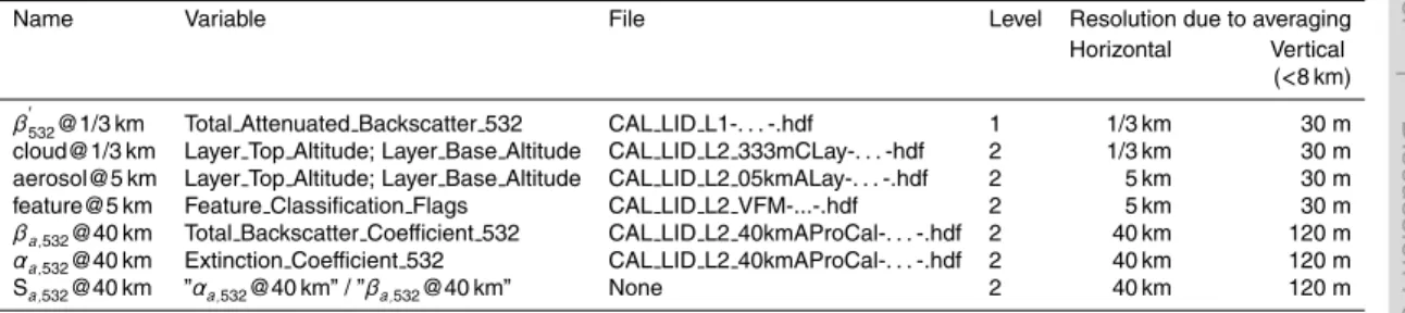
The difference between the CALIOP “curtain scenes” shown in Fig. 4a and b re-flects an additional cloud-screening of the data. Yost et al. (2008) compared MODIS 10

images overlaid with the CALIOP cloud@1/3 km product (detected and reported at a 1/3 km resolution), and the feature@5 km product (detected at all resolutions and re-ported at 5 km). It was shown that the CALIOP 1/3- km detection results are entirely consistent with the MODIS image. However, in regions populated by broken boundary layer clouds, layers detected at coarser resolutions (1- km and above) are frequently 15

misclassified as cloud. This was determined to be strictly a coding error in the cloud-clearing procedure, and not related to the algorithm design. To circumvent this error, in this part of our study, an additional cloud screening has been applied to all CALIOP β

′

532@1/3 km profiles using the cloud@1/3 km product: all CALIOPβ

′

532@1/3 km coeffi -cients are deleted underneath the highest detected cloud in the cloud@1/3 km product. 20

The black circle on Fig. 4a, b and c points out a region of the “curtain scene” showing strong initial rawβ₅₃₂′ @1/3 km coefficient values around 2.2 km on the vertical (Fig. 4a). This signal is classified as a cloud in the cloud@1/3 km product and is removed on Fig. 4b, thanks to the additional cloud screening described above. Figure 4c reports a lack of HSRL data in the corresponding region, most probably due to the presence of 25

clouds as well (the HSRL data are cloud-screened, see Table 2).

(19)

ACPD

10, 27967–28015, 2010

product

Title Page

Tables Figures

◭ ◮

Back Close

Full Screen / Esc

Discussion

P

a

per

|

Dis

cussion

P

a

per

|

Discussion

P

a

per

|

Discussio

n

P

a

per

|

section (Fig. 4c), which makes it harder to analyze in terms of potential atmospheric vertical composition. On the other hand, Fig. 4c seems to show two fairly separate and spatially homogeneous stronger regions in theβ₅₃₂′ intensity on the vertical: the lowest one lies roughly between 1 and 2 km and the uppermost one is around 3 km. In addition, the closest point to CATZ-Sanders on the HSRL track (black dashed line on 5

Fig. 4c) seems fairly representative of the rest of the 40 km “curtain scene”. Figure 5a shows the closest CALIOP and HSRLβ

′

532profile to CATZ-Sanders (black dashed line on Fig. 4b and c). Both CALIOP (Fig. 5a, blue) and HSRL (Fig. 5a, red) profiles are shown at a∼4/3 km resolution (output resolution of the HSRL subset file

and selection of the closest CALIOP profile in the 4/3 km-resolution “curtain scene” of 10

Fig. 4b). The CALIOPβ′₅₃₂profile still clearly shows a low SNR compared to the HSRL β

′

532profile.

CALIOP’s low SNR (as shown on Figs. 4b and 5a), especially in daytime, requires the spatial averaging of the attenuated backscatter profile over a significant horizontal distance to detect potential features. This is one of the tasks of the Selective Iterated 15

BoundarY Locator (SIBYL) in CALIOP’s automated level 2 product routine (Vaughan et al., 2009). In short, SIBYL consists of an algorithm that iteratively averages profiles at different horizontal scales (5, 20 or 80 km), scans those averaged profiles to detect aerosol and cloud layers, and removes detected layers from the profiles before further averaging. As a result, strongly scattering layers and portions of layers are detected at 20

finer spatial resolution, while more tenuous regions are detected at coarser resolutions. All layers detected are then classified according to type and subtype (Liu et al., 2009; Omar et al., 2009). Particulate backscatter and extinction coefficients are then de-rived for each layer detected at the 5- km, 20- km, and 80- km averaging interval, using profiles ofβ’(z) averaged horizontally to the spatial resolution at which the layer was 25

(20)

ACPD

10, 27967–28015, 2010

product

Title Page

Tables Figures

◭ ◮

Back Close

Full Screen / Esc

Discussion

P

a

per

|

Dis

cussion

P

a

per

|

Discussion

P

a

per

|

Discussio

n

P

a

per

|

final resolution of 40 km horizontal and 120 m vertical (Table 1).

The closestβa,532@40 km profile to CATZ-Sanders is shown in Fig. 5b (black), along with the collocated HSRLβ_a,₅₃₂profile (red). Unlike the processing of CALIOP profiles, we saw no necessity to average the HSRL profiles on a similar horizontal distance at the ground because of HSRL’s considerably higher SNR and accuracy. Figure 4c 5

supports this decision by showing a spatially uniform atmospheric “curtain scene” in the vicinity of CATZ-Sanders. In addition, the HSRL would cover 40 km in a few minutes (HSRL flies at ∼117 m/s) compared to a few seconds for CALIOP (flies at ∼7 km/s),

adding potential temporal di_fferences in the HSRL-CALIOP comparison.

In Fig. 5b, although the CALIOP β_a,₅₃₂@40 km profile reports no aerosol above 10

∼3.2 km or below∼1.4 km, both CALIOPβ_a,₅₃₂@40 km and HSRLβ_a,₅₃₂profiles seem

to show mostly two intensity peaks on the vertical. The change in intensity between the uppermost and the lowest peak could be due to either a change in the particle type (size and shape, hence di_fferent aerosol cross section and phase function) and/ or a change in the particle concentration and does not necessarily show two separate 15

aerosol layers on the vertical. Concerning the uppermost aerosol peak, the HSRL and CALIOP signals compare fairly well between 2.3 and 3.2 km. The standard CALIOP 5-km aerosol products (aerosol@5 km, Table 1) locate this layer (detected at a hor-izontal averaging of 20 km) between 2.7 and 3.1 km, and define it as polluted dust aerosol particles (CALIOP model S_a=65 sr). The lowest intensity peak consists of a 20

fairly constant portion of the HSRLβa,532profile recording roughly 0.003 km

−1

sr−1from the lowest few hundred meters close to the ground up to 1.9 km. Although the corre-sponding CALIOP profile starts around 1.4 km and misses a lot of the aerosol signal observed by the HSRL, it seems to pick up the lowest peak with an overestimation of 1×10−3km−1sr−1 at 1.9 km before a maximum of 5.9×10−3sr−1km−1 at 2.2 km. 25

(21)

ACPD

10, 27967–28015, 2010

product

Title Page

Tables Figures

◭ ◮

Back Close

Full Screen / Esc

Discussion

P

a

per

|

Dis

cussion

P

a

per

|

Discussion

P

a

per

|

Discussio

n

P

a

per

|

of Sect. 4.1. Indeed, the optical and microphysical properties of the aerosol plume over CATZ-Sanders tend to show a predominance of fine and strong light absorbing particles, possibly coming from a mix of haze and biomass burning particles.

In summary, Fig. 5b shows fairly good agreement between the HSRL βa,532 and CALIOPβa,532@40 km profiles, except for a lack of CALIOP values below∼1.4 km and 5

a strong peak in the CALIOPβ_a,₅₃₂signal around 2.2 km. The immediate reasons could be that (i) CALIOP, with its low SNR, cannot detect tenuous aerosol layers or reach all the way down to the lidar-detected surface due to aerosol attenuation and ii) there is a significant bug in the cloud-screening algorithm, that could explain the disparity between CALIOP and HSRLβ_a,₅₃₂around 2.2 km (corresponding to the height at which 10

a cloud is reported in Fig. 4a).

Figure 5c compares the CALIOP S_a,₅₃₂@40 km profile (=α_a,₅₃₂@40 km/β_a,₅₃₂@40 km, Table 1) with the measured HSRL S_a,₅₃₂ profile (see Table 2). For HSRL, S_a,₅₃₂(z) is simply the ratio of αa,532(z) and βa,532(z), where both quantities are measured directly by the instrument. The CALIOP retrieval 15

algorithm does not assume a profile of S_a values but assumes, instead, a single S_a value for each detected aerosol layer on the vertical. The fact that the S_a,₅₃₂@40 km profile on Fig. 5c varies on the vertical is due to the averaging of di_fferent types of aerosols that were detected at different horizontal scales. Although CALIOP and HSRL show similar averaged S_a values in the vertical (66 sr for CALIOP compared to 20

64 sr for the HSRL), CALIOP shows a much smaller range of S_a,₅₃₂@40 km (from 56 to 70 sr) compared to the HSRL (from 29 to 83 sr). The reason is that the variety of di_fferent S_a value assumptions in the CALIOP automated algorithm is much smaller than in reality. This observation leads to the introduction of a third potential explanation in the discrepancies between CALIOP and the HSRL extinction observations: iii) the 25

(22)

ACPD

10, 27967–28015, 2010

product

Title Page

Tables Figures

◭ ◮

Back Close

Full Screen / Esc

Discussion

P

a

per

|

Dis

cussion

P

a

per

|

Discussion

P

a

per

|

Discussio

n

P

a

per

|

period (i.e. measurements of S_a,₅₃₂along the CALIOP track over a large seasonal and spatial range).

The small variation of the CALIOP S_a,₅₃₂@40 km profile in Fig. 5c explains the strong resemblance of the CALIOPβa,532@40 km and αa,532@40 km profiles in Fig. 5b and d. The HSRLαa,532profile in Fig. 5d clearly shows an increase in the extinction coeffi -5

cient values between 2.4 and 3 km, followed by a stronger peak extending from∼2 km down to a few hundred meters close to the ground. On the other hand, the CALIOP αa,532@40 km profile reports the uppermost increase higher than for the HSRL with an approximate difference of 500 m on the vertical and seems to pick up∼500 m of the lowest aerosol peak (between 1.4 and 1.9 km).

10

To summarize, there are several important dissimilarities between the CALIOP and the HSRL extinction coefficient profiles on 4 August 2007. The potential reasons for those discrepancies are investigated in the remainder of this study.

4.3.1 CALIOP’s failed detection of tenuous aerosol layers and its signal not reaching down to the ground

15

We attempt to estimate the impact of failed detection of low-level aerosol layers due to high signal attenuation on column AOD, using the collocated HSRLα_a,₅₃₂profile of Fig. 5d (red). The integration of the HSRLαa,532profile from the ground to the base of the lowest layer detected by CALIOP (leading to an AOD of 0.23 from a few hundred meters to 1.5 km), and again beginning above the top of the highest layer detected 20

by CALIOP (AOD of 0.01 from 3 km to the top) adds a total of 0.24 to the standard CALIOP AOD of 0.32. Another option is to use the collocated HSRL layer aerosol optical thickness parameter, AODL₅₃₂ (Table 2) instead of the HSRL α_a,₅₃₂ profile, as AODL₅₃₂is reported from further down close to the ground (∼60 m), using the molecular

channel. The HSRL AODL₅₃₂ reports a slightly higher AOD value of 0.26 from the 25

(23)

ACPD

10, 27967–28015, 2010

product

Title Page

Tables Figures

◭ ◮

Back Close

Full Screen / Esc

Discussion

P

a

per

|

Dis

cussion

P

a

per

|

Discussion

P

a

per

|

Discussio

n

P

a

per

|

needed for CALIOP to be consistent with the AERONET AOD range 1/2 h around the overpass (0.48 to 0.73) on 4 August 2007. Based on the comparisons shown in Fig. 1, we speculate that this is not a problem specific to this case. Indeed, the CALIOP team has developed an alternative retrieval philosophy for low-lying aerosol layers. In those cases where transparent aerosol layers are detected, if (a) the initial estimate of layer 5

base is “close to” the Earth’s surface, and (b) the surface is reliably detected, and (c) the mean attenuated backscatter between the initial base estimate and the surface is positive, the layer base estimate is revised downward to a new, lower altitude very near the surface. This new scheme has been implemented in version 3 data products, and preliminary results suggest that it will have the desired effects (Vaughan et al., 2010). 10

4.3.2 CALIOP’s potentially erroneous assumed lidar extinction-to-backscatter ratio value per detected aerosol layer

An alternative CALIOPα_a,₅₃₂@40 km∗ profile was computed by applying a newly de-vised extinction retrieval to all previously cloud-screened CALIOPβ

′

532@1/3 km profiles in the 40 km region of interest (such as shown on Fig. 4b with a∼4/3 km horizontal

res-15

olution). The alternative extinction retrieval uses a simple iterative numerical method, starting from a height z₀(here, ∼4 km) down to the ground. The aerosol extinction

co-e_fficient is assumed equal to zero at heightz₀, the molecular extinction and backscatter coefficient profiles are taken from the GEOS-5 model provided in the CALIOP level 1 data, and the S_a,₅₃₂ profile is taken from the closest HSRL profile to CATZ-Sanders 20

(Fig. 5c, red). Additional information on the alternative extinction retrieval is given in the Appendix A. The alternative CALIOP AOD values along the 40 km segment are then obtained by integrating each alternative extinction coefficient profile in the “curtain scene” between∼1.4 km and ∼3.2 km, range of CALIOP detected aerosol layers and

extent of the standard CALIOPα_a,₅₃₂@40 km profile on Fig. 5d (black). The result is 25

(24)

ap-ACPD

10, 27967–28015, 2010

product

Title Page

Tables Figures

◭ ◮

Back Close

Full Screen / Esc

Discussion

P

a

per

|

Dis

cussion

P

a

per

|

Discussion

P

a

per

|

Discussio

n

P

a

per

|

pears that, in this case study, modifying the extinction-to-backscatter lidar ratio profile in the CALIOP extinction retrieval has less of an e_ffect on the final AOD retrieval (adds 0.12 in the AOD) than the impact of failed detection of low-level aerosol layers due to high signal attenuation (adds 0.27 in the AOD, previous section). The conclusion of a minor impact of CALIOP’s potentially erroneous assumed S_a value compared to the 5

inability of its signal to reach all the way down to the surface on the AOD retrieval can not yet be stated in a general context. This result may, indeed, be strongly influenced by very similar averaged HSRL and CALIOP S_a values (Fig. 5c) on 04 August 2007 close to CATZ-Sanders.

4.3.3 CALIOP’s cloud clearing, averaging and calibration of the attenuated 10

backscatter coefficient profile

Figure 6 shows the closest HSRL β

′

532profile (red) to CATZ-Sanders on 04 Au-gust 2007, along with three alternative CALIOP β′₅₃₂ profiles. The first one, called β

′ C

532,ncs@40 km

∗

(in blue on Fig. 6), is obtained by applying a sliding average of four β₅₃₂′ @1/3 km profiles before averaging all valid profiles in the 40 km segment close 15

to CATZ-Sanders (white line on Fig. 3a). The second one, called β

′ C

532,cs@40 km

∗

(in green on Fig. 6), corresponds to the first one, but with a sliding average of four profiles on the cloud-screenedβ

′

532@1/3 km “curtain scene” (Fig. 4b).

We note that the first two alternative CALIOP profiles (blue and green, Fig. 6) show more general variability than the HSRL β

′ H

532 profile (red, Fig. 6), illustrating the dif-20

ferences in SNR between the two instruments, and emphasizing the utility of using a broader horizontal averaging scale of 80 km as the input of CALIOP’s standard multi-scale averaging engine and feature detection algorithm. In addition, the comparison between CALIOP β

′ C

532,ncs@40 km

∗

(blue) and β

′ C

532,cs@40 km

∗

(green) confirms the presence of a reported cloud in the 40 km of interest around 2.2 km in height, that 25

(25)

ACPD

10, 27967–28015, 2010

product

Title Page

Tables Figures

◭ ◮

Back Close

Full Screen / Esc

Discussion

P

a

per

|

Dis

cussion

P

a

per

|

Discussion

P

a

per

|

Discussio

n

P

a

per

|

the level 2 extinction retrieval algorithm.

Two major factors need to be considered when comparing the HSRLβ

′ H

532(red) and the CALIOP β₅₃₂′C _,_cs@40 km∗ (green) profiles. First of all, the instruments differ re-garding their calibration technique and accuracy. The accuracy of the CALIOP level 1 products (and, by consequence, many of the level 2 products) critically depends on 5

the accuracy of the calibration of the attenuated backscatter profiles. The nighttime CALIOP 532 nm parallel attenuated backscatter measurement is calibrated by deter-mining the ratio between the measured signal and the total backscatter estimated from an atmospheric scattering model (Powell et al., 2009; Hostetler et al., 2006; Russell et al., 1979) across a range altitude of 30–34 km, where aerosol loading is assumed to 10

be low and there is still su_fficient molecular backscatter to produce a robust signal. Be-cause of the degradation of the SNR in the calibration region due to noise associated with solar background signals, the CALIOP daytime 532 nm calibration coefficients are interpolated from the adjacent nighttime data segments (Powell et al., 2010). On the other hand, the Airborne HSRL is internally calibrated to a high accuracy (∼1–2%), 15

and does not rely on normalization to estimated backscatter from assumed clear-air regions for calibration (Hair et al., 2008).

Secondly, the HSRLβ′H₅₃₂(red) and CALIOPβ₅₃₂′C _,_cs@40 km∗(green) profiles differ in terms of the atmospheric attenuation of each lidar signal. The attenuation of the CALIOP profile is measured relative to the base of CALIOP’s molecular normalization 20

(26)

ACPD

10, 27967–28015, 2010

product

Title Page

Tables Figures

◭ ◮

Back Close

Full Screen / Esc

Discussion

P

a

per

|

Dis

cussion

P

a

per

|

Discussion

P

a

per

|

Discussio

n

P

a

per

|

For those cases where there are no clouds above the HSRL, the magnitudes of the attenuated backscatter profiles measured by the two instruments will di_ffer by a factor of

∆T2=exp −2 ZZ_HSRL

30km

α_m(z)+α_O₃(z)d z !

(3)

so that 5

β₅₃₂′C _,_cs@40km∗

(z)_{= ∆}T2β′₅₃₂H (z) (4)

Aerosol loading is considered negligible between 30-km and z_HSRL, and thus no aerosol attenuation term is included in the calculation of_∆T2. The requisite values forαO₃(z)

andα_m(z) are estimated using the gridded ozone and molecular number density pro-file data from the GEOS-5 analysis product available from the NASA Goddard Global 10

Modeling and Assimilation O_ffice (GMAO).

∆T2 for the β′₅₃₂C _,_cs@40 km∗ profile of Fig. 6 is 0.88 (molecular and ozone optical depth are respectively∼0.04 and ∼0.02). Hence, if the CALIOP signal was correctly

calibrated, HSRLβ₅₃₂′H (red) would be∼12% higher than the CALIOPβ ′

C

532,cs@40 km

∗

(green) profile. Figure 6 shows, in fact, a general overestimation of the HSRL β

′ H

532 15

profile (red), especially along the uppermost and lowest intensity peak. We have com-puted the di_fference between the integrated red and green profiles of Fig. 6 as follows: Zz=z_HSRL

z=0km

β′₅₃₂H d z−

Zz_HSRL

z=0km

β₅₃₂′C _,_cs@40km∗

d z

×100÷

Zz_HSRL

z=0km

β₅₃₂′H d z=13.74% (5)

The amount of overestimation of the integrated HSRLβ₅₃₂′H on the integrated CALIOP β

′ C