CALIPSO observations of stratospheric aerosols: a preliminary assessment

(1)

ACPD

7, 5595–5615, 2007

CALIPSO observations of

stratospheric aerosols

L. W. Thomason et al.

Title Page

Abstract Introduction

Conclusions References

Tables Figures

◭ ◮

Back Close

Full Screen / Esc

Printer-friendly Version

Interactive Discussion Atmos. Chem. Phys. Discuss., 7, 5595–5615, 2007

www.atmos-chem-phys-discuss.net/7/5595/2007/ © Author(s) 2007. This work is licensed

under a Creative Commons License.

Atmospheric Chemistry and Physics Discussions

CALIPSO observations of stratospheric

aerosols: a preliminary assessment

L. W. Thomason, M. C. Pitts, and D. M. Winker

NASA Langley Research Center, Hampton, VA, USA

Received: 29 March 2007 – Accepted: 13 April 2007 – Published: 26 April 2007

Correspondence to: L. W. Thomason (l.w.thomason@nasa.gov)

(2)

ACPD

7, 5595–5615, 2007

Title Page

Tables Figures

◭ ◮

Back Close

Full Screen / Esc

Interactive Discussion

Abstract

We have examined the 532-nm aerosol backscatter coefficient measurements by the Cloud-Aerosol Lidar and Infrared Pathfinder Satellite Observations (CALIPSO) for their use in the observation of stratospheric aerosol. CALIPSO makes observations that span from 82◦_{S to 82}◦_{N each day and, for each profile, backscatter coe}

fficient values

5

reported up to ∼40 km. The possibility of using CALIPSO for stratospheric aerosol

observations is demonstrated by the clear observation of the 20 May 2006 eruption of Montserrat in the earliest CALIPSO data in early June as well as by observations showing the 7 October 2006 eruption of Tavurvur (Rabaul). However, the very low aerosol loading within the stratosphere makes routine observations of the stratospheric

10

aerosol far more di_fficult than relatively dense volcanic plumes. Nonetheless, we found that averaging a complete days worth of nighttime only data into 5-deg latitude by 1-km vertical bins reveals a stratospheric aerosol layer centered near an altitude of 20 km, the clean wintertime polar vortices, and a small maximum in the lower tropical stratosphere. However, the derived values are clearly too small and often negative in

15

much of the stratosphere. The data can be significantly improved by increasing the measured backscatter (molecular and aerosol) by approximately 5% suggesting that the current method of calibrating to a pure molecular atmosphere at 30 km is most likely the source of the low values.

1 Introduction

20

Aerosol plays a significant role in the chemistry and dynamics of the lower stratosphere and upper troposphere including a critical role in the heterogeneous processes that lead to ozone destruction. Stratospheric aerosol is also highly variable due to episodic volcanic eruptions that inject aerosol and/or its gaseous precursors into the strato-sphere. Over the last 25 years, the total aerosol loading has varied by more than a

25

factor of one hundred and volcanic e_ffects have dominated other natural and

(3)

ACPD

7, 5595–5615, 2007

Title Page

Tables Figures

◭ ◮

Back Close

Full Screen / Esc

Interactive Discussion derived sources for stratospheric aerosol in all but the last few years when levels have

apparently reached a stable background level (Thomason and Peter, 2006). In the ab-sence of another volcanic eruption, aerosol levels may still under go significant changes over the next decade due to changes in the human-derived aerosol precursors. Global human-derived SO₂ has declined by nearly 20% since 1980 (Stern, 2003). On the

5

other hand, emissions in East Asia and China have increased dramatically over this period and are projected to continue to increase. It is believed that SO2or SO2-derived

aerosol makes it into the upper troposphere/lower stratosphere (UTLS) through en-trainment by deep convection in the tropics and, since SO2has a short lifetime in the

troposphere, emissions at low latitudes are far more likely to make it to the tropical

10

tropopause than mid-latitude emissions (Notholt et al, 2006). As a result, it is possi-ble that changes in human-derived SO2 concentration in the lower stratosphere may

produce either an increase or decrease in aerosol loading in the lower tropical strato-sphere in the coming years. Changes in aerosol in the UTLS may a_ffect the occurrence and properties of thin cirrus in this radiatively sensitive region (e.g., K ¨archer, 2002).

15

As a result, measurements of stratospheric aerosol remain important, yet global measurements by space-borne instruments are at risk due to the end of the missions of several long-lived instruments (e.g., the Stratospheric Aerosol and Gas Experiment (SAGE II/III), The Halogen Occultation Experiment (HALOE), and the Polar Ozone and Aerosol Measurement (POAM III)) and instrument performance issues for on-going

20

missions (the High Resolution Dynamics Limb Sounder or HIRDLS). Several instru-ments have the potential to produce stratospheric aerosol data products but have yet to produce them operationally (e.g., SCIAMACHY, ACE-FTS, and MAESTRO). In light of this, we examine the Cloud-Aerosol Lidar and Infrared Pathfinder Satellite Obser-vations’ (CALIPSO) Cloud-Aerosol Lidar with Orthogonal Polarization (CALIOP) lidar

25

backscatter coefficient profiles at 532 nm as a potential source of a scientifically useful stratospheric aerosol product. While we concede that this is challenging, our prelimi-nary study (explained in detail below) suggests that a scientifically viable data product is possible even for the very low aerosol loading period currently observed.

(4)

ACPD

7, 5595–5615, 2007

Title Page

Tables Figures

◭ ◮

Back Close

Full Screen / Esc

2 CALIPSO stratospheric aerosol measurements

2.1 Description of CALIPSO

The primary objective of CALIPSO is to provide measurements that will significantly improve our understanding of the effects of aerosols and clouds on the climate system (Winker et al., 20071). As part of the Aqua satellite constellation that includes the Aqua,

5

CloudSat, Aura, and PARASOL satellites, CALIPSO is in a 98◦ _{inclination orbit with an} altitude of 705 km that provides daily global maps of the distribution of aerosol and clouds. The CALIPSO payload consists of three instruments: the Cloud-Aerosol Li-dar with Orthogonal Polarization (CALIOP), an Imaging Infrared Radiometer (IIR), and a moderate spatial resolution Wide Field-of-view Camera (WFC). CALIOP provides

10

profiles of backscatter at 532 and 1064 nm, as well as two orthogonal (parallel and per-pendicular) polarization components at 532 nm. CALIOP instrument characteristic are shown in Table 1 and the vertical and horizontal resolution of the data products is shown in Table 2. A detailed discussion of CALIOP data products can be found in Vaughan et al. (2004). In the routine processing, the parallel component of the 532-nm backscatter

15

is calibrated to the expected molecular volume backscatter coefficient between 30 and 34 km altitude where the molecular density is derived from the GEOS-4 atmospheric analyses provided by the Global Modeling and Assimilation O_ffice. The current cali-bration algorithm does not account for possible stratospheric aerosol in the 30–34 km region, as there are currently no available independent global measurements.

Inde-20

pendent calibrations occur every 55 km of the dark side of each orbit and is smoothed using a 27-point mean (1485 km) (Hostetler et al., 2006) and interpolated onto the sun-lit side. The perpendicular component is transferred from the parallel term using an on-board optical system. The calculation of a stratospheric aerosol product is highly sensitive to the quality of this normalization and any deficiency in the calibration

rep-25

1

Winker, D. M., McGill, M., and Hunt, W. H.: Initial Performance Assessment of CALIOP, Geophys. Res. Lett., submitted, 2007.

(5)

ACPD

7, 5595–5615, 2007

Title Page

Tables Figures

◭ ◮

Back Close

Full Screen / Esc

Interactive Discussion resents the greatest obstacle to the successful production of a scientifically useable

stratospheric aerosol product.

2.2 Initial assessment

With its first observations in mid-June 2006, CALIPSO provided detail of condensed material within the stratosphere. These observations included polar stratospheric

5

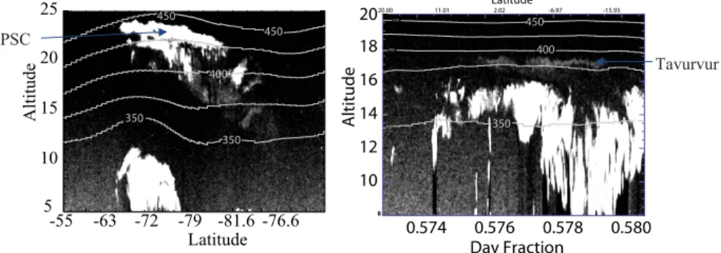
clouds (Pitts et al., 20072) as shown in Fig. 1a and a distinct aerosol plume associ-ated with the 20 May 2006 eruption of Montserrat (e.g., Carn et al., 2007). Figure 1b is an example of the observations of a second volcanic event that appeared in the lower tropical stratosphere following the 7 October 2006 eruption of Tavurvur. This plume remained clearly observable in the tropics to at least the end of November 2006.

How-10

ever, apart from these kinds of events, CALIOP backscatter data does not readily show the presence of the stratospheric aerosol layer that has been regularly measured in the past by instruments such as SAGE II and HALOE (see, for example, the browse images athttp://www-calipso.larc.nasa.gov/products/lidar/index.php).

Currently, the stratospheric aerosol column total backscatter (often referred to as

15

integrated backscatter) lies between 2 and 7×10−5str−1 at 532 nm with a peak total

backscatter to molecular only backscatter ratio (the backscatter ratio) between 1.03 and 1.06 and most of this aerosol lies within 5 to 6 km of the tropopause (Vaughan and Wareing, 2004). The integrated column back scatter is about a factor of 100 less than that following the 1991 Pinatubo eruption and also much less than what can be

ob-20

served in the boundary layer. With such low values, it is not surprising that stratospheric aerosol was not a science target of the CALIPSO mission. To establish the feasibility of producing a stratospheric 532-nm aerosol backscatter product from CALIPSO, we made use of the CALIOP data simulator developed by the CALIPSO data processing

2

Pitts, M. C., Thomason, L. W., and Poole, L. R.: Characterizations of polar stratospheric clouds by the CALIPSO spaceborne lidar: The 2006 Antarctic season, Atmos. Chem. Phys. Discuss., submitted, 2007.

(6)

ACPD

7, 5595–5615, 2007

Title Page

Tables Figures

◭ ◮

Back Close

Full Screen / Esc

Interactive Discussion team (Powell et al., 2002). This simulator includes all known sources of measurement

error including shot noise and electronic performance. As input we used a column total of 6×10−5str−1at 532 nm that corresponds to ground-based lidar measurements and,

based on a 1020-nm extinction coefficient to 532-nm backscatter coefficient ratio of 20 str−1_{, is also consistent with the stratospheric aerosol optical depth at 525 nm}

re-5

ported by SAGE II (∼0.003). The aerosol is dispersed in a “top hat” profile over a 6 km

layer between 16 and 22 km. We then produced a 20 000-km track using the CALIPSO lidar data simulator. The output was produced at the nominal resolution reported by CALIPSO of 1 km along track and 60 m vertical resolution below 20 km and 5/3 km along track and 180 m vertical resolution above 20 km. We simulated only nighttime

10

measurements in light of the low backscatter levels and noting that nighttime measure-ments are a much higher signal-to-noise ratio than daytime measuremeasure-ments.

Figure 2a shows 100 individual profiles of this data between 14 and 30 km. Other than the change in resolution (see Table 2) at 20 km, there are no obvious features in this figure and the aerosol layer is invisible. The abrupt change in noise at 20 km is due

15

to a change in on-board smoothing and not due to any atmospheric signal. Fortunately, there is no overriding reason to produce stratospheric aerosol data at anywhere close to this resolution. The most prominent existing stratospheric aerosol measurements, SAGE II and HALOE, are made by solar occultation and provide a total of only 30 pro-files a day and have a horizontal extent of hundreds of kilometers (Thomason et al.,

20

2003). As a result, we feel that substantial averaging to produce a stratospheric product is justifiable and initial assessments of data quality support this conclusion (Winker, et al., 20071). At the same time, given the lack of operational global stratospheric aerosol measurements, averaging above and beyond that representative of current measure-ments could be justified as a mechanism to preserve stratospheric record. Figure 2b

25

shows the result of reducing the resolution to 1.5 km vertically and averaging along 15 tracks through a 5-deg latitude band (a total ground track of 7500 km) or essentially, a 1-day zonal average. At this resolution, the aerosol layer is clearly visible and the uncertainty in the mean profile is only about 1%. Realistically, while the simulator is

(7)

ACPD

7, 5595–5615, 2007

Title Page

Tables Figures

◭ ◮

Back Close

Full Screen / Esc

Interactive Discussion as realistic as possible, it no doubt is missing some components of the measurement

noise that will be observed in the real data. As a result, we recognize that it is nec-essary to explore various techniques to produce robust stratospheric aerosol profiles including along track averaging, vertical averaging, and zonal averaging.

As the initial stratospheric aerosol grid, we chose a meridianal analyses of all 14

5

nighttime orbit segments averaged in 5 degree latitude between 80◦_{S and 80}◦_{N and} 1-km altitude bins covering from 10 to 40 km. This resolution is much less fine than that reported in the standard data product files and spans several changes in horizon-tal and vertical resolutions in these files (see Table 2). The tohorizon-tal number of profiles going into the analysis is on the order of 8×105 though replication of data points to

10

account for changes in resolution reduces the e_ffective number of independent mea-sures. Nonetheless, the volume of data is significantly greater than has been previ-ously available. For instance, the daily number of profiles is almost twice as many profiles as SAGE II produced during its 21-year lifetime. The molecular backscatter term is removed using the embedded molecular density originating from GEOS-4. For

15

the initial assessment, we have not made an effort to eliminate cirrus clouds, however we have crudely accounted for the presence of PSCs by eliminating all observations where the temperature was less than 195 K and aerosol backscatter is greater than 4×10−3km−1str−1at latitudes higher than 60◦ in the winter hemisphere. In the future,

we will use more sophisticated methods including the use of additional CALIPSO

ob-20

servations such as the 532-nm perpendicular backscatter coefficient and 1064-nm total backscatter coefficient measurements to more effectively deal with the presence of all clouds. An additional fact to note is that the Level 1backscatter data product (v1.10) is the attenuated backscatter that has not been corrected for attenuation by molecules, ozone, and aerosol for the two way trip between the measurement altitude and the

25

spacecraft. As a result, the reported attenuated backscatter values will underestimate true values. However, this effect is a very small in the stratosphere where the backscat-ter values particularly above the main aerosol layer are exceedingly small. As a result, we believe that the use of attenuated backscatter is unlikely to have a significant effect

(8)

ACPD

7, 5595–5615, 2007

Title Page

Tables Figures

◭ ◮

Back Close

Full Screen / Esc

Interactive Discussion on the analysis.

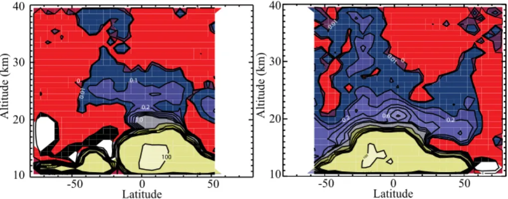
Figures 3a and b show the aerosol backscatter meridianal cross sections for 2 July 2006 and 7 January 2007. At first glance, the quality of these depictions of strato-spheric aerosol is not encouraging. While there is no evidence of the analyses being pathologically noisy, both analyses exhibit substantial areas where the meridianal

av-5

erage is less than zero and the regions that are positive are at best only somewhat consistent with expectations of how the stratospheric aerosol layer should appear. For comparison purposes, we offer a mean meridianal SAGE II aerosol extinction analysis from July 2004 as shown in Fig. 4. This is a fair comparison because SAGE II is a well-known and well-validated stratospheric aerosol data set and stratospheric aerosol

10

has been relatively constant since 2000 (e.g., Deshler et al., 2006) apart from minor effects by volcanic eruptions such as those by Montserrat and Tavurvur.

In the CALIPSO analysis, we found a persistent region in southern mid-latitudes above 25 km that is enhanced relative to other latitudes. This is most likely not a physi-cal feature and is more likely due to CALIOP instrument related effects associated with

15

the South Atlantic Anomaly. On a more positive note, in both Figs. 3a and particularly 3b, there are substantial regions that are at least reminiscent of the aerosol layer shown in Fig. 4. For a 1020-nm extinction to 532-nm backscatter ratio of 10 to 20 str (Jager and Deshler, 2002) the backscatter values range between 10−6 _{and 10}−5_km−1_str−1 and thus are somewhat lower than would be expect based on the SAGE II analysis.

20

The most robust feature in these analyses, including other days not shown, is a max-imum in backscatter coefficient between 18 and 22 km in the tropics. This is at least in part the remnant of the Montserrat and Tavurvur eruptions but may also reflect the tropical stratospheric aerosol cycle reported by SAGE II (Thomason et al., 20073).

Clearly, the current approach to calibration of the CALIOP data makes it unsuitable

25

for stratospheric aerosol analyses at current aerosol levels. The question remains,

3

Thomason, L. W., Burton, S. P., Luo, B.-P., and Peter, T.: SAGE II measurements of strato-spheric aerosol properties at non-volcanic levels, Atmos. Chem. Phys. Discuss, submitted, 2007.

(9)

ACPD

7, 5595–5615, 2007

Title Page

Tables Figures

◭ ◮

Back Close

Full Screen / Esc

Interactive Discussion however, whether improvements to the data processing and particularly the calibration

process could improve the data to a more useful state. Currently, the CALIOP data are calibrated between 30 and 34 km assuming that the atmosphere is strictly molecular including absorption by ozone or that the backscatter ratio (total to molecular backscat-ter coefficient) is 1.0 at these altitudes. This decision was based on the fact that there

5

is no routinely produced global stratospheric aerosol product available at this time. Nonetheless, based on 2004 SAGE II data, our best guess is that the backscatter ratio at these altitudes is actually at least 1.03 and possibly as large as 1.10 in the tropics (CALIOP ATDB, 2006). This discrepancy of 3 to 10% in backscatter ratio translates into a similar magnitude over-estimate of the calibration coefficient for the entire depth of

10

the profile and roughly into an underestimate of the total backscatter coefficient of the same magnitude. Since even in the main stratospheric aerosol layer, the backscatter ratio remains relatively small, the impact of the calibration overestimation may have a disproportionate effect on the measured aerosol backscatter coefficient profile.

2.3 First-order “simple” calibration fix and results

15

To evaluate the effect of the calibration issue on the stratospheric aerosol backscatter, we performed an experiment by taking the ratio of a mid-latitude northern hemisphere CALIOP meridianally-averaged 532-nm backscatter profile from July 2006 and a sim-ilar SAGE II 1020-nm extinction profile from 2004. We are relying on the belief that stratospheric aerosol loading has not changed significantly over the past two years.

20

Based on data independent of either instrument, the expected 1020-nm extinction to 532-nm backscatter ratio should lie between 10 and 20 str (J ¨ager and Deshler, 2002) as can be inferred from Fig. 5a. Figure 5b shows that the ratio profile is extremely noisy with values running between –60 and 60 str between 15 and 35 km. As a first-order cal-ibration correction, we multiply the total CALIOP 532-nm backscatter coefficient profile

25

by 1.025, 1.050, and 1.075, remove the computed molecular backscatter, and take the ratio with the SAGE II extinction profile. These profiles demonstrate substantially better behavior than the non-corrected data sets particularly below 23 km. The

(10)

ACPD

7, 5595–5615, 2007

Title Page

Tables Figures

◭ ◮

Back Close

Full Screen / Esc

Interactive Discussion corrected profile is still generally too large and varies between 15 and 45 str. On the

other hand, the 1.050 and 1.075 profiles are nearly constant around values of 8 and 15 str. The values for the 1.050-corrected profile are well within the expected range of extinction-to-backscatter values. The behavior above 23 km for all three profiles is quite similar: the extinction-to-backscatter profiles converge to values between 2 and

5

4, or significantly smaller than the nominal values. To some degree, the smaller values at higher altitudes are non unexpected as the size of aerosol generally decreases with altitude due to sedimentation and evaporation of aerosol. However, it appears that a 5% correction to the total backscatter profiles that looks promising in the 15 to 23 km range leaves backscatter too large at altitudes above 23 km.

10

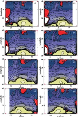
Since a 5% correction seems generally promising, we looked at monthly cross sec-tions of 532-nm aerosol backscatter coefficient for July 2006 through February 2007 as shown in Figs. 6a–h. Here we see very regular behavior in each frame that shows a stratospheric aerosol layer that stretches from about 15 km to around 22 km. There is a persistent maximum magnitude in the lower tropical stratosphere that generally

15

decreases in magnitude with time. At this point, it is not clear what the primary source of this feature is, however, it is likely that it is related either to the May 2006 Monserrat eruption or a lower tropical aerosol annual cycle that peaks in the second half of the calendar year and that has been reported previously by Thomason et al. (2006). The polar vortex measurements remain negative in this analysis. This is partly due to the

20

very low level of aerosol associated with both the northern and southern vortices and very sensitive to the quality of the meteorological data (GEOS-4) used in the data pro-cessing. Future releases of CALIOP data products will use GEOS-5 which may lead to improvement in the polar vortex analysis. The increase of backscatter coefficient in the lower stratosphere in late 2006 in the southern hemisphere is due to aerosol

origi-25

nating with the October 2006 Tavurvur eruption that appears to have been transported preferentially to southern latitudes in late 2006 in fashion similar to the 1990 eruption of Kelut (Thomason et al., 1997). The aerosol anomaly above 25 km in southern mid-latitudes is not affected by the correction. Immediately above the main aerosol layer,

(11)

ACPD

7, 5595–5615, 2007

Title Page

Tables Figures

◭ ◮

Back Close

Full Screen / Esc

Interactive Discussion the backscatter coefficient does not decrease away from the poles as would be

sug-gested by the SAGE II analysis shown in Fig. 4. It is fairly independent of latitude and, as previously noted, also appears to decrease too slowly with increasing altitude. It is possible that a simple constant correction is not adequate. This would not be surprising since the expected backscatter ratio between 30 and 34 km (and its concomitant e_ffect

5

on the calibration coefficient) is a fairly strong function of latitude. In fact, CALIOP cali-bration analyses now underway indicate the aerosol is concentrated near the equator, with maximum contributions to the 532 nm signal of about 5%.

3 Conclusions

The development of a CALIPSO stratospheric aerosol product may provide a bridge

be-10

tween current stratospheric aerosol-measuring instruments like SAGE II and HALOE and future instruments like the Ozone Mapping and Profiler Suite (OMPS). Linking these aerosol data sets is important to maintain trends but far from trivial since none of these instruments measure the same subset of aerosol optical properties and the conversion between measurement types is difficult (e.g., Thomason and Peter, 2006).

15

On the basis of this analysis, we believe that CALIPSO lidar measurements hold some promise for stratospheric applications. While it is clear that the current version does not produce stratospheric aerosol backscatter that is ready for scientific applications at current stratospheric aerosol levels, there is a clear pathway to substantial improve-ment. Future releases of the CALIOP calibration process will incorporate aerosol

cor-20

rections into the calibration process. It is possible that instruments currently in orbit may provide the needed information or a climatology based on SAGE II and/or other instruments may be adequate in the absence of significant perturbations by volcanoes. The use of GEOS-5 is expected to improve the quality of the aerosol data within the po-lar vortex (note that these concerns do not apply to observations of popo-lar stratospheric

25

clouds). Efforts to account for calibration difficulties associated with the South Atlantic Anomaly by the CALIPSO team are already underway and should also be part of the

(12)

ACPD

7, 5595–5615, 2007

Title Page

Tables Figures

◭ ◮

Back Close

Full Screen / Esc

Interactive Discussion next release of the data. It is clear that the examination of the CALIOP stratospheric

aerosol data will be useful in evaluating on-going efforts to improve operational data processing.

Acknowledgements. The authors would like to thank M. Vaughan for his helpful comments and K. Powell for performing the CALIOP simulations used in our initial study.

5

References

Bloom, S., da Silva, A. M., Bosilovich, D. Dee, Chern, J.-D., Pawson, S., Schubert, S., Sienkiewicz, M., ,Stajner, I., Tan, W.-W., and Wu, M.-L.: Documentation and Validation of the Goddard Earth Observing System (GEOS) Data Assimilation System – Version 4 . Tech-nical Report Series on Global Modeling and Data Assimilation 104606, 26, 2005.

10

Carn, S. A., Krotkov, N. A., Yang, K., Hoff, R. M., Prata, A. J., Krueger, A. J., Loughlin, S. C., and Levelt, P. F.: Extended observations of volcanic SO2 and sulfate aerosol in the stratosphere, Atmos. Chem. Phys. Discuss., 7, 2857–2871, 2007,

http://www.atmos-chem-phys-discuss.net/7/2857/2007/.

Deshler, T., Anderson-Sprecher, R., Jager, H., Barnes, J., Hofmann, D. J., Clemesha, B.,

Si-15

monich, D., Osborn, M., Grainger, R. G., and Godin-Beekmann, S.: Trends in the nonvol-canic component of stratospheric aerosol over the period 1971–2004, J. Geophys. Res., 111, D01201, doi:10.1029/2005JD006089, 2006.

Hostetler, C. A., Z. Liu, J. Reagan, M. Vaughan, D. Winker, M. Osborn, W. H. Hunt, K. A. Powell, and C. Trepte: “CALIOP Algorithm Theoretical Basis Document – Part 1: Calibration

20

and Level 1 Data Products”, PC-SCI-201, NASA Langley Research Center, Hampton, VA ,available athttp://www-calipso.larc.nasa.gov/resources/project documentation.php, 2006. J ¨ager, H. and Deshler, T.: Lidar backscatter to extinction, mass and area conversions for

strato-spheric aerosols based on midlatitude balloonborne size distribution measurements, Geo-phys. Res. Lett., 29(19), 1929, doi:10.1029/2002GL015609, 2002.

25

K ¨archer, B.: Properties of subvisible cirrus clouds formed by homogeneous freezing, Atmos. Chem. Phys., 2, 161–170, 2002,

http://www.atmos-chem-phys.net/2/161/2002/.

Kent, G. S., Winkler, D. M., Osborn, M. T., and Skeens, K. M.: A model for the separation of cloud and aerosol in SAGE II occultation data, J. Geophys. Res., 98, 20 725–20 735, 1993.

30

(13)

ACPD

7, 5595–5615, 2007

Title Page

Tables Figures

◭ ◮

Back Close

Full Screen / Esc

Interactive Discussion Lin, S. J.: A “Vertically Lagrangian” Finite-Volume Dynamical Core for Global Models. Mon.

Wea. Rev., 132, 2293–2307, 2004.

Notholt, J., Luo, B.-P., Fueglistatler, S., Weisenstein, D., et al.: Influence of tropospheric SO2 emissions on particle formation and the stratospheric humidity, Geophys. Res. Lett., 32, L07810, doi:10.1029/2004GL022159, 2005.

5

Powell, K., Hunt, B., and Winker, D.: Simulations of CALIPSO Lidar Data, ILRC 2002, Quebec City, Quebec, 2002.

Stern, D. I.: Global sulfur emissions in the 1990s, Rensselaer Working Papers in Economics No. 0311, Rensselaer Polytechnic Institute, Troy, N.Y., USA, 33 pp, 2003.

Thomason, L. W., Herber, A. B., Yamanouchi, T., and Sato, K.: Arctic Study on

Tropo-10

spheric Aerosol and Radiation: Comparison of tropospheric aerosol extinction profiles measured by airborne photometer and SAGE II, Geophys. Res. Lett., 30, 1328–1331, doi:10.1029/2002GL016453, 2003.

Thomason, L. W. and Peter, T. (Eds.): Assessment of Stratospheric Aerosol Properties (ASAP), SPARC Report No. 4, WCRP-124, WMO/TD-No. 1295,http://www.atmosp.physics.

15

ca/SPARC/, February 2006.

Thomason, L. W., Poole, L. R., and Randall, C. E.: SAGE III aerosol extinction validation in the Arctic winter: comparisons with SAGE II and POAM III Atmos. Chem. Phys., 7, 1423–1433, 2007,

20

Vaughan, G. and Wareing, D. P.: Stratospheric aerosol measurements by dual polarization lidar, Atmos. Chem. Phys., 4, 2441–2447, 2004,

Vaughan, M., Young, S., Winker, D., Powell, K., Omar, A., Liu, Z., Hu, Y., and Hostetler, C.: Fully automated analysis of space-based lidar data: an overview of the CALIPSO retrieval

25

algorithms and data products. Proc. SPIE, 5575, 16–30, 2004.

(14)

ACPD

7, 5595–5615, 2007

Title Page

Tables Figures

◭ ◮

Back Close

Full Screen / Esc

Table 1.CALIOP instrument characteristics.

laser: Nd: YAG, diode-pumped, Q-switched, frequency doubled

wavelengths: 532 nm, 1064 nm

pulse energy: 110 m Joule/channel

repetition rate: 20.25 Hz

receiver telescope: 1.0 m diameter

polarization: 532 nm

footprint/FOV: 100 m/130µrad

vertical resolution: 30–60 m

horizontal resolution: 333 m

linear dynamic range: 22 bits

data rate: 316 kbps

(15)

ACPD

7, 5595–5615, 2007

Title Page

Tables Figures

◭ ◮

Back Close

Full Screen / Esc

Table 2.CALIOP spatial resolution of downlinked data.

Altitude Range (km) Horizontal Resolution (km) Vertical Resolution (m)

30.1–40.0 5.0 300

20.2–30.1 1.67 180

8.2–20.2 1. 60

–0.5–8.2 0.33 30

–2.0–0.5 0.33 300

(16)

ACPD

7, 5595–5615, 2007

Title Page

Tables Figures

◭ ◮

Back Close

Full Screen / Esc

0.574 0.576 0.578 0.580

Day Fraction 8

10 12 14 16 18 20

Altitude

8

350 350

350

400 ₄₀₀

450 ₄₅₀

20.00 11.01 2.02 -6.97 -15.95

Latitude

5 10 15 20 25

Altitude 350

400 450

450

-55 -63 -72 -79 -81.6 -76.6

Latitude

350

Tavurvur PSC

Fig. 1. CALIOP observations of (a) a PSC observed on 24 July 2006 and(b) a qualitative

depiction of the volcanic plume from the 7 October 2006 Tavurvur eruption as measured on 15 October 2007. In both frames, the solid grey lines denote potential temperature.

(17)

ACPD

7, 5595–5615, 2007

Title Page

Tables Figures

◭ ◮

Back Close

Full Screen / Esc

0.0000 0.0004 0.0008 Aerosol Backscatter (1/km-str) 10

15 20 25 30

Altitude (km)

15

Altitude (km)

25

20

0. 0.5 1.0 1.5

-0.5

Aerosol Backscatter (10-5_/km-str)

(a)

(b)

Fig. 2. (a)A depiction of 100 individual simulated CALIPSO 532-nm backscatter profiles for a

“top hat” stratospheric layer between 16 and 22 km. The abrupt change in noise at 20 km is due to a change in on-board smoothing and not due to any atmospheric signal.(b)Simulated retrieval of a stratospheric aerosol layer using CALIPSO backscatter data. This profile is a 1-day, 5-deg latitudinal average for background conditions.

(18)

ACPD

7, 5595–5615, 2007

Title Page Abstract Introduction Conclusions References Tables Figures ◭ ◮ ◭ ◮ Back Close

Full Screen / Esc

-50 0 50

Latitude 10 20 30 40 Altitude (km) 0 0 0 0 0 0 0 0 • 1 0 1 • 1-2 1•10 -2 -2 1•10 -2 0 1 • 0 1 • 2 -1 2•10 -1 0 1 • 0 1 • 6-1 6•10 -1 0 1 1•100 1•10 0 0 4•100 8•100 0 0 0 0 0 0 0 0 0 0 0 0 0 1•1 0 -2 0 1 • 1-2 1•10-2 0 1 • 2-1 6•10 4•10 0 8•10 0 8•10 100

-50 0 50

Latitude 10

20 30 40

Altitude (km) 0.2 0.6 0.2

0.01 0 0.01 0 0.01 0.1 0.2 1.0 100

Fig. 3.CALIPSO stratospheric 532-nm aerosol backscatter profiles for(a)2 July 2006 and(b)7

January 2007. Red regions have aerosol backscatter less than zero, while white areas showing missing values. The contour values are 0, 0.001, 0.01, 0.1, 0.2, 0.4, 0.6, 0.8, 1, 2, 4, 6, 8, 10, and 100 for aerosol backscatter coe_fficient in km−1_str−1 _{times 10}5_{. Areas in the troposphere}

with extinction coefficient values greater than 10−4 km−1

str−1

are strongly influenced by the presence of cloud.

(19)

ACPD

7, 5595–5615, 2007

Title Page

Tables Figures

◭ ◮

Back Close

Full Screen / Esc

1020 nm Extinction (log10 1/km); Date: 2004/ 7

-50 0 50

Latitude 5

10 15 20 25 30 35

Altitude (km)

-6.0 -6.0

-5.0 -5.0

-4.0

-3.0

Fig. 4. Cross section of 1020-nm aerosol extinction for July 2004 as measured by the solar

occultation instrument SAGE II (in km−1 _{in log}

10). The “+” signs denote the mean tropopause height. This analysis has been had events influenced by cloud removed using the method developed by Kent et al. (1993).

(20)

ACPD

7, 5595–5615, 2007

Title Page

Tables Figures

◭ ◮

Back Close

Full Screen / Esc

2.0

1.5

1.0

0.5

0

Backscatt

er t

o

Ex

tinc

tion Kernel R

a

tio

0 0.1 0.2 0.3 0.4

Radius (µm)

1064-nm Backscatter to 1020-nm Extinction 532-nm Backscatter to 1020-nm Extinction

0.5 -60 -40 -20 0 20 40 60

Extinction-to-Backscatter Ratio 15

20 25 30 35

Altitude

(a) (b)

Fig. 5. (a)The ratio of 1020-nm aerosol extinction to 532-nm aerosol backscatter (solid) and the

ratio of 1020-nm aerosol extinction to 1064-nm aerosol backscatter as a function of radius for spherical sulfate aerosol at stratospheric temperatures.(b)Ratio of SAGE II 1020-nm aerosol extinction in northern mid-latitudes in July 2004 to the 532-nm CALIOP aerosol backscatter where the total CALIOP backscatter has been adjusted by a factor of 1 (solid), 1.025 (dotted), 1.050 (dashed), and 1.075 (dot-dash).

(21)

ACPD

7, 5595–5615, 2007

Title Page Abstract Introduction Conclusions References Tables Figures ◭ ◮ ◭ ◮ Back Close

Full Screen / Esc

-50 0 50

Latitude 10 20 30 40 Longitude 0 10 20 30 40 Longitude 0 0 0 0 0 0 0 0 1 • 1 2-1•10-2 1•10 -2 1•10 -2 0 1 • 2 1-2•10 -1 2•10-1 2•10-1 2•1 0-1 0 1 • 6 1-6•10-1 6•10 -1 6•10 -1 6•10 -1 0 1 • 10 1•10 0 1•100 0 1 • 40 4•100 4•10 0 0 1 • 80 8•100 8•100 1•1 02 10 20 30 40 Longitude 10 20 30 40 Longitude 0 0 0 0 0 0 0 1 • 1 2-1•10 -2 1•10 -2 0 1•

1-2

0 1 • 2 1-0 1 •

2-1

2•10 -1 2•10 -1 2•10 -1 6•10-1 6•10-1 6•10-1 6•10 -1 0 1 • 10 1•100 1•10 0 4•100 4•100 4•10 0 8•100 8•100 8•10 0 1•10 2 10 20 30 40 Longitude 10 20 30 40 Longitude 0 0 0 0 1 • 1 2-0 1 • 1 2-1•10 -2 1•10-2 1•10-2 0 1 • 2 1-0 1•

2-1

2•10 -1 2•10 -1 0 1 • 6 1-0 1 • 6-1 6•10 -1 6•10 -1 6•10 -1 0 1 • 10 1•100 1•10 0 1•100 4•100 4•100 4•10 0 8•100 8•10 0 8•100 10 20 30 40 Longitude 10 20 30 40 Longitude 0 0 0 0 0 1•10 -2 1•10 -2 1•10-2 1•10-2 1•1 0 -2 1•10-2 1•10-2 2•10-1 2•10 -1 2•10-1 2•10 -1 0 1 • 2 1-2•10 -1 6•10-1 6•10 -1 6•10-1 6•10-1 1•100 1•10 0 1•100 1•100 4•10 0 4•100 8•100 8•100 1•10 2 10 20 30 40 Longitude 10 20 30 40 Longitude 0 1•10-2 1•10-2 1•10 -2 1•10-2 1•10 -2 2•10-1 2•10 -1 0 1 • 2 1-2•10 -1 2•10-1 6•10 -1 6•10 -1 0 1•

6-1

0 1• 10 1•10 0 1•100 4•100 4•100 0 1 • 40 8•100 8•100 8•100 10 20 30 40 Longitude 10 20 30 40 Longitude 0 0 0 0 1•

1-2

1•10 -2 1•10 -2 0 1•

1-2

2•10 -1 2•10 -1 0 1 • 2 1-2•10 -1 6•10 -1 6•10 -1 0 1•

6-1

6•10 -1 1•10 0 1•10 0 1•100 1•10 0 4•10 0 4•100 4•100 8•10 0 8•100 10 20 30 40 Longitude 10 20 30 40 Longitude 0 0 0 0 1•10-2 1•10-2 1•1 0-2 1•10 -2 0 1•

1-2

2•10 -1 2•10-1 2•10 -1 2•10-1 6•10-1 6•10-1 0 1 • 6 1-1•100 1•10 0 0 1 • 10 1•10 0 4•10 0 4•100 8•10

0 8•100

1•10 2 10 20 30 40 Longitude 10 20 30 40 Longitude 0 0 0 0 0 1•10-2 1•10 -2 1•1 0-2 0 1 • 1 2-2•10 -1 2•10-1 2•1 0-1 0 1•

2-1

2•10-1 6•10-1 6•10-1 0 1• 6 1-6•10 -1 1•10 0 1•1 00 1•100 1•100

4•100 4•100

4•100 8•100 8•100 8•10 0 1•10 2

-50 0 50

Latitude0

-50 0 50

Latitude0 -50 Latitude00 50

-50 0 50

(a) (b)

(c) (d)

(e) (f)

(g) (h)

Fig. 6. Cross sections of CALIOP aerosol attenuated backscatter at 532 nm where the total

backscatter has been adjusted by+5% for(a)2 July 2006,(b)6 August 2006,(c)3 September 2006,(d) 1 October 2006, (e)5 November 2006, (f)3 December 2006, (g)7 January 2007, and(h) 4 February 2007. Red regions have aerosol backscatter less than zero, while white areas showing missing values. The contour values are 0, 0.001, 0.01, 0.1, 0.2, 0.4, 0.6, 0.8, 1, 2, 4, 6, 8, 10, and 100 for aerosol backscatter coefficient in km−1 _str−1 _{times 10}5_{. Areas}

in the troposphere with extinction coe_fficient values greater than 10−4_km−1_str−1 _{are strongly}

influenced by the presence of cloud. Areas within either winter time polar vortex, known to have very low aerosol content, are found to have backscatter coefficient values less than 0.