www.biogeosciences.net/11/3661/2014/ doi:10.5194/bg-11-3661-2014
© Author(s) 2014. CC Attribution 3.0 License.
On the potential vegetation feedbacks that enhance phosphorus
availability – insights from a process-based model linking geological
and ecological timescales
C. Buendía1,2,3, S. Arens1, T. Hickler4,5,6, S. I. Higgins6,7, P. Porada1, and A. Kleidon1
1Biospheric Theory and Modelling Group, Max Planck Institute for Biogeochemistry, Hans-Knöll Str. 10, 07745 Jena,
Germany
2Bayreuth Academy of Advanced African Studies, University of Bayreuth, Hugo-Rüdel-Str. 10, 95445 Bayreuth, Germany 3Ecological Modelling, University of Bayreuth, Dr.-Hans-Frisch-Str. 1–3, 95448 Bayreuth, Germany
4Biodiversity and Climate Research Centre (LOEWE BiK-F), Senckenberganlage 25, 60325 Frankfurt am Main, Germany 5Senckenberg Research Institute and Natural History Museum, Senckenberganlage 25, 60325 Frankfurt am Main, Germany 6Institute of Physical Geography, Goethe-University, Altenhöferallee 1, 60438 Frankfurt am Main, Germany
7Department of Botany, University of Otago, 479 Great King Street, 9016 Dunedin, New Zealand Correspondence to:C. Buendía ([email protected])
Received: 17 October 2013 – Published in Biogeosciences Discuss.: 10 December 2013 Revised: 18 May 2014 – Accepted: 6 June 2014 – Published: 9 July 2014
Abstract. In old and heavily weathered soils, the availabil-ity of P might be so small that the primary production of plants is limited. However, plants have evolved several mech-anisms to actively take up P from the soil or mine it to overcome this limitation. These mechanisms involve the ac-tive uptake of P mediated by mycorrhiza, biotic de-occlusion through root clusters, and the biotic enhancement of weath-ering through root exudation. The objective of this paper is to investigate how and where these processes contribute to alleviate P limitation on primary productivity. To do so, we propose a process-based model accounting for the major pro-cesses of the carbon, water, and P cycles including chemi-cal weathering at the global schemi-cale. Implementing P limita-tion on biomass synthesis allows the assessment of the effi-ciencies of biomass production across different ecosystems. We use simulation experiments to assess the relative impor-tance of the different uptake mechanisms to alleviate P limi-tation on biomass production. We find that active P uptake is an essential mechanism for sustaining P availability on long timescales, whereas biotic de-occlusion might serve as a buffer on timescales shorter than 10 000 yr. Although active P uptake is essential for reducing P losses by leaching, humid lowland soils reach P limitation after around 100 000 yr of soil evolution. Given the generalized modelling framework,
our model results compare reasonably with observed or inde-pendently estimated patterns and ranges of P concentrations in soils and vegetation. Furthermore, our simulations suggest that P limitation might be an important driver of biomass production efficiency (the fraction of the gross primary pro-ductivity used for biomass growth), and that vegetation on old soils has a smaller biomass production rate when P be-comes limiting. With this study, we provide a theoretical ba-sis for investigating the responses of terrestrial ecosystems to P availability linking geological and ecological timescales under different environmental settings.
1 Introduction
primary productivity in old ecosystems may be P limited (Walker and Syers, 1976; Wardle et al., 2004).
Low P input from weathering, however, does not mean that there is no P in old and strongly weathered soils. It just means that most of the P is not available for plants, be-cause it is in places that roots cannot access and/or occluded in secondary minerals originating from soil formation pro-cesses (Walker and Syers, 1976; Crews et al., 1995; Vitousek and Sanford, 1986). To overcome P limitation, plants have evolved strategies to make P available from these occluded pools and take it up more efficiently. These strategies in turn induce feedback processes between plants and soils, which ultimately lead to the enhancement of P availability (for a re-view on those strategies see Lambers et al., 2008). These feedback processes might lead to a sustained biomass pro-duction and resource acquisition (e.g. more leaves), which in turn allows for increased carbon fixation by plants and more below-ground investments, thus promoting P enhance-ment processes in the soil (DeLucia et al., 1997; Allen et al., 2003). While at the global scale these feedback mechanisms between plants and P availability in the soil determine to some extent the production and storage of biomass in ecosys-tems, they are also relevant for atmospheric C concentrations, and thus for the climate system (DeLucia et al., 1997; Zhang et al., 2011; Goll et al., 2012). If the biomass production of global vegetation is constrained by P availability, less carbon will be fixed to structural biomass, and therefore it will be easily respired and released to the atmosphere (Körner, 2006; Canadell et al., 2007). Hence P dynamics in soils and tation might be crucial for understanding the terrestrial vege-tation feedback on the global C cycle (Sardans and Peñuelas, 2012; Cernusak et al., 2013).
At the individual plant scale, C is assimilated during pho-tosynthesis and stored as carbohydrates in the plant (hereafter referred to as gross primary productivity, GPP). A proportion of the assimilated C is respired to run the metabolic machin-ery of plants (i.e. autotrophic respiration); another propor-tion is allocated to biomass producpropor-tion (BP) if other essen-tial nutrients are available; and the remaining proportion is stored as non-structural carbon (i.e. reserves such as sugars and starch) that is used to overcome unfavourable conditions in the life cycle of plants. The carbon allocated to growth and non-structural carbon is the net primary productivity (NPP).
Under P limitation, biomass production is constrained, which results in an accumulation of non-structural carbon in the plant. Some of this non-structural carbon can be transferred to the soil via root exudation (Jakobsen and Rosendahl, 1990; Körner, 2006; Bais et al., 2006) (see Fig. 1, blue box). In such cases, NPP can be substantially greater than biomass production. There are different pathways by which plants can enhance P availability through root exuda-tion. For example, (A) root exudates feed mycorrhizae that help the plant to actively take up P in dissolved forms; (B) root exudates, like citrate and oxalate (directly by the plant or mediated by soil micro-organisms) might release P occluded
atmosphericcarbon photosynthesis
+
+
+
+
rootexudates
-+
1
2
weathering +
Pde-occlusion +
Pactiveuptake + +
+
+
Negative feedback
non-structural carbon structuralcarbon
Pavailability
A
B
C
MO
TIVA
TIO
N
THIS
S
T
U
DY
P-lim itati
on
Figure 1.A conceptual diagram showing the feedback processes by which vegetation can affect P cycling in the pedosphere and the C cycle. Plants with abundant P supply can sequester carbon from the atmosphere and store it in biomass (path 1), which results in an overall negative feedback on atmospheric CO2concentrations. P-limited vegetation has a reduced capacity for producing biomass. Instead, it builds up non-structural carbon reserves that can lead to increased root exudation into the soil (path 2). Increasing root exu-dates increases soil respiration, potentially leading to(A)enhanced rock weathering;(B)P de-occlusion from the secondary minerals; or(C)more efficient P uptake by means of symbiosis with root my-corrhizae.
in secondary minerals, thus making it available for plant up-take (Banfield et al., 1999; Bais et al., 2006); (C) root ex-udation stimulates microbial activity and respiration in the soil. The increased microbial activity in turn increases the CO2concentration in the soil leading to an enhancement of
rock weathering (Berner, 1992; Taylor et al., 2009) and thus increased P availability (Lenton, 2001), even though this pro-cess works more indirectly than the other (A and B) mecha-nisms.
grossprimaryproductivity(kgCm-2a-1)
biom
as
s
p
ro
d
u
c
ti
v
ity
(kg
C
m
-2
a
-1
)
BP=0.6GPP
vegetation feedbacks
4 2
2
1
P-a
vaila
ble
P-limita tion
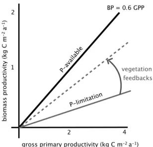
Figure 2.Theoretical relationship of P supply and biomass produc-tivity (BP) efficiency. The efficiency of BP (i.e. the slope of the line) depends on the supply of P to the ecosystem and on the degree that vegetation can enhance P availability. The maximum efficiency of BP occurs when vegetation grows under sufficient P (case 1, solid black line). In the other case, P availability limits BP (case 2, grey solid line). The carbon-energetic cost of obtaining P depends on vegetation-mediated processes within the soil: e.g. if root exuda-tions results in P gain by vegetation, then the ecosystem can produce new biomass with this biotically acquired P, which then increases BP efficiency (dotted grey line).
42 % of their total C uptake into biomass (Vicca et al., 2012). Ecosystems that are not limited by nutrients (solid black line in Fig. 2) are likely to have greater relative biomass produc-tion, which would imply a strong negative feedback on atmo-spheric CO2changes (i.e. case 1 in the blue frame of Fig. 1).
Ecosystems that are limited by P availability (or other nutri-ents), have a lower ability to produce biomass, thus resulting in a weaker vegetation feedback on atmospheric CO2
con-centrations (grey solid line in Fig. 2) unless they actively ameliorate their P limitation (grey dashed line in Fig. 2) through different processes, which also imply a C cost (red box in Fig. 1). Hence, P availability potentially constrains the biomass production efficiency of ecosystems and thereby regulates the strength of the atmospheric carbon cycle feed-back.
Understanding P availability of the world’s terrestrial ecosystems not only involves understanding P uptake but also involves understanding the pedogenetic processes (i.e. soil formation and evolution). Pedogenesis is a func-tion of time, climate, composifunc-tion of the parent material (lithology), topography, and involves the activity of the biota (e.g. soil organisms) (Jenny, 1958). Because climate, lithol-ogy and topography vary geographically across the globe, there is a great diversity of soil types and developmental stages. Additionally, catastrophic phenomena such as glacial retreats, soil removal and exposure of rock surfaces can
reini-tiate soil formation. Vegetation further affects pedogenetic processes by mediating the fluxes of carbon and water into the soil. The interaction of the different factors involved in pedogenesis ensures that soils and their phosphorus dynam-ics vary. It follows that taking into account pedogenetic pro-cesses and the propro-cesses by which vegetation can enhance P availability is necessary to understand global biomass pro-ductivity and the response of terrestrial ecosystems to the anthropogenic enhancement of atmospheric CO2
concentra-tions.
This understanding has motivated the inclusion of P lim-itation in dynamic vegetation models (Wang et al., 2007, 2010; Mercado et al., 2011; Goll et al., 2012; Yang et al., 2014). Given the complexity of these models and the small time step at which they are run they rely on P soil data and assumptions of C:N:P ratios in vegetation and soil organic
matter. This approach might work at the site scale (Runyan and D’Odorico, 2012) or in areas where P measurements exist (Mercado et al., 2011). However, at the global scale this approach is problematic given the difficultly of accu-rately measuring available P (DeLonge et al., 2013) and the high uncertainty of P maps resulting from extrapolating site-specific data on P to the global scale (Yang et al., 2013). Therefore, we take a rather simple and different approach in which only the concentration of P in different lithologies is used to initialize the model. We let the model mechanistically calculate soil formation, weathering and erosion processes, at the same time as vegetation carbon, water and phosphorus dynamics.
The aim of this study is to estimate the effect of P avail-ability on terrestrial biomass production and the extent to which vegetation can alleviate P limitation by P enhancement processes, using a process-based model that links processes working on ecological and geological timescales.
To do so, this paper is structured as follows. First, we pro-vide an introduction to our model including a detailed de-scription of the P cycle and how we implemented its different components into our C–P biogeochemical model. In doing so, we also define simulation scenarios used to determine the importance of P enhancement processes on long-term NPP and BP. Second, we introduce the criteria we used to select a model scenario from the three simulation experiments and explain how the simulations are evaluated against observa-tions. Third, the model performance with respect to the geo-graphic variation of P in the soil and C in vegetation as well as their temporal dynamics is assessed. Finally, we discuss the limitations and general applicability of our approach as well as its implications.
2 Methods
how vegetation, soil, water and carbon feedbacks influence soil formation. The model is based on the concentrations of elements in different lithological classes, topography and cli-mate and calculates chemical weathering of primary miner-als, erosion of secondary minerminer-als, and the associated tec-tonic (isostatic) uplift. This model is coupled to a simple vegetation model that is forced by daily climate (i.e. precip-itation, temperature, humidity) to calculate soil–vegetation water and carbon balances (Porada et al., 2010). Phospho-rus weathering is described as a process depending on P concentration in the different lithological classes and cal-cium weathering, which is calculated in the regolith model. The abundance of secondary minerals (clays) calculated by the regolith model determines P occlusion and erosion. The (passive) P uptake by plants depends on their water uptake. The availability of inorganic phosphate in vegetation biomass constrains photosynthesis, as without it, the transformation of energy into Adenosine triphosphate (ATP) is not possible. Synthesis of vegetation biomass requires inorganic P to form phospholipids and genetic material; without P the synthesis of metabolic active tissue is not possible. The carbohydrates that are neither respired nor synthesized into biomass accu-mulate in the plant. A fraction of these carbohydrates can be utilized as root exudates. Root exudates are rapidly respired in the soil thus altering the soil CO2balance as represented
in Fig. 1 path A. Biotic P uptake and P de-occlusion as repre-sented in Fig. 1 paths B and C also depend on root exudation but have different effects in the soil as the first only uses the P that is in the soil in available forms, and the second uses the P that is bound to secondary minerals. These processes are also included in the model and can be switched on and off allowing simulation experiments that test the relative im-portance of the three processes on the biomass production by vegetation.
2.1 Model formulation
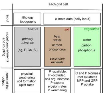
The biochemical model used here explores the short (daily) and long-term (thousand to hundred thousand years) inter-actions between the biogeochemical C and P cycles, given (fixed) lithological, topographical and climatological con-straints. The model runs on a global scale in which the fluxes of water, carbon, phosphorus and heat between the soil and vegetation are calculated on a daily time step. The model also accounts for the pools of calcium, silicates and other primary mineral fluxes in the bedrock and their export to the soil. The diagram shown in Fig. 3 summarizes the model inputs, com-partments and outputs.
The basic version of the model, which is called JESSY-SIMBA, was conceived as a simple global model of ter-restrial biogeochemistry accounting for the most important fluxes of carbon and water. This version is well documented and tested in Porada et al. (2010). An extension of JESSY-SIMBA, including soil formation, erosion and weathering, called the regolith model was documented and tested by
so me o f t h e output input mo d e l co mp a rt me n ts a n d co u p lin g
lithology climate data (daily input)
water
primary minerals
(eg, P, Ca, Si)
water
carbon carbon phosphorus
secondary minerals
C and P biomass root exudates NPP and GPP P uptake P -available,
P -occluded, soil org. biomass
P exports erosion rates P weathering physical weathering soil formation uplift rates
bedrock soil vegetation
each grid cell
topography
heat
phosphorus
Figure 3.Diagram of the model structure (after Porada et al., 2010). The model uses daily climate data, topography and lithological classes as input. It has three main components – bedrock, soil and vegetation in which fluxes of primary minerals from the bedrock are calculated. Vegetation dynamics drive water, carbon and phos-phorus dynamics. The model calculates e.g. weathering rates, gross primary productivity and biomass production. For an extensive list of the model outputs see Table A3
Arens (2013). The regolith model provides the carbon cy-cling module of the C–P model. This model was used here because it captures well the global patterns of Ca2+ and
HCO−3fluxes across climatic and tectonic gradients, which
are derived from weathering. The P model described in Buendía et al. (2010) was the basis of the P dynamics mod-ule, and it captures the general dynamics of P in pedogenesis and soil moisture effects on P dynamics. To couple C and P dynamics, a number of changes in the soil and vegetation C dynamics were necessary: (1) the carbon pool in vegetation was split into structural carbon Cvo, and storage carbon Cvc; (2) the storage carbon from vegetation flows to the soil generat-ing a new flux and pool of organic carbon in the soil Csc; (3) the inclusion of biotic de-occlusion of P resulted in a pool of carbon associated with secondary minerals (e.g. aluminium citrate) Cs
y.
Figure 4 summarizes the C and P fluxes between bedrock, soil, vegetation and atmosphere as they were considered in this model.
Pov
Pos Pdv
Pds
Pms Pys
Cov
Cos Ccv
Ccs Cgs Cys
Cga
vegetation (v)
soil (s)
bedrock (b) atmosphere (a)
(=360 ppm) phosphorus dynamics carbon dynamics
fPdov
fPovs
fPods fPmds
fPmbs fPdys fPyds
fPdsv
fCgcav
fCcov
fCovs
fCogs fCcgs
fCcgvs fCcvs
fCcys fCcgva
Figure 4.The C–P biogeochemical model: symbols in bold denote pools and symbols, in italic denote fluxes between pools. Black ar-rows show fluxes in the standard version of the model (W-P); blue arrows show P de-occlusion and the associated carbon flux to re-calcitrant forms (BD); red arrows show P active uptake mediated by mycorrhizae and its associated carbon respiration (BAU). The model has a switch for turning on and off active P uptake (blue fluxes) and biotic de-occlusion of P (red fluxes). For definition of symbols see Table A3.
formf Asabt, wherebis start andt the end state (to consider phase change) andsis the start andathe end location. P root uptake from soil to vegetation is thus namedfPsvd.
2.2 Bedrock related processes 2.2.1 Weathering
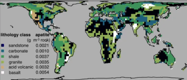
The main input of P to terrestrial ecosystems is chemi-cal weathering; therefore, an appropriate implementation of the weathering fluxes in the model is essential. To estimate weathering rates globally, tectonic uplift rates and P concen-trations in primary minerals are needed. Arens (2013) solves this problem by assuming that uplift equals erosion. The to-pographic relief is constant through simulation time, which means that there must be uplift, or else topographic relief would decline. In principle, in steady state, minerals of the bedrock constantly replace eroded material, so the weight of the soil column remains constant (on a yearly basis). Only few minerals contain P in large amounts, in igneous rocks it is present in tiny crystals in the form of fluorapatite, while in sedimentary rocks it is found associated with authigenic carbonate fluorapatite (Filippelli, 2008). P concentration is higher in igneous rocks than in sedimentary rocks. To ac-count for this differences the model uses the lithological map of Amiotte Suchet and Probst (1995) with apatite concentra-tion of primary mineral estimated from Newman (1995) see Fig. 5).
Tectonic uplift of apatite from the bedrock to soil (fPbsm) is defined as uplift rate (uplift) multiplied by the concentration
Table 1.Abbreviations of variable names. State variables are con-ventionally named Ac
b, where A is a chemical compound, e.g. P, or a state variable such as temperatureT,bis the state of matter, e.g. s for solid (see Table 1). Fluxes have names of the formfAsa
bt, where bis start andtthe end state (to consider phase change) andsis the start andathe end location. P root uptake from soil to vegetation is thus namedfPsvd. Pools start with the element, fluxes start withf, parameters withp, and constants withc.
Abbreviation
Element water H2O
phosphorus P
calcium Ca
carbon C
State solid s
liquid l
gaseous g
dissolved d
actively metabolizing biomass o
carbohydrates c
bound to primary mineral m
bound to secondary mineral y
Reservoir atmosphere a
vegetation v
soil s
river channel r
bedrock b
of apatite (pP), given by the lithology (see Fig. 5 P concen-trations and for global patterns):
fPbsm=pP(uplift). (1)
The weathering module has been already tested and docu-mented for calcium fluxes in Arens (2013). Since phosphorus in rock material is a trace mineral, we calculate P weathering as a sub-product of calcium weathering (fCapd):
fPsmd=fCapd P
s m
Cap (2)
where Ps
mand Capare the concentrations of P and Ca in
pri-mary minerals in the soil (see Appendix A5 for the balance equations). Note that calcium fluxes follow the notation pro-posed in Arens (2013) instead of the notation propro-posed in Porada et al. (2010).
2.2.2 Secondary mineral formation and P occlusion Primary rocks react with CO2and water, releasing its
sandstone carbonate shale granite acid volcanic basalt
0.0021 0.0010 0.0037 0.0035 0.0032 0.0054 lithology class apatite (g m-3 rock)
Figure 5.Map of the lithological classes and their respective ap-atite concentrations (g apap-atite m−3). Lithological classes taken from
Amiotte Suchet and Probst (1995), values for the concentration of apatite were calculated from Newman (1995).
the weathering reaction, resulting in weathering being lim-ited by the calcium export capacity of the soils, which is referred to as the ecohydrological limitation to weathering (Arens and Kleidon, 2011). Whereas on landscapes with low topographic relief, where erosion is low and therefore tec-tonic uplift as prescribed in the model is low, the limitation to weathering is the supply of new fresh primary minerals.
The increase of secondary minerals with soil formation in-creases their capacity to co-precipitate phosphate by binding P to Al, Fe, and Mn (Filippelli, 2002). This process is re-ferred to as P occlusion (fPsdy) in this model and is formu-lated as a function of secondary mineral density (Clays) and P availability in the soil (Psd):
fPsdy=pτPsydClaysPsd, (3)
wherepτPs
ydis the occlusion rate of P, bound by secondary
minerals (y), in dissolved state (d) in the soil (s). 2.3 Vegetation dynamics
In regions with sufficient P availability, passive uptake of P is sufficient to satisfy vegetation demands of P. In regions with low P availability, vegetation relies on active P uptake mechanisms. Therefore, we formulate P uptake by vegetation (fPsvd) as a combination of passive and active P uptake. Root water uptake,fH2Osvl (i.e. flow from soils (s) to vegetation
(v) in liquid form (l)), drives passive P uptake:
fPsvd =afPsvdfH2Osvl
Ps d
H2Ols. (4)
In Buendía et al. (2010), mycorrhizal hyphae were found to be very important for maintaining P in vegetation, particular-ity in old ecosystems. While accounting for carbon dynam-ics, it makes sense to associate a carbon cost with this sym-biotic P uptake mechanism between plant and mycorrhiza. Therefore, the enhancement factorafPsvd is defined as a func-tion of root exudafunc-tion of carbohydratesfCsvc of the following
form:
afPsvd =1.0+cSUtanh(pτPsvdfCvsc ), (5)
which reaches an asymptotic limit ofcSUat high exudation rates. By setting the value ofcSUto 0, the effect of active up-take can be switched off. For the simulations considering this feedback and presented here the maximum value that the en-hancement factor can take is set to 10 (cSU=10). Note that
without this carbon-mediated mechanism the implementa-tion of this value at the global scale led to unrealistic amounts of Pvd, particularly in areas with sufficient P supply.
2.3.1 Gross primary productivity (GPP)
In the original JESSY-SIMBA model, gross primary produc-tivity (GPP,fCavgc) was a simple parameterization of carbon and water fluxes, constrained by light, temperature, soil wa-ter and relative humidity (for details, see Porada et al., 2010). Here, motivated by the role that ATP plays in short-term en-ergy storage for photosynthesis, gross primary productivity (fCavgc) is further constrained by P availability, Pvd:
fCavgc=
(
min(fCav
gc[light], fCavgc[water]), Pvd>0,
0, Pvd=0.
The carbohydrates taken up during photosynthesis are par-tially respired (autotrophic respiration). Those that remain are referred to as net primary productivity (NPP). Synthesis of structural biomass occurs only when other nutrients are also available; therefore, biomass productivity equals NPP only in cases when ecosystems are not limited by other nu-trients.
2.3.2 Biomass production and net primary productivity NPP for the purpose of this study is taken as 60 % of GPP, as data suggest that a maximum of 60 % of GPP can be al-located to biomass (Vicca et al., 2012). To calculate the syn-thesis of actively metabolizing biomass (BP), first the po-tential fluxes are calculated. The popo-tential carbon flux is de-fined as NPP plus carbohydrate storage in vegetation (Cvc), thusafCvco=0.6fCavgc+Cvc while the potential P synthesis is defined as a fraction,cmaxfPdo, of inorganic phosphate in
vegetation Pvd,afPvdo=cmaxfPdoPvd. Finally, the minimum
between the potential fluxes is calculated:
fCvco=min(afCvco, cCPvafPvdo)andfPvdo=fC
v co
cCPv (6)
The minimum between the potential fluxesfCvcois the actual
biomass synthesis (or BP). In cases where C or P limits BP, the non-limiting nutrient is then stored. Carbon is stored in C-rich structural carbohydrates Cv
cand the inorganic phosphate
formulation of carbon in vegetation. That is because the leaf area index (m2leaf surface per soil surface) depends on the
biomass that contains P and not on the carbohydrate storage. Total carbon in vegetation is then the sum of structural Cv o
and storage Cv ccarbon.
2.3.3 Autotrophic respiration
In the original version of the model, the difference between GPP and NPP is denoted by autotrophic respiration fCcgv :
half was respired into the soil (fCvscg) and half into the atmo-sphere (fCvacg). Here, autotrophic respiration is divided into growth and maintenance. For each carbon unit fixed in struc-tural biomass (Cv
o), 0.25 carbon units are respired. Therefore,
growth respiration (pBPcg) is set to 0.25 (i.e.pBPcg=0.25)
(Lavigne and Ryan, 1997). Maintenance respiration is de-fined with respect to actively metabolizing biomass (Cv
o), as
follows:
fCvcg=pBPcgfCvco+Q10Cvo. (7)
Maintenance respiration depends on temperature and on the size of the structural carbon pool Cv
o, therefore theQ10
rela-tion was used:
Q10=cq10
Ts−cTMelt−10.0 10.0
pτCs
o
. (8)
TheQ10relation depends merely on soil temperatureTs. The
decay rate is given by a global constant parameterpτCsothat
is obtained by matching observations (IGBP-DIS, 1998). 2.3.4 Carbon and phosphorus losses from vegetation The input of C and P into the soil via litterfall (fCvs
o and
fPvs
o, respectively), root C exudation (fCvsc ) and leaf
leach-ing of P (fPvsd) are proportional to their respective plant pools Cv
o, Pvo, Pvdand Cvc. For litter we used the formulation of
Po-rada et al. (2010):
fCvso = C
v o
pτCv
o
for C andfPvso =fCvso P v o
Cov for P, (9)
wherepτCv
orepresents the residence time of biomass in
veg-etation. Despite the changes in carbon dynamics of the vege-tation, this parameter was not re-calibrated.
Root exudate residence time pτCv
c is not known.
How-ever, in steady state root exudation equals carbohydrate and starch formation. Therefore, the parameterpτCvc was set by personal assessment to match total carbon in vegetation:
fCvsc = C
v c
pτCvc. (10)
The losses of inorganic phosphate in vegetation (Pvd) are de-coupled from the losses of P in biomass (Pvo) – it has been observed that plants reabsorb P before dropping the leaves.
Probably they can reabsorb inorganic P used for photosyn-thesis, but not the organic P that is found in DNA or phospho-lipids. A minimal fractional loss was defined to avoid super-saturation of P of plants in regions with high P availability:
fPvsd = P
v d
pτPvd. (11)
2.4 Soil processes 2.4.1 Decomposition
Organic matter decomposition (fCsogandfPsod) is a process
mediated by soil fungi and microbes, whose rates of activity depend on soil moisture and temperature, substrate supply and nutrient availability (Davidson and Janssens, 2006). In JESSY-SIMBA decomposition depends merely on tempera-ture since that better predicts the soil organic biomass pat-terns (Gholz et al., 2000):
fCogs=CsoQ10andfPsod=fCsog
Pso Cs o
. (12)
The model assumes that carbon root exudates are respired almost entirely by mycorrhizae and soil micro-organisms (Kunc and Macura, 1966), which is expressed by the flux
pMyCcgfCvsc , where pMyCcg is a parameter that accounts
for respiration. Only small amounts of carbon root exudates reach the mineral soil, and those follow also theQ10relation
(Eq. 8). Heterotrophic respiration of root exudates is thus de-scribed as
fCscg=pMyCcgfCvsc +CscQ10. (13)
2.4.2 Biotic de-occlusion of P
In very old weathered soils, like those of western Australia, some of the plants have cluster roots instead of mycorrhiza associations (Lambers et al., 2008). Those roots produce car-boxylates (e.g. oxalate and citrate), which can replace the P that is bound to aluminium and iron, and thus release this P (Bais et al., 2006; Lambers et al., 2008). This relation re-quires one sugar (six moles C) per one exchanged P (cCPsy).
Although we do not account for the process in molecular de-tail, organic acids are respired at a very high rate, with less than 5 % reaching the mineral soil (Kunc and Macura, 1966). The remaining carbon Cs
cmight be used for P to C exchange.
Therefore, P de-occlusion is calculated as the minimum be-tween occluded P (namely Ps
y) and plant root exudates in the
soil Cs c
fPsvyd=min P
s y pdt, cCP
s y
Csc
pdt andfC ss
cy=fPsvydcCPsy. (14)
With the introduction of this process a new pool of carbon in the soil is created, which accounts for the carbon that was exchanged with P in secondary minerals (e.g. aluminium cit-rate). We refer to this pool as the recalcitrant carbon in the soil, Cv
2.4.3 P losses
Phosphorus is lost from the system by baseflowfH2Olscand
erosion (driven by topography and atmosphere). Our model accounts for baseflow losses (i.e. losses of P from percolating water) of dissolved P and erosion-caused losses of occluded P. The reasons for excluding losses of litter and organic mat-ter due to erosion and runoff are given in the discussion. For consistency the model does not consider atmospheric losses of P, because atmospheric inputs of P, via e.g. deposition of dust, are also not accounted for. This simplification will be justified in the discussion.
Baseflow losses Losses of Pv
dare driven by baseflow (described in Eq. 9,
Po-rada et al., 2010), which is proportional to the total concen-tration of P in the soil solution ( Pscd
H2Ols),
fPscd =fH2Olsc
Psc d
H2Ols. (15)
Erosion of secondary minerals and P occluded
The empirical formulation of physical erosion accounting for the denudation of secondary minerals driven by topographi-cal gradients was originally proposed in Hilley and Porder (2008) (Eq. 22, Arens, 2013). Losses of occluded P are cou-pled to the losses of secondary minerals (fClaysr) and there-fore defined as
fPsry =fClaysr P
s c
Clays. (16)
Although it is not clear what happens to the recalcitrant carbon formed in the soil (Cs
y), it is assumed that baseflow
drives the losses of this pool and of the organic acids pool Cvc,
fCsry =fH2Olsb
Csy H2Ols and
fCsrc =fH2Olsb C
s c
H2Ols
. (17)
2.5 Simulation setup 2.5.1 Climate forcing
The model was run using daily climate data from the NASA Land Surface and Hydrology archive (Sheffield et al., 2006) for the time period 1960–1989 rescaled on a global rectan-gular grid with a resolution of 2.810×2.810 long–lat degree. Daily means of temperature, precipitation, relative humidity and long-wave and short-wave radiation were used as input to model. The glacial cover of the last glacial maximum was used to define areas where regoliths are necessarily much younger than in the rest of the world. Areas that were cov-ered by glacial lakes were treated in the same way as areas that were covered by ice (Arens, 2013).
2.5.2 Simulation scenarios
Model simulations were run in low resolution (2.810×2.810 long–lat degree) for 150 000 yr. For comparison with other model estimates the model was run at a higher resolution (1.125×1.125 long–lat degree) for 70 000 yr.
Figure 6 gives an overview of the processes implemented in the model and the possible feedbacks on P availability to vegetation. We will focus on quantifying the role of (a) biot-ically active P uptake (BAU) and (b) biotic de-occlusion of P (BD). A control scenario to test the enhancement of weath-ering through root exudation (W-P) could not be defined be-cause P limitation with the proposed model structure cannot be decoupled from root exudation. Therefore, the W-P feed-back cannot be quantified, but since this approach includes root exudates which change soil respiration this feedback is included in all the simulations.
1. W-P: describes the simplest dynamics of the P model. When P is limiting the new formation of structural biomass, carbohydrates accumulate and are released as root exudates. The exudates are quickly respired in the soil. This might enhance weathering in regions where CO2 is the limitation to weathering as described in
Arens (2013). This simulation is run only for 50 thou-sand years, as the vegetation becomes very P limited.
2. BD: biotic de-occlusion of P from the occluded pool. In this simulation root exudates interacted with secondary minerals to exchange C with P as described in Eq. (14). This also includes the possible root exudates feedback on weathering. This simulation was run for 50 000 yr.
3. BAU: biotic active uptake of P from the available pool as described in Eq. (5). In this version we assessed the role of mycorrhizae in sustaining productivity at long time scales. W-P was also included. This simulation was run for 150 000 yr at low spatial resolution and for 70 000 yr at high spatial resolution.
4. BD-BAU: includes biotic de-occlusion and biotically ac-tive uptake of P. This simulation was run for 50 000 yr.
+
+
+
root symbionts +
soilCO2
+
+
+
+ +
non-structural carbon
structuralcarbon
Pavailability
W-P
P
-li
mita
ti
o
n
P-available
+
Control-P
BD-P BAU-P
weathering
Pactive
uptake
root exudates
bioticP
deocclusion
Figure 6.Diagram showing the modelled carbon feedbacks on the P availability. Simulation scenarios are defined with respect to these feedbacks. Dashed line represents the effects that can be turned off and dotted line represents the unrealistic Control-P.
2.5.3 Assessment of vegetation feedbacks on P availability
Since the carbon dynamics of the model were changed with the coupling to the P cycle, comparison of our results with the results presented in Porada et al. (2010) was not suitable. A scenario in which P dynamics were included, but the vege-tation was unlimited by P, was defined as the biomass control scenario to which all other scenarios were compared. Stand-ing biomass was calculated as 10 yr means at every 50 000 yr intervals. The scenario in which the C feedbacks on the P cy-cle could most effectively reduce P limitation (i.e. smallest difference in standing biomass to the control scenario) was selected for further simulations, using higher spatial resolu-tion.
2.5.4 Model evaluation
After comparing the different scenarios, we choose the less P-limited and closer-to-observations scenario to run the model for 70 000 yr at a high resolution (1.125×1.125 long– lat). To evaluate our model’s performance, we compared the geographical patterns of soil P pools to the data-driven model-estimated P soil pools of Yang et al. (2013), and to results of the model study of Goll et al. (2012).
For the evaluation of temporal dynamics, the model was run only until 150 000 yr because already at 40,000 years the regolith model reaches steady state (Arens, 2013). Low reso-lution (2.810×2.810 long–lat) was used to reduce the
com-putational cost. Five-year means were calculated at 10 000; 50 000; and 150 000 yr for (a) the weathering fluxes, (b) C and P in vegetation biomass, (c) gross primary productivity, (d) biomass productivity, and (e) P availability in soil solu-tion. We compared the model results with literature estimates and general insights gained from chronosequences.
3 Results
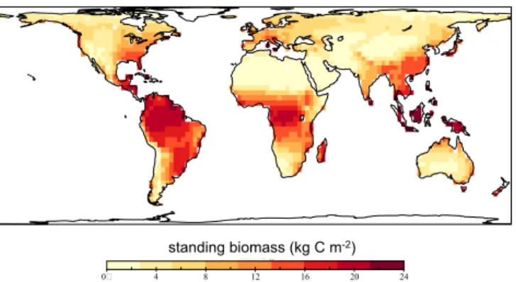
3.1 Evaluation of vegetation feedbacks on P availability The control-P scenario was defined so that P was not lim-iting photosynthesis and biomass production. In that sce-nario biomass pools reached their maximum value given the light and water constrains. Figure 7 shows the geographical biomass patterns without P limitation. The biomass reaches its maximum at about 24 kg C m−2 which is in accordance
with satellite-derived estimates of total biomass (Saatchi et al., 2011).
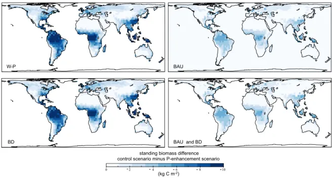
To test the importance of the processes mediated by veg-etation to enhance P availability we compare the control-P scenario with the other scenarios including gradually more processes. Figure 8 shows the differences in total vegeta-tion biomass between the control-P scenario and the other four scenarios, (BD, BAU, BD-BAU and W-P, defined in Sect. 2.5) in ecosystems after 50 000 yr of soil evolution. In general, we find less differences between the control-P and the scenarios accounting for BAU (shown in the two right panels). The simplest scenario considering only the veg-etation feedback on weathering (W-P) indicates that, after 50 000 yr, vegetation is extremely P limited worldwide (top left panel). The scenario considering both W-P and biotic de-occlusion (BD) shows a very similar limitation on standing biomass (bottom left panel). BAU shows less overall limi-tation to P compared to the scenarios not including it. The maximum absolute differences between W-P and BAU are about 10 kg C m−2.
standing biomass (kg C m-2)
Figure 7. Carbon in terrestrial vegetation biomass of the control run. In this scenario the vegetation growth is constrained only by water, light, and temperature so that vegetation biomass reaches its maximum everywhere around the globe, while not accounting for P limitation. In this simulation biomass reaches 24 kg C m−2in some
tropical areas.
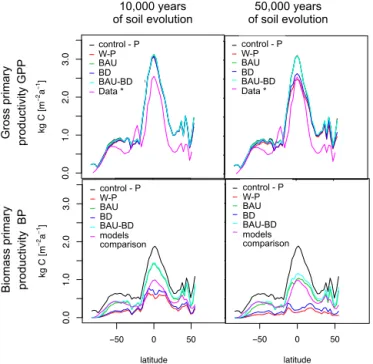
smallest differences to the control scenario are those con-sidering BAU. After 10 000 yr BAU and BAU-BD overlap, and after 50 000 yr BAU and BAU-BD decrease with the rest to 10 000 yr although BAU-BD is slightly less. The model inter-comparison for NPP from Cramer et al. (1999), which usually is interpreted as BP, is included as a reference. The scenarios including BAU best fit this line.
Overall, mycorrhizae-mediated P uptake is identified as a very important mechanism in terms of maintaining ecosys-tem biomass during longer timescales (over 50 000 yr). That is represented by the differences between right and left pan-els in Fig. 8. This process is important, not only in the tropics, but also in temperate regions. Therefore, BAU was included in further simulations. In contrast, including the P cycle with-out this carbon feedback leads to a scenario with very high limitation to biomass production. Biotic de-occlusion was in-efficient due to the lack of replenishment of the P that was oc-cluded. Simulations including this feedback led to unrealistic scenarios in which, particularly in the tropics, unrealistically low amounts of the P occluded were found at the end of the simulation.
Our previous results regarding vegetation C dynamics highlighted the importance of mycorrhizal-mediated P up-take and the inefficiency of biotic de-occlusion to supply P to old ecosystems. Regarding standing biomass patterns, the simulation including both BD and BAU imposed the small-est constraint on standing biomass. However, the difference to the scenario including just BAU was very small. The sce-narios that included the BD feedback gave unrealistic P oc-cluded ranges and global patterns. Therefore, the BAU sce-nario was run for 70 000 yr at a higher resolution to compare spatial and temporal patterns of model results with observa-tions.
3.2 Evaluation of modelled soil and vegetation P spatial patterns and temporal dynamics
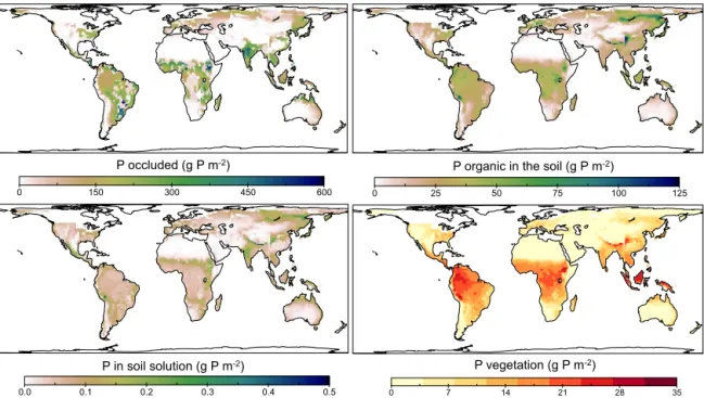
Figure 10 shows the P status of soils and vegetation after 70 000 yr of simulation. Because glaciation and volcanism restart the soil forming process and are not included in our model, our map cannot accurately reproduce present condi-tions across the globe. However, it presents general features of how climate, topography and lithology might influence soil P status and vegetation productivity. Places that were glaciated during the last glacial maximum (about 21 000 yr ago) are omitted here. Because P in primary minerals in the bedrock was also considered, the total amount of apatite is not presented here. The occluded P pool is the largest P pool in soils. Our numbers are of the order of magnitude estimated by Yang et al. (2013) and the patterns look similar (see for comparison Appendix B, Fig. B2). The second largest pool in the soil is P in litter and soil organic biomass (top-right panel). Our model estimates are five times smaller than the ones given by Yang et al. (2013) (see for comparison Ap-pendix B, Fig. B1). However, our upper range is higher than that reported for agricultural soils, 25 g P m−2 (Brady and
Weil, 2008), and in general agreement with ranges and pat-terns from Goll et al. (2012). The modelled dynamics with re-spect to P in vegetation are within the observed ranges (Brady and Weil, 2008) and also in agreement with modelled esti-mates by Goll et al. (2012) (see Fig. 2). Figure 11 shows the performance of vegetation including P dynamics. The total biomass patterns are in agreement with estimates by Saatchi et al. (2011). Although there are no big differences in the patterns of GPP and BP, the map of biomass productivity ef-ficiency, here, is the result of P limitation.
Overall, we found reasonable agreement between our modelled P global patterns and independent data- and model-based estimates, in particular considering the substantial un-certainty associated with the data sets used here for compar-ison. Figure 12 shows how weathering, carbon to phospho-rus ratio in vegetation and biomass productivity efficiency change in time. Putting those plots together enables us to see how patterns are correlated. The P weathering rates, calcu-lated from our model, are in the range of observed values (50 to 1000 g P ha−1a−1) (Newman, 1995), after 10 000, 50 000
standing biomass difference control scenario minus P-enhancement scenario
BAU W-P
BD BAU and BD
- - - -
-(kg C m-2)
Figure 8.Difference in the standing biomass of the control with the different feedback scenarios for the world after 50 000 yr of soil evolution. Biomass differences between the control simulation (see Fig. 7) and W-P (top left), BD (bottom left), BAU (top-right), BAU-BD (bottom right). W-P shows the greatest differences with the control scenario: more than 50 % biomass reduction worldwide – the differences are high in temperate coastal areas (e.g. Chile, Guyana and South Africa). BD (bottom left) shows a very similar pattern to the W-P scenario, with only small differences in temperate regions. Biotic active uptake (BAU) (top-right panel) shows much smaller differences to the control, with the absolute greatest differences located in the tropics. BAU-BD (bottom right) shows a pattern almost identical to the BAU scenario, with only very little differences.
150 000 yr serves as the best data comparison for this area. Differences in the allocation of carbon and plant character-istics between western and eastern Amazon basin have been observed (Quesada et al., 2012; Saatchi et al., 2011). Over-all, we see how the ecosystems shift towards P limitation over time. After 10 000 yr of soil formation, most of the ecosys-tems have enough P for biomass synthesis and therefore have high BP to GPP ratio (refer to left panels). However, over time (after 100 000 yr), more ecosystems shift towards P lim-itation, reducing the overall biomass productivity efficiency. 3.3 Phosphorus constraints on productivity
In the introduction we explained how P availability in the soil constrains biomass production and that vegetation feedbacks on P availability can influence these dynamics (see Fig. 2). In the model we included the processes that make P avail-able and also three vegetation feedbacks that could result in enhancing P availability for vegetation. Figure 13 shows how biomass productivity efficiency changes over time. We have plotted here GPP vs. BP at the three different timescales of 10 000, 50 000 and 150 000 yr to show how ecosystems get more constrained with time. Data for forest ecosystems from the study of Vicca et al. (2012) show a similar pattern, al-though biomass production efficiency of the forest ecosys-tems is in general higher than in our model. Nevertheless, our model illustrates how Biomas production efficiency (BPE)
decreases in time and how GPP is decoupled from BP (see Fig. 12, left panel).
Our results on BPE suggest that P availability limits BP in old lowland soils and by doing so modulates the carbon cy-cle, although other limiting nutrients (e.g. N) surely also in-fluence BPE in other areas. Figures 12 and 13 show how BPE changes during soil evolution. As soils evolve, most ecosys-tems tend to be P limited and decrease their biomass synthe-sis, which agrees with observations (Wardle et al., 2004) and with modelling results (Menge et al., 2012).
4 Discussion
The model we present here is very simple and it cannot be ap-plied to understand processes at the plant level. Instead, the model can be seen as proof of concept of how one can ac-count for the interactions between carbon and P limitations at the soil–vegetation level, on ecological as well as geolog-ical timescales. This work, therefore, represents a first step towards understanding how the P cycle constrains vegetation and how vegetation feedbacks affect P dynamics.
control simple−P BAU−P BD−P BAU−BD−P observed
0.0
1.0
2.0
3.0
kg C [
m ! 2a ! 1] control simple−P BAU−P BD−P BAU−BD−P observed
−50 0 50
latitude control simple−P BAU−P BD−P BAU−BD−P observed
−50 0 50
latitude
10 000 a 50 000 a
0.0
1.0
2.0
3.0
kg C [
m ! 2a ! 1] control simple−P BAU−P BD−P BAU−BD−P observed
10,000 years of soil evolution
50,000 years of soil evolution
G ro ss p ri ma ry p ro d u ct ivi ty G PP Bi o ma ss p ri ma ry p ro d u ct ivi ty BP
control - P W-P BAU BD BAU-BD Data *
control - P W-P BAU BD BAU-BD Data *
control - P W-P BAU BD BAU-BD models comparison
control - P W-P BAU BD BAU-BD models comparison
Figure 9. GPP (top panels) and BP (bottom panels) zonal aver-ages after 10 000 (left panels) and 50 000 (right panels) years of soil formation. Different scenarios considered are compared with data-based estimated GPP (Beer et al., 2010) and model-data-based estimated NPP (Cramer et al., 1999).
constrain the magnitude of the terrestrial vegetation’s feed-back on CO2 concentrations in a process-based modelling
framework. Our model shows reasonable patterns of P stocks in soils and vegetation.
Evaluating the P model at the global scale is challenging given the scarcity and uncertainty of observed data. Qualita-tively, the patterns of the occluded P pool look similar to the statistically modelled data from Yang et al. (2013). However, with respect to the more important pools like organic P in the soil, our model predicts much lower concentrations for the whole soil profile than the concentrations derived by Yang et al. (2013) for the top 50 cm of soil. The upper range of soil organic P in Yang et al. (up to 587 g P m−2) is five times
larger than the upper ranges obtained by our model. We won-der about the processes that could generate the high values and high spatial variability of organic P forms in the Sahara region derived by Yang et al. (2013) (see Fig. B1, Appendix B). Given the current lack of vegetation cover, perhaps the organic P has been there for a long time, originating from lichen productivity (Porada et al., 2013), or is the remaining P from periods when the Sahel region was wetter and there-fore vegetated (Scheffer et al., 2001). Perhaps running the model with climates of the past will lead to a more accurate representation of the P patterns in such regions. Neverthe-less, compared to the study of Goll et al. (2012) and litera-ture ranges (Brady and Weil, 2008), our estimates are of the
same order of magnitude. Therefore, given the simplicity of the model it represents P distribution relatively well.
The temporal dynamics of our model are consistent with data and understanding gained from chronosequences (Walker and Syers, 1976; Crews et al., 1995; Wardle et al., 2004). In regions with a low topographical gradient, P be-comes depleted during pedogenesis regardless of the inclu-sion of tectonic uplift in the model. This is accompanied by vegetation dynamics reaching a maximum productivity at in-termediate P depletion stages and then declining, as Wardle et al. (2004) observed in chronosequences. However, our re-sults suggest that, on long timescales, ecosystems still gain P from weathering inputs. This contrasts with the general as-sumption that old P-depleted ecosystems merely depend on exogenous P sources (Jordan, 1982; Walker and Syers, 1976; Crews et al., 1995; Wardle et al., 2004).
This insight – that steady-state weathering is limited by the tectonic uplift – provided by our model simulations is in agreement with the result obtained by our simple P model (Buendía et al., 2010) that does not account for the effects of soil CO2and soil depth. Because tectonic uplift is defined
by the potential physical transport of secondary minerals and hence by topographical gradients, weathering is only limited by ecohydrological factors in mountain areas. That is, the maximum possible chemical weathering rate is determined by the ecohydrological conditions: regolith drainage, CO2,
and temperature (Arens, 2013).
Our results show that ecosystems with high tectonic uplift rates (mountain regions) have a high BPE. Because ecosys-tems with a high topographical gradient have significant soil litter and organic biomass losses and our model does not in-clude the processes of lateral losses of organic biomass, we think that our estimates BPE for mountain regions might be over-estimated.
4.1 Model limitations and outlook
The model accounts for erosion of secondary minerals, but it does not account for the erosion of primary minerals. Not accounting for this process is problematic in mountain ranges influenced by tectonic processes, like the Andes or the Himalayas, as large amounts of primary minerals are eroded, transported by rivers and deposited in flooded re-gions (Wittmann et al., 2006; Junk et al., 2011).
P occluded (g P m-2)
P in soil solution (g P m-2)
P organic in the soil (g P m-2)
P vegetation (g P m-2)
Figure 10.P pools in the soil considering active P vegetation uptake after 70 000 simulated years of pedogenesis.
gross primary productivity (kg C m-2 a-1) total standing biomass (kg C m-2)
biomass primary productivity (kg C m-2 a-1) biomass productivity efficiency (BP/GPP)
Figure 11.Carbon fluxes and pools in vegetation considering active P vegetation uptake after 70 000 yr of soil evolution.
information is not available for all lithological classes used in our global analysis.
Atmospheric deposition of P, despite being considered as an important input to regions with low weathering, was not included in our model. Model-generated data on atmospheric dust deposition are available on request from Mahowald et al. (2005). However, the uncertainties associated with the data are quite high (Mahowald, personal communication).
Figure 12.Biomass production efficiency (BPE), P weathering rates, and C to P molar ratio in vegetation changes during pedogenesis. Top plots represent the dynamics in recent soils (after about 10 000 yr of soil evolution). The intermediate plots represent intermediate soil ages of about 50 000 yr and the bottom plots represent old soils after about 150 000 yr of soil evolution. Biomass production is more efficient in temperate regions in both young and old soils. In tropical regions, BPE decreased in time, reaching a status of very low efficiency, particularly in central Africa and Western South America. P weathering rates (central panels) decrease everywhere with time. In the oldest soils, weathering is high in places at high elevations. Locations with shale lithology also produced relatively high weathering rates, compared to those with sandstone. The C to P molar ratio in vegetation increased in time. In tropical regions, the ratio was correlated with weathering rates.
process. Once the soil processes contributing to the P dy-namics are better understood, one could try to include these processes, related to wind erosion and dust deposition.
Terrestrial ecosystems have regular losses of litter and soil organic biomass due to run-off, animals and erosion. Those losses cause losses of Ca, C and P. For simplicity, our model does not account for these processes, since parameterizing these processes might be elusive beyond local scales. How-ever, losses of Ca, C and P due to erosion would have two contradictory consequences:
1. soil respiration will potentially decrease since the or-ganic matter will no longer be respired in the soil, but rather in the rivers, lakes and oceans;
2. including Ca losses may increase weathering in the re-gions where weathering is currently constrained by high concentration of Ca in the soil solution.
It would be interesting in future studies to include Ca dy-namics in vegetation, to test whether that can indeed drive the lowland ecosystems to a steady state with higher weath-ering rates.
The main effect of glacial interglacial cycles is that soils in temperate regions were removed during glacial times, and
Figure 13.Gross primary productivity vs. biomass production after 10 000, 50 000 and 150 000 yr of soil evolution for the BAU scenario.
as very local phenomena (Yang et al., 2013) and cannot be captured by our model (see Appendix B, Fig. B1).
4.2 Vegetation feedbacks on P availability
We only included three feedbacks; other feedbacks that might enhance P availability could also be included. We start by discussing the three feedbacks that we have included in this model, and then we discuss other possible feedbacks and how they might be implemented in the model.
About 86 % of the plants have mycorrhizal associations (Lambers et al., 2008; Brundrett, 2009), about 20 to 40 % of NPP is invested in root exudation (Chapin et al., 2002), and the plant allocation of carbon gained from photosynthesis to root exudates can vary from 5 to 85 % (Allen et al., 2003). We found that active mycorrhizal P uptake by vegetation main-tains long-term terrestrial productivity. In our model the frac-tion of GPP invested in roots exudates increases with soil
age, and can vary from 0 to 60 %. Biotic de-occlusion is re-lated to root clustering, which is a morphological adaptation that allows the plant to release carbohydrates. This adapta-tion is common only in places with very low P availability (e.g. Western Australia) (Lambers et al., 2008). Our study suggests that biotic de-occlusion of P is not a long-term so-lution to P limitation, as the size of the occluded P pool is ultimately constrained by P inputs to the soil. Therefore, de-spite the high respiration cost associated with this process, in the long term the P occluded pool is depleted. Hence, bi-otic de-occlusion was assumed to be irrelevant for long-term dynamics and not included in the final simulations.
Root exudation induces soil respiration and therefore in-creases the CO2 concentration in soils, which in the short
exudates are readily respired as they reached the soil when BAU is activated as well as when it is not. In the scenarios when BAU and BD are not activated root exudation only in-creases soil respiration – in those scenarios the cost might be very high because the only feedback that remains is enhance-ment of weathering. As they are proposed in this model those feedbacks are not exclusive. In that sense including more feedback processes could reduce P limitation further.
In the paragraphs that follow we focus on the effect of the microbial community, independent mineralization of P from organic forms, and animal transfer of P between ecosystems. Microbial P uptake could be an important mechanism on annual timescales with long-term consequences, preserving P in the ecosystem. Microbial activity is stronger during the wet period, taking up the available P, and with this prevent-ing it from leachprevent-ing and occlusion. Durprevent-ing the dry periods microbes die and their P becomes available for plant uptake (Resende et al., 2010). Additionally, it has been suggested that microbial P mineralization, which potentially also ben-efits plants, can be a side effect of microbial C acquisition (Spohn and Kuzyakov, 2013). Independent mineralization of P, which occurs through enzymatic hydrolysis of phosphate esters, catalysed by the enzyme phosphohydrolase plays an important role in the P dynamics (Landeweert et al., 2001; McGill and Cole, 1981). In both cases, microbial dynamics could be an important mechanism for preserving P and mak-ing it available for plants when needed. Therefore, the inclu-sion of microbial contributions to P availability could be the next step forward.
Runyan and D’Odorico (2012, 2013) presented an option to model this process in cerrados. The challenge is to include these processes at the global scale without site-specific pa-rameterization while accounting for the nitrogen cost related to it. Nitrogen fertilization studies have shown that there is an increase in phosphatase activity and with that the P avail-able for vegetation (Reed et al., 2011; Kroehler and Linkins, 1988). That means that this mechanism has an associated N cost, which might increase the carbon cost of P uptake.
Animals can play an important role in nutrient cycling, as well as for redistributing nutrients between ecosystems (Vanni, 2002; Wardle et al., 2009; de Mazancourt and Schwartz, 2010; Schmitz et al., 2010). Explicitly including the effect of animals in the model is very challenging because information on animal population densities, body sizes, diet, and their movement/migration does not exist. Therefore, in a further study we suggest tackling that question from a more analytical point of view and by constraining the P flux from rivers/oceans to terrestrial ecosystems through a trade-off with carbon availability.
5 Summary and conclusions
We described P dynamics during pedogenesis and its interac-tion with terrestrial vegetainterac-tion in a simple but process-based way. Our results strongly suggest that P limitation of biomass production can be an important driver of terrestrial carbon cycling. We did so by coupling a model representing soil evolution accounting for the effects of climate, topography, lithology and vegetation to a model considering P dynamics. P constraints to biomass production result in C to P flexibility in vegetation, which provided the means to infer how much C is allocated to non-structural pools below ground, in order to increase P uptake. Although there are more possible vegeta-tion feedbacks influencing P availability, this paper considers only three of them: weathering, de-occlusion and active P up-take mediated by mycorrhizal associations. Only the two last processes were evaluated, as the weathering feedback could not be excluded from the simulations, and therefore could not be tested. We found that active uptake of P (BAU) is im-portant at intermediate-to-old soil ages and across all world climate regions, except for mountain regions. De-occlusion of P, instead, turned out to be important only at intermediate soil ages. The inclusion of P de-occlusion mediated by veg-etation resulted in unrealistically low amounts of occluded P in, especially, tropical soils, which could mean that this pro-cess is not correctly specified in the model or that this propro-cess does not alleviate P limitation in these old ecosystems.
The temporal and spatial dynamics of the simulations ac-counting for BAU are in agreement with observations from chronosequences and spatial P patterns. This is remarkable considering the low amount of site-specific information fed into the model.
Hence, the model presented here can be seen as proof of concept on how to consider the interaction between carbon and nutrient limitation at soil–vegetation level with that con-straining vegetation productivity and thereby the global car-bon cycle. Based on this approach one could include more vegetation feedback processes to evaluate whether and to what degree P limitation is ameliorated.
Appendix A: Model description A1 Naming convention
We followed the JESSY-SIMBA naming convention. State variables are conventionally namedAcb, whereAis a chemi-cal compound, e.g. P, or a state variable such as temperature
T,bis the state of matter, e.g. s for solid (see Table 1). Fluxes have names of the formf Asabt, wherebis start andtthe end state (to consider phase change) andsis the start anda the end location. P root uptake from soil to vegetation is thus namedfPsvd. Pools start with the element, fluxes start with f, parameters withp, and constants withc.
A2 Phosphorus balance equations
d dtP
v
d=fPsvd +fPydsv−fPvdo−fPvsd
d dtP
v
o=fCvco−fCsvo
d dtP
s
y=fPsdy−fPydsv−fPsry
d dtP
s
d=fPsmd+fPsod−fPsvd −fPsdy−fPsrd
d dtP
s
o=fPvso −fCsog
d dtP
s
m=fPbsm−fPsmd
A3 Carbon balance equations
d dtC
s
c=fCvsc −fCcgs −fCscy−fCsrc
d dtC
v
o=fCvco−fCsvo
d dtC
v
c=fCavg −fCcov −fCvsc −fCvcg
d dtC
s
o=fCvso −fCsog
d dtC
s
y=fCscy−fCsry−fCscy
A4 Water balance equation d
dtH2Ol
s
=fH2Olas−fH2Olsv−fH2Olsa−fH2Olsr−fH2Olsb
The model inputs daily precipitation (fH2Olas) and
calcu-lates, based on soil heat, vegetation coverage and vegetation water uptake (fH2Olsv), soil evapotranspiration (fH2Olsa),
runoff (fH2Olsr) and base flow (fH2Olsb).
A5 Calcium balance equations
d
dtCad=fCapd−fCabr
d
Table A1.Description of model variables relevant for the P cycle (part 1 of 3).
Symbol Description Units
Pools H2Olv water in vegetation m
H2Ols soil water m
H2Oss frozen soil water m
H2Osas snow pack m
Cvo C in actively metabolizing vegetation biomass kg C m−2
Cvc C in carbohydrates in vegetation kg C m−2
Cso C in litter and soil vegetation biomass kg C m−2
Csc C in organic acids the soil kg C m−2
Csy C in recalcitrant forms in the soil kg C m−2
Csg total CO2in soil moles C m−2
Pbm P in bedrock g P m−2
Psm P in primary minerals g P m−2
Psd P in soil solution g P m−2
Pvd P available in vegetation g P m−2
Pvo P actively metabolizing vegetation biomass g P m−2
Pso P in soil organic matter g P m−2
Psy P occluded in secondary minerals g P m−2
Cap Ca in primary minerals kg Ca m−2
Clays Secondary minerals in the soil kg m−2
Table A2.Description of model variables relevant for the P cycle (part 2 of 3).
Symbol Description Units
Fluxes fH2Olas precipitation m s−1
fH2Olsv root water uptake m s−1
fH2Ogva transpiration m s−1
fH2Ogsa evaporation m s−1
fH2Olac surface runoff m s−1
fH2Olsc baseflow m s−1
fH2Oassl snow melt m s−1
fCavgc vegetation gross carbon uptake GPP kg C m−2s−1
fCvco synthesis of actively metabolizing vegetation biomass kg C m−2s−1
fCvcg total autotrophic respiration kg C m−2s−1
fCvacg leaf respiration kg C m−2s−1
fCvscg root respiration kg C m−2s−1
fCvso litter production kg C m−2s−1
fCvsc organic acid root exudation kg C m−2s−1
fCscy C fixation into secondary minerals kg C m−2s−1
fCscg microbial respiration of organic acids kg C m−2s−1
fCsry losses of recalcitrant carbon kg C m−2s−1
fCssog soil respiration kg C m−2s−1
fCasd input of CO2though rain moles m−2s−1
Table A3.Description of model variables relevant for the P cycle (part 3 of 3).
Symbol Description Units
fPbsm physical weathering g P m−2s−1
fPsmd chemical weathering g P m−2s−1
fPsdy occlusion g P m−2s−1
fPvso litter production g C m−2s−1
fPvsd Pdroot exudation g P m−2s−1
fPsvd P vegetation uptake g P m−2s−1
fPvdo P synthesis to actively metabolizing vegetation biomass g P m−2s−1
fPsod mineralization g P m−2s−1
fPsrd losses g P m−2s−1
fPsry erosion of occluded P g P m−2s−1
fPsvyd biotic de-occlusion g P m−2s−1
fCapd Ca chemical weathering kg Ca m−2s−1
fCabs Ca physical weathering kg Ca m−2s−1
fClaysr Secondary minerals erosion kg m−2s−1
Potential afPsvd P active uptake function g P m−2s−1
fluxes afPvdo P potential synthesis to actively metabolizing vegetation biomass g P m−2s−1 afCvco C potential synthesis to actively metabolizing vegetation biomass kg C m−2s−1
States LAI leaf area index
Table A4.Description of model parameters. Parameters with the referencea are set by personal assessment (see text) while parameters marked bybare calibrated to values, which lead to reasonable model output, considering the data used to evaluate the model.
Parameter Description Value Units Reference
cepot correction of pot. evaporation 1.30
p1Zs soil depth 1.0 m b
ǫlue factor for light-use efficiency 120 Porada et al. (2010)
ǫwue factor for water-use efficiency 3.5×10⁻¹⁰ b
pτCvo carbon residence time in vegetation 3.1×10+8 s Porada et al. (2010)
pτCso soil carbon turnover timescale 1.2×10+9 s Porada et al. (2010)
pq10ss Q10value of litter decomposition 2.0 Knorr and Heimann (1995)
pτCvc starch residence time in vegetation 1.08×10+08 s b
pτPvd available residence time in vegetation 1.08×10+09 s a
pτPsyd P occlusion rate 0.00005 s Buendía et al. (2010)
pτ aPsvd active uptake scaling factor 2.5×10+7 a
pMyCcg mycorrhizae respiration rate 0.95 a
pBPcg growth respiration rate 0.25 a
pmaxfPdo maximum P to biomass production rate 0.8 a
pP concentration of P in primary minerals lithology kg C m−3 Fig. 5
pCa concentration of Ca in primary minerals lithology kg C m−3 Arens (2013)
cCPsy P de-occlusion exchange rate 6 mol C:1 mol P kg C(g P)−1
Appendix B: Comparison to other estimates
Comparisons of modelled P in litter and soil organic biomass with results from Yang et al. (2013). We run the model con-sidering biotic active P vegetation uptake during 70 000 yr. Presenting the plots next to each other aids a better compari-son.
P organic in the soil (g P m-2)
BAU after 70 ka soil evolution Yang et al. 2012
Figure B1.Global maps of P in the litter and soil organic matter in the soils after (upper panel) data replotted from Yang et al. (2013). Lower panel shows a modelling result after 70 000 yr soil evolution, taking into account the active P uptake mediated by root exudation.
P occluded (g P m-2) BAU after 70 ka soil
evolution Yang et al. 2012