On causality of extreme events

Submitted6 March 2016

Accepted 17 May 2016

Published7 June 2016

Corresponding author

Massimiliano Zanin, [email protected],

[email protected]

Academic editor

Christopher Lortie

Additional Information and Declarations can be found on page 11

DOI10.7717/peerj.2111 Copyright

2016 Zanin

Distributed under

Creative Commons CC-BY 4.0 OPEN ACCESS

On causality of extreme events

Massimiliano Zanin

Department of Life Sciences, Innaxis Foundation & Research Institute, Madrid, Spain Departamento de Engenharia Electrotécnica, Universidade Nova de Lisboa, Lisbon, Portugal

ABSTRACT

Multiple metrics have been developed to detect causality relations between data describing the elements constituting complex systems, all of them considering their evolution through time. Here we propose a metric able to detect causality within static data sets, by analysing how extreme events in one element correspond to the appearance of extreme events in a second one. The metric is able to detect non-linear causalities; to analyse both cross-sectional and longitudinal data sets; and to discriminate between real causalities and correlations caused by confounding factors. We validate the metric through synthetic data, dynamical and chaotic systems, and data representing the human brain activity in a cognitive task. We further show how the proposed metric is able to outperform classical causality metrics, provided non-linear relationships are present and large enough data sets are available.

SubjectsBioinformatics, Neuroscience, Statistics

Keywords Causality, Time series, Data analysis, Data mining

INTRODUCTION

Detecting causality relationships between the elements composing a complex system is an old, though unsolved problem (Pearl,2003;Pearl,2009). The origin of the concept of

causalitygoes back to the ancient Greek phylosophy, according to which causal investigation was the search for an answer to the question ‘‘why?’’ (Evans,1959;Hankinson,1998); and the debate was still hot in the late 18th century, in the work of David Hume (Hume,1965) and his argument that causality cannot be rationally demonstrated.

In the last few decades there has been an increasing interest for the creation of metrics able to detect causality in real data, in order to improve our understanding of systems that cannot directly be described. For instance, while one may suspect that the gross domestic product of a country and its unemployment rate may be related, it is difficult to prove the presence of this relationship, as economical models are neither perfect nor complete. The same happens when one tries to infer if a gene is regulating a second one, in the absence of a complete model of their dynamics, or of apathway. The solution is thus to analyse if the dynamics of these indicators are connected. Among the best known causality metrics, examples include Granger causality, cointegration, or transfer entropy (Granger,1988a; Granger,1988b;Schreiber,2000;Staniek & Lehnertz,2008;Verdes,2005), to name a few.

X (Schreiber,2000). Similarly, the Granger causality involves estimating the reduction in the error of an autoregressive linear model ofY given the history ofX (Granger,1988b). Associating causality to the temporal domain is intuitive, due to the way the human brain incorporates time into our perception of causality (Leslie & Keeble,1987;Tanaka, Balleine & O’Doherty,2008). To exemplify, if we see a ball approaching a window, and just after the window broken, we can safely conclude that the first event was the cause of the second—and thus that causality is a relation between the past and the future. The need of a time evolution is nevertheless an important limiting factor when studying systems whose dynamics through time cannot easily be observed. Consider genetic analysis: one single measurement is usually available per subject and gene, precluding the estimation of gene–gene interactions through a causal analysis solely based on expression levels, as the corresponding time evolution would not be accessible.

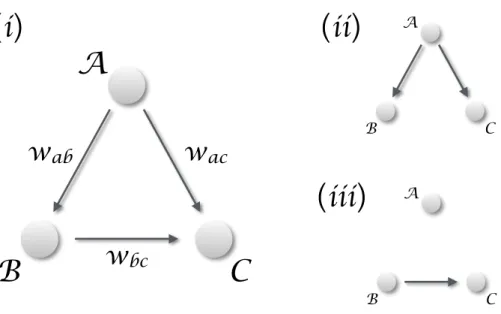
When only vectors of observations are available, i.e., vectors representing static observations of different realisations of the same system, it is customary to resort to statistics. This can be classical statistics, for then defining the relationship in terms of linear or non-linear correlations; or Bayesian statistics and the vast field of statistical learning and data mining (Vapnik,2013;Zanin et al.,2016). Although correlation, and statistical learning in general, appearprima facie as an interesting solution, they present the important drawback of not being able of discriminating between real and spurious causalities. Suppose one is studying a system composed of three interconnected elements, as the one depicted inFig. 1(i), with the aim of detecting if the dynamics of elementCis

causedbyB. Additionally, no time series are available, and elements are described through vectors of cross-sectional observations; in other words, multiple realisations of the same system are available, but each one of them can only be observed at a single moment in time. A statistically significant correlation betweenBandCmay be found both when a true causality is present (Fig. 1(iii)), and when both elements are driven by an unobserved confounding elementA(Fig. 1(ii)).

In order to tackle the scenario ofFig. 1, in this contribution we propose a novel metric for detecting causality from observational data. It entails three innovative points. First, it is defined on vectors of observation, which do not have to necessarily represent a time evolution. In other words, input vectors may correspond to gene expression levels measured in a population, i.e., to a cross-sectional study; or, but not necessarily, to multiple observations of the same subject, i.e., to a longitudinal study. Second, the method is based on the detection of extreme events, and on their appearance statistics. This is not dissimilar to Granger causality, as the latter measures how shocks in one time series are explained by a second one; but without the need of a time evolution. Third, it is optimised for the detection of non-linear causal relations, which are common in many real-world complex systems (Strogatz,2014), but that may create problems in standard causality metrics (Granger & Terasvirta,1993).

METHODS

A

B

C

w

w

w

A

B C

A

B C

(

i

₎

₍

ii

₎

(

iii

₎

Figure 1 Distinguishing causality from correlation.(i) General situation, in which three elementsA,B

andC_{interact in a simple triangular configuration. If one is interested in the relation between}B_andC_,

two different scenarios may arise. (ii) WhenAis dominating the dynamics, any common dynamics be-tweenB_andC_{will be a correlation, generated by the external confounding factor. (iii) The situation}

cor-responding to a real causality betweenBandC.

biomarkers in a same subject. In the case ofBandCbeing time series, clearly (bi,ci) would correspond to measurements at timei; yet, as already introduced, such dynamical approach is not required.

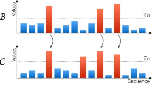
Starting from these vectors, some of their elements are labelled asextremewhen they exceed a threshold, i.e., bi> τb andci> τc. If a causality relation is present between them, such thatB→C, this should affect the way extreme events appear. First, under non-extreme dynamics, the two systemsB andC are loosely coupled. Especially when the relation is of a non-linear nature, small values in the former system are dampened during the transmission. Second, most of the extreme values ofBshould correspond to extreme values ofC, as extreme signals will be amplified from the former to the latter by the non-linear coupling. Third, extreme values ofConly partially correspond to extreme values ofB; due to its internal dynamics,C can display extreme events not triggered by the other element. An example of these three rules is depicted inFig. 2; note how extreme events (red bars) inBalways propagate toC, while the second extreme event ofCis caused by its internal dynamics and is not propagated.

Let us denote byp1the probability that an extreme event inCalso corresponds to an extreme event inB, i.e.,p1=P(bi> τb|ci> τc). Conversely,p2will denote the probability that an extreme event inBcorresponds to an extreme event inC, i.e.,p2=P(ci> τc|bi> τb). In the case of a real causality, the second condition implies thatp1≈1, the third one that

B

C

V

alues

V

alues

Sequence

!

!

Figure 2 Graphical representation of the proposed metric. A systemBis causing another systemC

when extreme values in the former, represented by red bars, propagate to the second; the opposite may nevertheless not happen, asC_{can also generate extreme values due to its own internal dynamics. The}

hor-izontal axis represents sequences of observations, but not necessarily a time evolution.

The previous analysis suggests that the necessary condition for having aB→Ccausality isp1>p2. The statistical significance can be quantified through a binomial two-proportion

z-test:

z=_q p1−p2

ˆp(1−ˆp)(_n1

1+

1 n2)

, (1)

withn1andn2the number of events associated top1andp2, andˆp=(n1p1+n2p2)/(n1+n2). The correspondingp-value can be obtained through a Gaussian cumulative distribution function.

Before demonstrating the effectiveness of the proposed causality metric, it is worth discussing several aspects of the same.

series comprising only a handful of values, it is still not applicable to static measurements, as for instance those found in genetics.

Second, the metric definition requires setting two thresholds, i.e.,τbandτc. This can be done usinga prioriinformation, e.g., when a level is accepted as abnormal for a given biomarker; or by simply explore all the parameters space, in order to assess the values of (τb,τc) corresponding to the lowestp-value. This may result especially useful in those situations for which the input elements are not well characterised: beyond the identification of causality relations, this method may also be used to define what an abnormal value is. Additionally, the form of detecting extreme events through a threshold is different from similar approached in the literature. For instance, Quiroga, Kreuz & Grassberger(2002) defines the events of interest as local maxima, independently of their amplitude; some of these events may not pass the threshold filtering here proposed, which only considers extreme (in the sense ofnot normalornot expected, but not necessarily ofmaximal) values.

Third, we have previously stated that the presence of a confounding effect can be correctly detected, and that in such situations the metric would not detect a statistically significant causality. According to the Common Cause Principle (Pearl, 2003), two variables are unconfoundediff they have no common ancestor in the causal diagram; and ensuring this requires including the confounding effects in the analysis, i.e., detect if there are causalities

A→BandA→Cin the diagram ofFig. 1. In the context here analysed, a confounding effect would be detected as the presence of co-occurring extreme events, generated by the confounding element, in both vectors of data. This requires the confounding element to influence in the same way both analysed elements, or, in other words, to have the same coupling strength between A→BandA→C. Additionally, if the causalityB→C

is mixed with an external influence, the latter cannot be detected if the strength of the former is greater—that is, a strong causality can mask a confounding effect. For all this, the proposed method does not always allow to discriminate true causalities from spurious relationships, although it provides important clues about which one of these two effects is having the strongest impact.

RESULTS

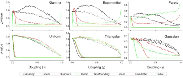
We first test the proposed metric with synthetic data.Figure 3presents the evolution of thep-value for two vectorsBandC, whose values are drawn from different distributions. Two situations are compared. First, a realB→Ccausality, such thatci=ci+γbn_i (nbeing the order of the coupling)—solid lines inFig. 3. Second, a confounding effect in which

bi=bi+γani andci=ci+γani—dashed lines inFig. 3. It can be appreciated that thep-values of real causalities drop to zero with small values of coupling constants; and that non-linear couplings perform better than linear ones. When the same analysis is performed using other causality standard metrics, such clear behaviour is not observed. Specifically, Fig. 4

0.0 0.2 0.4 0.6 p -v a lu e 0.0 0.2 0.4 0.6 Triangular Gaussian Uniform Pareto 0.0 0.2 0.4 0.6 0.8 Exponential Gamma

0.0 0.5 1.0 0.0 0.1 0.2 0.3 p -v a lu e

Coupling (γ)

Causality: Linear Quadratic Cubic Confounding: Linear Quadratic Cubic

0.0 0.5 1.0 0.0

0.1 0.2 0.3 0.4

Coupling (γ)

0.0 0.5 1.0 0.0

0.1 0.2 0.3 0.4

Coupling (γ)

Figure 3 p-value obtained by the proposed causality metric, for vectors of synthetic data drawn from

six different distributions, as a function of the coupling constantγ—see main text for details. Black, red and green lines respectively correspond to linear, quadratic and cubic couplings; solid lines depict true causalities (as inFig. 1(ii)), dashed lines spurious ones (Fig. 1(iii)). Each point corresponds to 10,000 real-isations.

Figure 4 p-value obtained by two standard causality metrics, for vectors of synthetic data drawn

from Gaussian distributions, as a function of the coupling constantγ. (A) Corresponds to the Granger Causality, (B) to the Transfer Entropy. Black, red and green lines respectively correspond to linear, quadratic and cubic couplings; solid lines depict true causalities (as inFig. 1(iii)), dashed lines spurious ones (Fig. 1(ii)).

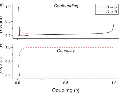
Figure 5 Evolution of thep-value of the causality, when considering bothB_→C_andC_→B_{tests for} a cubic coupling and for data drawn from a Gamma distribution (as in green lines of the first panel of

Fig. 3. (A) Reports the results for a confounding effect, (B) for a true causality betweenB_andC_.

causalities only requires calculating the two oppositep-values, and checking whether they are both small.

The necessity of detecting extreme events introduces a drawback in the method, i.e., the need of having a large set of input values to reach a stable statistics. This problem is explored inFig. 6, which depicts thep-value obtained as a function of the number of input values. Depending on the kind of relation to be detected, between 2 and 4 thousand values are required.

One of the advantages of the proposed metric is that it can be applied both to cross-sectional and longitudinal data. In other words, the metric can be used to study both those systems that do not present a temporal evolution, but for which information corresponding to different instances is available; and those systems whose evolution through time can be observed. Here we show such flexibility in the detection of the causality between two noisy Kuramoto oscillators (Kuramoto,2012;Rodrigues et al.,2016). Suppose two oscillators whose phases are defined as:

˙

φB=κB+ξ (2)

˙

φC=κC+γsin(φB−φC)+ξ . (3)

0 2 4 6 8 10 1E-5

1E-4 1E-3 0.01 0.1

p

-v

a

lu

e

Number of samples (thousands)

Linear Quadratic Cubic

Figure 6 Evolution of thep-value of the causality, for a triangular distribution, as a function of the number of values included in the input vectors. Black, red and green lines respectively correspond to lin-ear, quadratic and cubic couplings.

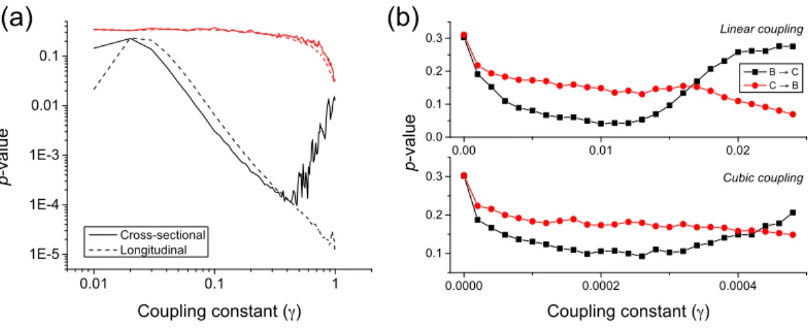
Figure 7 (A) Evolution of thep-value of the causality test between two Kuramoto oscillators, for different values of the coupling constantγ.Solid and dashed lines respectively correspond to a cross-sectional and longitudinal study—see main text for details. Black lines correspond to the proposed metric, red ones to Granger Causality. (B)p-value for two coupled Rössler oscillators as a function of the coupling constantγ, for a linear and cubic coupling.

Both the longitudinal and cross-sectional analyses yield similar results, suggesting that dynamical and static causalities are equivalent under the proposed metric. Only when the coupling is large, i.e., above 0.5, the longitudinal (i.e., time based) analysis yields betterp-values than the cross-sectional one, as the latter is probably confounded by the presence of a strong correlation.Figure 7Afurther depicts the behaviour of thep-value when calculated using the Granger Causality metric; it can be appreciated that the proposed causality metric is more sensitive, especially for small coupling constants.

An important characteristic of complex systems is that their constituting elements usually have a chaotic dynamics (Strogatz,2014), making more complicated the task of detecting causality between them. We here test the proposed metrics by considering two unidirectionally coupled Rössler oscillators (B→C) in their chaotic regime—see (Rulkov et al.(1995) for details. We consider both linear and cubic couplings; following the notation inRulkov et al.(1995), this means:

˙y1= −(y2+y3)−γ(y1−x1), and (4)

˙y1= −(y2+y3)−γ(y1−x1)3. (5)

Time series are created by sampling the second dimension of each oscillator (i.e.,x2and

y2) with a resolution lower than the intrinsic frequency.Figure 7Bdepicts the evolution of thep-value for low coupling strengthsγ, thus ensuring that the system isgeneralised synchronised. Forγ ≈0.01 (γ≈2·10−4_{for cubic coupling), a true causality is detected,} while forγ >0.015 (γ >4·10−4_{) the two oscillators start to synchronise.}

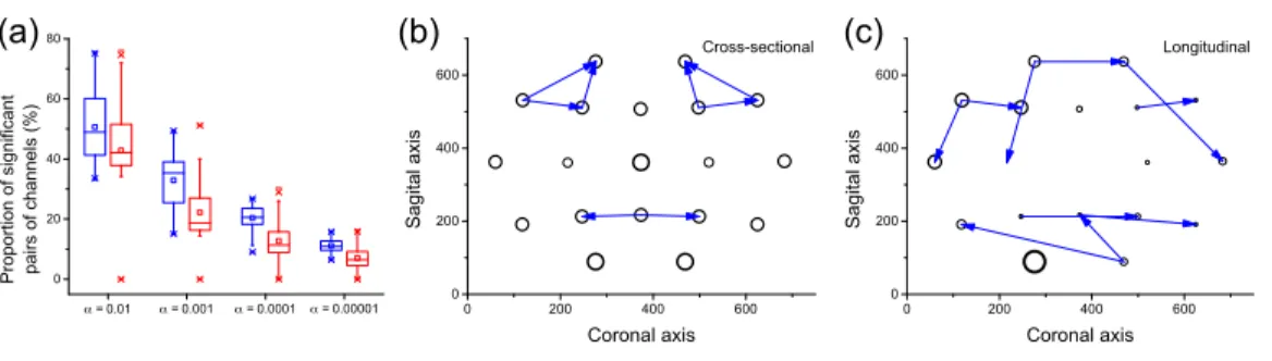
The possibility of combining a cross-sectional analysis of extreme values with a longitudinal analysis opens new doors towards the understanding of systems for which both aspects can be studied at the same time. Here we show how this can be achieved in the anal-ysis of functional networks representing the structure of brain activity in healthy subjects (Bullmore & Sporns,2009;Rubinov & Sporns,2010). The data set corresponds to electroen-cephalographic (EEG) recordings of 40 subjects during 50 trials of an object recognition task (details can be found inZhang et al.(1995) and references within), obtained through the UCI KDD archive (Bay et al.,2000). For each trial and subject, 19 time series of 256 samples were available, corresponding to one second of recording of 19 EEG channels in the 10–20 configuration. The longitudinal analysis was performed by calculating the causality using the raw time series. On the other hand, the cross-sectional analysis relies on identifying the propagation of extreme events, as in the case of the Kuramoto oscillators. Extreme events are defined as those for which the energy of the signal is maximum in a given time series; the energy is defined, at each time point, as the deviation with respect to the mean, normalised by the standard deviation of the signal—i.e., as the absolute value of the Z-Score.

Figure 8 Analysis of causality in EEG data. (A) Proportion of pairs of channels in which causality has been detected, for cross-sectional (blue) and longitudinal (red) analyses, as a function of the significance levelα. (B) Top-10 causality links in the cross-sectional analysis. (C) Top-10 causality links in the longitu-dinal analysis. In (B) and (C), the size of each node is proportional to its number of connections (i.e., its degree of participation in the cognitive task).

significant links, as detected by both analyses. While not completely equivalent, both graphs suggest that some areas are identified as active by both methods, e.g., the frontal lobe on the top and the visual and somatosensory integration area in the bottom. Remarkably, these two regions are expected to be relevant for the task studied, i.e., object identification: the former for higher function planning, i.e., react to the image shown, the latter in the processing of visual inputs.

CONCLUSIONS AND DISCUSSION

In conclusion, we presented a novel metric able to detect causality relationships both in static and time-evolving data sets, thus overcoming the limitation of existing metrics that rely on time series analysis. The proposed metric is designed to detect the propagation of extreme events, or shocks, and as such is more efficient when non-linear relations are present; it is further able to discriminate real from spurious causalities, thus enabling the detection of confounding effects. The effectiveness of the metric has been tested through synthetic data; data obtained from simple and chaotic dynamical systems, i.e., Kuramoto and Rössler oscillators; and through EEG data representing the activity of the human brain during an object recognition task.

In spite of the advantages that the proposed metric presents, and that have been described throughout the text, two limitations have to be highlighted. First, the reduced sensitivity of the metric to linear causality relationships, and in the analysis of data without long tail distributions, i.e., without clear extreme events—seeFig. 3for further details. Second, the need of large quantities of data, in the order of several thousands of observations, to reach statistically significant results (Fig. 6).

Nevertheless, data mining (and machine learning in general) is based on the Bayes theorem, a form of statistics of co-occurrences, and thus on a generalised concept of correlation. These methods are thus sensitive to the confounding effects that are frequently in place, as genes and metabolites create an intricate network of interactions. Resorting to classical causality metrics, like Granger’s one, is not possible, as time series are seldom available— measuring gene expression or metabolite levels is an expensive and slow process. In spite of this, causality is an essential element to be detected: if one only focuses on correlations, there is a risk of detecting elements whose manipulation does not guarantee the expected results on the system (Salmon et al.,2000;Cardon & Palmer,2003;Vakorin, Krakovska & McIntosh,2009). We foresee that the proposed causality metric can be an initial solution to this problem, by providing a causality test that can be applied to static data, and that could be used as the foundation of a new class of data mining algorithms.

A Python implementation of the proposed causality metric is freely available at

www.mzanin.com/Causality.

ADDITIONAL INFORMATION AND DECLARATIONS

Funding

The author received no funding for this work.

Competing Interests

Massimiliano Zanin is an Academic Editor for PeerJ and PeerJ Computer Science.

Author Contributions

• Massimiliano Zanin conceived and designed the experiments, performed the experiments, analyzed the data, wrote the paper, prepared figures and/or tables, reviewed drafts of the paper.

Data Availability

The following information was supplied regarding data availability: The data set used was downloaded from the UCI KDD archive at:

https://archive.ics.uci.edu/ml/datasets/EEG+Database.

Additionally, the source code for calculating the metrics can be downloaded from:

http://www.mzanin.com/Causality/.

REFERENCES

Bay SD, Kibler D, Pazzani MJ, Smyth P. 2000.The UCI KDD archive of large data sets for data mining research and experimentation.ACM SIGKDD Explorations Newsletter 2:81–85DOI 10.1145/380995.381030.

Bullmore E, Sporns O. 2009.Complex brain networks: graph theoretical analysis of structural and functional systems.Nature Reviews Neuroscience10:186–198

Cardon LR, Palmer LJ. 2003.Population stratification and spurious allelic association.

The Lancet 361:598–604DOI 10.1016/S0140-6736(03)12520-2.

Cios KJ, Moore GW. 2002.Uniqueness of medical data mining.Artificial Intelligence in Medicine26:1–24DOI 10.1016/S0933-3657(02)00049-0.

Donges JF, Schleussner C-F, Siegmund JF, Donner RV. 2015.Coincidence analysis for quantifying statistical interrelationships between event time series: on the role of flood events as possible drivers of epidemic outbreaks. ArXiv preprint.

arXiv:1508.03534.

Evans MG. 1959.Causality and explanation in the logic of Aristotle.Philosophy and Phenomenological Research19:466–485.

Gómez-Herrero G, Wu W, Rutanen K, Soriano MC, Pipa G, Vicente R. 2015.Assessing coupling dynamics from an ensemble of time series.Entropy 17:1958–1970

DOI 10.3390/e17041958.

Granger CWJ. 1988a.Causality, cointegration, and control.Journal of Economic Dynam-ics and Control12:551–559DOI 10.1016/0165-1889(88)90055-3.

Granger CWJ. 1988b.Some recent development in a concept of causality.Journal of Econometrics39:199–211.

Granger CWJ, Terasvirta T. 1993.Modelling non-linear economic relationships.OUP Catalogue.

Han J. 2002.How can data mining help bio-data analysis? In:Proceedings of the 2nd ACM SIGKDD workshop on data mining in bioinformatics (BIOKDD 2002), 1–2.

Hankinson RJ. 1998.Cause and explanation in ancient Greek thought. Oxford: Clarendon Press.

Hume D. 1965.An enquiry concerning human understanding. Alex Catalogue. Kuramoto Y. 2012.Chemical oscillations, waves, and turbulence.

Leslie AM, Keeble S. 1987.Do six-month-old infants perceive causality?Cognition

25:265–288DOI 10.1016/S0010-0277(87)80006-9.

Pearl J. 2003.Causality: models, reasoning, and inference.Econometric Theory

19:675–685.

Pearl J. 2009.Causality. Cambridge: Cambridge University Press.

Prather JC, Lobach DF, Goodwin LK, Hales JW, Hage ML, Hammond WE. 1997. Medical data mining: knowledge discovery in a clinical data warehouse. In: Proceed-ings of the AMIA annual fall symposium. Bethesda: American Medical Informatics Association, 101–105.

Quiroga RQ, Kreuz T, Grassberger P. 2002.Event synchronization: a simple and fast method to measure synchronicity and time delay patterns.Physical Review E66: 041904DOI 10.1103/PhysRevE.66.041904.

Rubinov M, Sporns O. 2010.Complex network measures of brain connectivity: uses and interpretations.Neuroimage52:1059–1069DOI 10.1016/j.neuroimage.2009.10.003. Rodrigues FA, Peron TJ, Ji P, Kurths J. 2016.The Kuramoto model in complex

Rulkov NF, Sushchik MM, Tsimring LS, Abarbanel HDI. 1995.Generalized syn-chronization of chaos in directionally coupled chaotic systems.Physical Review E

51:980–994DOI 10.1103/PhysRevE.51.980.

Salmon E, Collette F, Degueldre C, Lemaire C, Franck G. 2000.Voxel-based analysis of confounding effects of age and dementia severity on cerebral metabolism in Alzheimer’s disease.Human Brain Mapping10:39–48

DOI 10.1002/(SICI)1097-0193(200005)10:1<39::AID-HBM50>3.0.CO;2-B. Schreiber T. 2000.Measuring information transfer.Physical Review Letters85:461–464. Staniek M, Lehnertz K. 2008.Symbolic transfer entropy.Physical Review Letters100:

158101DOI 10.1103/PhysRevLett.100.158101.

Strogatz SH. 2014.Nonlinear dynamics and chaos: with applications to physics, biology, chemistry, and engineering. Boulder: Westview Press.

Tanaka SC, Balleine BW, O’Doherty JP. 2008.Calculating consequences: brain systems that encode the causal effects of actions.The Journal of Neuroscience 28:6750–6755

DOI 10.1523/JNEUROSCI.1808-08.2008.

Vakorin VA, Krakovska OA, McIntosh AR. 2009.Confounding effects of indirect connections on causality estimation.Journal of Neuroscience Methods184:152–160

DOI 10.1016/j.jneumeth.2009.07.014.

Vapnik V. 2013.The nature of statistical learning theory. Berlin, Heidelberg: Springer Science & Business Media.

Verdes PF. 2005.Assessing causality from multivariate time series.Physical Review E72: 026222DOI 10.1103/PhysRevE.72.026222.

Zanin M, Papo D, Sousa PA, Menasalvas E, Nicchi A, Kubik E, Boccaletti S. 2016. Combining complex networks and data mining: why and how.Physics Reports

635:1–44.

Zhang XL, Begleiter H, Porjesz B, Wang W, Litke A. 1995.Event related potentials during object recognition tasks.Brain Research Bulletin38:531–538