* Corresponding author.
E-mail address: [email protected] (K. Hassanlou) © 2017 Growing Science Ltd. All rights reserved. doi: 10.5267/j.dsl.2017.1.001
Decision Science Letters 6 (2017) 221–232
Contents lists available at GrowingScience
Decision Science Letters
homepage: www.GrowingScience.com/dsl
A multi period portfolio selection using chance constrained programming
Khadijeh Hassanloua*
a,School of Industrial Engineering, Khatam University, Tehran, Iran
C H R O N I C L E A B S T R A C T
Article history: Received October 3, 2016 Received in revised format: October 22, 2016
Accepted November 25, 2016 Available online
November 26 2016
This paper considers a portfolio selection problem with normally distributed returns and different rates for borrowing and lending. The primary concern is to determine the amount of investment in different planning horizons when the rate of borrowing is greater than the rate of lending. Chance constrained programming as an appropriate tool for addressing intrinsic uncertainty in portfolio selection problem is used. To solve this nonlinear programming, Genetic Algorithm is utilized. Numerical experiments are performed and the results are analyzed to present the performance of the proposed methodology.
Growing Science Ltd. All rights reserved. 7
© 201 Keywords:
Chance constrained programming Multi period portfolio selection Fuzzy programming
1. Introduction
Portfolio selection is defined as the selection of some assets to reach the investment’s goal. Markowitz (1952, 1956, 1959) is the first who offered Modern Portfolio Theory (MPT) where a quadratic objective function is minimized by considering some linear constraints. Markowitz’s MPT has been changed into paradigm in portfolio to construct a portfolio with the highest expected return at a given level of risk (the lowest level of risk at a given expected return).
programming approach to portfolio selection where the goals and constraints were fuzzy. They proposed a multi objective model taking into account three major criteria, i.e. return, risk and liquidity. Ammar and Khalifa (2003) introduced fuzzy portfolio optimization with a convex quadratic programming approach. Zhang and Nie (2004) proposed admissible efficient portfolio selection model under the assumption that the expected return and risk of asset have admissible errors to reflect the uncertainty in real investment actions. Tiryaki and Ahlatcioglu (2008) used fuzzy analytic hierarchy process (AHP) for portfolio selection. They revised fuzzy AHP addressing some of its fallacies, and called it revised constrained fuzzy AHP method. To reflect the uncertainty at the evaluation stage Chen and Huang (2009) represented rate of return and the variance as fuzzy numbers instead of the crisp representations used previously. Hung (2008) represented Mean-semi variance models for fuzzy portfolio selection using downside risk value and measures which only gauges the negative deviations from a reference return level, to replace variance.
In the second direction also we have some wealthy researches for example: initially Harlow and Rao (1989) proposed a framework for asset pricing based on generalized mean-lower partial moment. Simaan (1997) estimated risk value in portfolio selection as absolute deviation instead of variance and introduced a mean-absolute deviation model for portfolio selection problems. Williams (1997) utilized chance constraints concept in investment environment and maximized probability of achieving investment goals. Traditionally, as in above researches are, returns of individual securities were assumed to be stochastic variables (Yoshimoto, 1996; Best & Hlouskova, 2000).
When chance constrained programming (CCP) was introduced by Charnes and Cooper in 1959 as a tool to deal with uncertain decisions, it was believed that it could play important role in financial environment decisions. Charnes and Cooper (1959) defined chance constrained programming as: “select certain random variables as functions of random variables with known distributions in such a manner as (a) to maximize a functional of both classes of random variables subject to (b) constraints on these variables which must be maintained at prescribed levels of probability”.
Using chance constrained programming in financial decisions and portfolio analysis was initialed with Brockett et al. (1992), Charnes et al. (1993), Li (1995) and Williams (1997). Aouni et al. (2004) used chance constrained programming to model the portfolio selection problem by converting the stochastic compromise program into a deterministic one. Thereafter they developed their former chance constrained compromise programming model by considering conflicting in decision maker multi objectives previously seen in (Abdelaziz, 2005). Huang (2006) proposed two types of credibility-based portfolio selection model, according to two types of chance criteria: the objective was to maximize the investor’s return at a given threshold confidence level and the objective was to maximize the credibility of achieving a specified return level subject to the constraints.Yan (2009) represented security returns as bi-random variables and solved the portfolio selection problem according to bi-random theory. Asanga et al. (2014) developed a portfolio optimization problem under solvency constraints. They proposed a novel semiparametric formulation for each problem and explored a special class of multivariate GARCH models for modeling portfolio assets.
K. Hassanlou / Decision Science Letters 6 (2017)
The proposed model of this paper is a multi-period one because the single-period framework suffers from an important deficiency. It is normally hard to apply to long-term investors having different objectives at particular dates in the future, for which the investment decisions have to be accomplished in terms of temporal issues in addition to static risk-reward trade-offs. To satisfy this necessity, many researchers have developed this models towards formulating from the beginning the allocation problem over a horizon composed of multiple periods.
Bertsimas and Pachamanova (2008) applied robust optimization formulations for the multi period portfolio optimization problem. The multi-period portfolio optimization proposed by Bertsimas and Pachamanova (2008) could be developed to include realistic features such as borrowing and lending rates. The proposed method of this paper considers borrowing and lending rates as part of multi-period investment planning.
In this paper it is considered that the rates are stochastic variables with normal distributions and the results are discussed using a practical example. We believe this feature makes our proposed method more realistic since most of the brokerage houses provide the opportunity to make an acquisition on various assets by borrowing the money from the brokerage firms. This paper is organized as follows. First some preliminaries about chance constrained programming are presented in section2. In section 3 the proposed model is developed and described. The model is reformulated in chance constraint form in section 4.In Section 5 the characteristics of proposed GA is explained. Numerical results which research the performance of proposed model and also the GA are discussed in Section 6. Finally, in Section 7 conclusions are given to summarize the contribution of the paper.
2. Basic theorem in chance constraint programming
Chance Constrained Programming as the second type of stochastic programming, developed by Charnes and Cooper (1959), attempts to reconcile optimization over uncertain constraints. The constraints, which contain random variables, are guaranteed to be satisfied with a certain probability. In CCP, it is required that the objectives should be reached with the stochastic constraints held at least α of time, where α is provided as an appropriate safety margin by the decision maker.
Let x be a decision vector, ξbe a stochastic vector and gj(x, ξ) be stochastic constraint functions, j= 1,
2, …, p. Since the stochastic constraints gj(x, ξ) ≤ 0, j= 1, 2, …, p do not define a deterministic feasible
set, they need to be hold with a confidence level α. Thus chance constraint is represented as follows:
Pr { gj(x, ξ) ≤ 0, j= 1, 2, …, p } ≥α (1)
which is called a joint chance constraint, and when we want to consider them separately it is shown as follows:
Pr { gj(x, ξ) ≤ 0} ≥αj , j= 1, 2, …, p (2)
Theorem 1 (Liu, 2009) Assume that the stochastic vector ζ = (a1,a2,...,an,b)and the function g(x, ξ) has the form g(x, ξ) =a1x1a2x2 ...an xnb. If ai and b are assumed to be independently normally distributed random variables, then Pr { g(x, ξ) ≤ 0} ≥α if and only if
] [ ] [ ] [ )
( ]
[
1
2 1
1
b E b V x a Var x
a E
n
i
i i n
i
i
i
(3)
where Ф is the standardized normal distribution function.
3. The proposed model formulation
The following notations and parameters are used in the problem formulation,
N = the number of trading periods
m t
X = the investor’s dollar holdings in stock m at the beginning of period t, (which are fund with his capital);
(m= 0, 1... M) & (t=0, 1… N)
m t
X' = the investor’s dollar holdings in stock m at the beginning of period t, (which are fund with borrowing);
(m= 0, 1... M) & (t=0, 1… N)
m t
r = the return of stock m over time period (t, t + 1]; (m= 1, 2... M)
b t
r = the riskless borrowing rate over time period (t, t + 1]; (t=0, 1… N)
l t
r = the riskless lending rate over time period (t, t + 1]; (t=0, 1… N)
m t
u = the amount of stock m which is soled in period t; (m= 1... M) & (t= 1… N)
m t
v = the amount of stock m which is purchased in period t; (m= 1... M) & (t= 1… N)
m t
u' = the amount of m t
X' 1which is sold in period t; (m= 1... M) & (t= 1… N)
m t
v' = the amount of stock m which is purchased using credit in period t; (m= 1... M) & (t= 1… N)
V = the maximum permitted amount of buying for each stock in each period
WN = the investor’s final wealth at period N U(X) = the investor utility function
In this model, there are M risky assets and one riskless asset (asset 0) with unequal borrowing and lending rates i.e. b
t
r ≥ l
t
r . Now, one may invest using the existing cash or purchase more shares using
the credit with the borrowing rate. Let m t
X and m t
X' be the asset allocation held using the cash and the
credit, respectively. Therefore we have:
(P1) Max U= (
M m m N X 0 +
M m m N X 0' ) (4)
subject to
m t
X = (1+ m t
r 1) ( m t
X 1 − m t
u 1+ m t
v 1) , t = (1. . . N);m = (1. . . M), (5)
0
t
X = ( 1+ l t
r 1) ( 0 1
t
X +
M m m t u 1
1 −
M m m t v 1 1),t = (1. . . N), (6)
m t
X' = (1+ m t
r 1) ( m t
X' 1 − m t
u' 1+ m t
v' 1) t = (1. . . N); m = (1. . . M), (7)
0 't
X = ( 1− b t
r 1) ( 0 1 't
X +
M m m t u 1 1 ' −
M m m t v 1 1 ' ),t = (1. . . N), (8)
M m m t X 0≥β (
M m m t X 0
' ) t = (1. . . N), (9)
m t
v ≤ V; v'tm ≤ V t = (1. . . N); m = (1. . . M), (10)
K. Hassanlou / Decision Science Letters 6 (2017)
Note that any brokerage fund manager may ask his/her investors to have a balance between the margin and the cash allocated on different risky assets and this regulation is imposed on Eq. (9) where β determines the rate of balance.
As it can be seen in most of classical literature on portfolio optimization, the investor’s utility function is assumed to be concave to reflect aversion to risk but we consider a linear objective instead:
U (
M m m N X 0 +
M m m N X 0 ' ) ≈
M m m N X 0 +
M m m N X 0 ' (11)4. The proposed chance constrained strategy
As explained before in the proposed model of this paper for rendering the uncertainty and stochastic nature of portfolio selection problem it is assumed that the return rates ( m
t
r ) and borrowing and lending
rates ( b t
r and l t
r respectively), are independently and normally distributed random variables. So
stochastic constraints given in Eqs. (3-6) can be rewritten as follows:
Pr ( m t
X - (1+ m t
r 1) ( m t
X 1 − m t
u 1+ m t
v 1)) ≥α , t = (1. . . N); m = (1. . . M), (12)
Pr ( 0
t
X - ( 1+ l t
r 1) ( 0 1
t
X +
M m m t u 1
1 −
M m m t v 11)) ≥α ,
t = (1. . . N), (13)
Pr ( m t
X' - ( 1+ m t
r 1) ( m t
X' 1 − m t
u' 1+ m t
v' 1)) ≥α , t = (1. . . N); m = (1. . . M), (14)
Pr ( '0
t
X - ( 1− b t
r 1) ( 0 1 't
X +
M m m t u 1 1 ' −
M m m t v 1 1' )) ≥α , t = (1. . . N), (15)
As defined before, α is provided as an appropriate safety margin by the decision maker. Now according to Theorem 1, if m
t
r is normally distributed random variables N (E[rtm], Var[rmt ]) , b t
r is normally
distributed random variable N (E[rbt], Var[rbt]) and l t
r is normally distributed random variable N (E[
l t
r ], Var[rlt]), we can reformulate models as:
P2: max U =
M m m N X 0 +
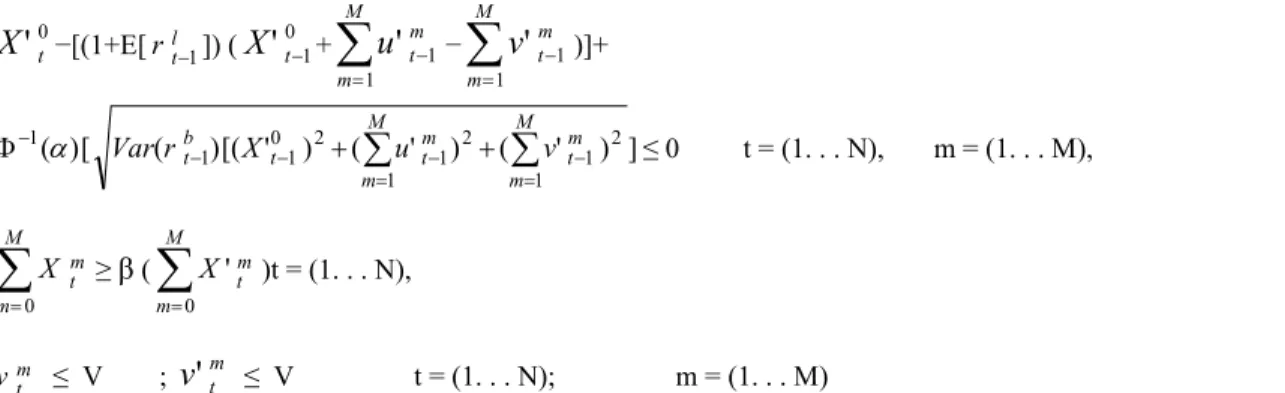
M m m N X 0 ' (16) subject to m tX − [(1+E[ m t
r 1]) ( m t
X 1− m t
u 1+vtm1)] + 1()[ Var(rtm1)[(Xtm1)2(utm1)2(vtm1)2]≤ 0 (17)
t= (1. . . N); m= (1. . . M),
0
t
X − [(1+E[ l t
r 1]) ( 0 1
t
X +
M m m t u 1
1−
M m m t v 1
1)] + ( )[ ( )[( ) ( ) ( ) ] 2 1 1 2 1 1 2 0 1 1
1
M m m t M m m t t l
t X u v
r Var
≤ 0
(18)
t = (1. . . N) ,m = (1. . . M)
m t
0 't
X −[(1+E[ l t
r 1]) (X't01+
M m m t u 1 1 ' −
M m m t v 1 1 ' )]+ ] ) ' ( ) ' ( ) ' [( ) ( [ ) ( 2 1 1 2 1 1 2 0 1 11
M m m t M m m t t b
t X u v
r Var
≤ 0 t = (1. . . N), m = (1. . . M),
(20)
M m m t X 0≥β (
M m m t X 0
' )t = (1. . . N),
(21)
m t
v ≤ V ; v'mt ≤ V t = (1. . . N); m = (1. . . M) (22)
To solve the proposed model, Genetic Algorithm is applied. The procedure of the proposed GA will be explained in Section 5.
5. Genetic algorithm
Complexity of many optimization problems is so high that conventional methods may not be able to solve them, successfully. Therefore evolutionary algorithms have been developed to solve such problems. Among them, Genetic Algorithm developed originally by Holland (1975), is one of the valid and popular heuristic techniques for solving optimization problems. GA is based on the mechanism of genetics and natural selection. Many studies have shown that GAs is capable of efficiently locating near optimal or even the optimal solutions for many combinatorial optimization problems.
The most common type of genetic algorithm works like this: a population is created with a group of individuals created randomly (chromosomes). The individuals in the population are then evaluated. The evaluation function or fitness function is originated by the objective function of the model and gives the individuals a score based on how well they perform at the given task. Two individuals are then selected based on their fitness, the higher the fitness, the higher chance of selection. These individuals then “reproduce” to create one or more offspring, after which the offspring are mutated randomly. This continues until a suitable solution has been found or a certain numbers of generations have passed, depending on the needs of the programmer. In Fig. 1, the pseudo-code for typical Evolutionary Algorithm is represented.
Fig. 1. Pseudo-code for typical EA
The proposed GA of this paper has been coded in MATLAB 7.6 based on the following issues,
BEGIN
INITIALIZE population with random candidate solutions;
EVALUATE each candidate;
REPEAT UNTIL (TERMINATION CONDITION
is satisfied) DO 1. SELECT parents;
2. RECOMBINE pairs of parents; 3. MUTATE the resulting offspring; 4. EVALUATE new candidate; 5. SELECT individuals for the next
K. Hassanlou / Decision Science Letters 6 (2017)
a) Fitness function: which is introduced before, in this paper is defined as the objective function
of model P2 i.e.
U=
M
m m N
X 0
+
M
m m N
X 0
' is selected as the fitness function.
b) Structure of genes and chromosomes: as discussed before, each chromosome represented the potential and feasible solution. For the proposed model of this paper (P2), each chromosome consists of 6 fundamental parts as: X,Xp,u,up,v,vp. Length of chromosome indicates the number of variables in problem and in this case the number of variables can be obtained from 2×(M+1)×(N+1)+4×M×N.
c) Operators: three main operators should be defined for GA as follow:
Selection operator: The selection function, stochastic uniform, lays out a line in which each parent corresponds to a section of the line of length proportional to its scaled value. The algorithm moves along the line in steps of equal size. At each step, the algorithm allocates a parent from the section it lands on. The first step is a uniform random number less than the step size.
Crossover function: In proposed GA, Scattered crossover function is used, where this type of crossover creates a random binary vector where the length of binary vector is equal to the parent’s vector length. So, the genes are selected from the first parent where the vector’s element is a 1, and from the second one where the vector is a 0, and combines the genes to form the first child, and verse versa to form the second one. Meanwhile, dynamically, all of the constraints monitor the characteristics of generated childe and if it is not feasible, the process of cross over will be repeated.
Mutation function: mutation options specify how the genetic algorithm makes small random changes in the individuals in the population to create mutation children. Mutation provides genetic diversity and enables the genetic algorithm to search a broader space. For the proposed GA, Gaussian mutation is selected. Gaussian, adds a random number taken from a Gaussian distribution with mean 0 to each entry of the parent vector. The standard deviation of this distribution is determined by the parameters Scale and Shrink, which are displayed when we select Gaussian, and by the Initial range setting in the Population options. The Scale parameter determines the standard deviation at the first generation. The Shrink parameter controls how the standard deviation shrinks as generations go by.
In section 6numerical results of an example are analyzed and the proposed GA will be verified.
6. Numerical results
This section is organized in three parts: first the parameters of proposed GA are set, second a numerical example is implemented with proposed GA and the results are analyzed, third to validatethe proposed GA (which is coded by MATLAB 7.6), we compared the results with the results of the implementation of the fuzzy model, which were available in the literature.
6.1. Parameter setting
“PopulationSize” indicates the size of population that arises from the number of variables in problem. In this proposed GA, as it mentioned before, number of variables can be obtained from 2×(M+1)×(N+1)+4×M×N.
“TolCon” is used to determine the feasibility with respect to nonlinear constraints and better value for it in this case is 10 -24. Finally, “TolFun” specifies that the algorithm runs until the cumulative change in the fitness function value is less than TolFun, so to avoid from halting the algorithm in initial iterations we get it small value as 10 -30.
6.2. Running a numerical example
In this section an example is considered to illustrate the results of the proposed model using GA. Let us consider M= 10 (one risk free asset and nine risky assets) and N= 4 (t= 0 …4). For the risky assets, we picked nine stocks which have more weight in the Dow Jones Index based on last published factsheet in 2010: IBM, MMM, CVX, CAT, MCD, UTX, BA, XOM and JNJ representing of over 50% of the Dow Jones Index. The daily closing prices from 2010to the end of 2014, are used to estimate their means and variances.
The return of the risk-free asset (lending rate) obtained from the information of daily 13-week US treasury bills data from 2010to 2014. Borrowing rate data is obtained from US annual prime rates. The Prime Interest Rate is the interest rate charged by banks to their most creditworthy customers (usually the most prominent and stable business customers).
Security return rates, borrowing and lending rates are normally distributed random variables presented as follow. Table 1 shows the expected rate of returns for risky assets and borrowing and lending rates in planning time periods (i.e. E[rmt ],E[rlt], E[rbt] in P2).
Table 1
Expected value of risky assets return, lending and borrowing rates
t = 1 t = 2 t = 3 t = 4
IBM 8.84% 2.92% -2.64% 3.56%
MMM 11.93% 0.71% 2.97% -9.18%
CVX 11.21% 1.44% 5.66% -6.73%
CAT 17.17% 0.68% -2.82% -2.80%
MCD 7.52% 3.16% 9.51% -2.36%
UTX 9.08% 1.09% -0.35% -0.64%
BA 14.84% -6.3% -3.41% -2.65%
XOM 3.87% 0.28% 8.50% -6.33%
JNJ 4.42% 3.64% 1.10% -5.58%
Bill rates 0.56% 0.57% 0.47% 0.60%
Prime rates 1.39% 1.40% 1.36% 1.46%
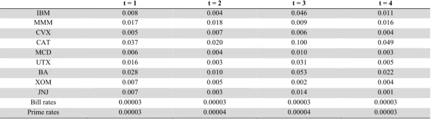
Table 2 shows the variance of historical return rates for risky assets, lending and borrowing (i.e. Var (
m t
r ),Var (rlt),Var (rbt) in P2).
Table 2
Variance of historical return for risky assets, lending and borrowing rates
t = 1 t = 2 t = 3 t = 4
IBM 0.008 0.004 0.046 0.011
MMM 0.017 0.018 0.009 0.016
CVX 0.005 0.007 0.006 0.004
CAT 0.037 0.020 0.100 0.049
MCD 0.006 0.004 0.010 0.003
UTX 0.016 0.003 0.031 0.005
BA 0.028 0.010 0.053 0.022
XOM 0.007 0.005 0.002 0.004
JNJ 0.007 0.003 0.014 0.001
Bill rates 0.00003 0.00003 0.00003 0.00003
K. Hassanlou / Decision Science Letters 6 (2017)
The proposed chance constrained model has been solved using this data with β=1 and moreover the initial values for investor’s holdings in first period (t=0) need to be considered.
Table 3 demonstrates the results of implementation of the proposed GA for developed model and a given example.
Table 3
The results of the implementation of GA for the proposed model
Time period t = 0 t = 1 t = 2 t = 3 t = 4
In
ve
st
or
hol
dings
in
e
ach period
0
t
X 1000 391.4 581.34 391.9 72758
1
t
X 10,000 2609.3 3266 1959.6 126.6
2
t
X 9000 2609.3 2612.8 2612.8 62.2
3
t
X 8000 4566.4 3200.6 3914.1 52.4
4
t
X 7000 3261.7 3266 5813.4 187.1
5
t
X 6000 1304.7 2612.8 3914.1 237.1
6
t
X 5000 5153.5 3919.2 1959.6 652.4
7
t
X 4000 5153.5 653.2 1306.4 250.1
8
t
X 3000 2609.3 1306.4 2612.8 61.7
9
t
X 2000 2609.3 1306.4 1306.4 160.9
0
't
X 1000 319.6 254.4 260.9 68382
1
't
X 10,000 3914.1 1957 3848.8 231
2
't
X 9000 2609.3 1891.8 4566.4 98.9
3
't
X 8000 3196.5 1957 2609 72.2
4
't
X 7000 1304.7 3261.7 1957 120
5
't
X 6000 1957 2609.4 1957 230.5
6
't
X 5000 71758 3196.5 1957 645.8
7
't
X 4000 3261.7 2609.4 4501.2 176.2
8
't
X 3000 7175.8 6523.5 3261.7 158.8
9
't
X 2000 1957 2609 3914 206.1
U 143,743.2
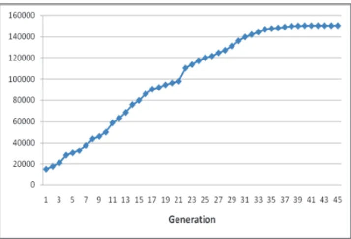
Fig. 2.Improvement of objective function over generations
6.2. Comparing GA and LINGO
In order to verify the proposed methodology, an example used in the previous section is considered and the results of the proposed GA for stochastic model (which is coded by MATLAB 7.6) are compared with the results of implementation of LINGO software package. Because of LINGO’s limitations to reach the optimal solutions in nonlinear problems, the linear multi period portfolio selection introduced by Sadjadi et al. (2011) is considered for validation.
In linear fuzzy model, the return rates and also borrowing and lending rates are represented as triangular fuzzy numbers because these rates are not exactly known for the future planning. The proposed fuzzy model has been implemented with confidence level as 1in LINGO. For comparing the results we have considered different values for β for the proposed models and implemented them with both LINGO and GA. Objective function values for different values of β are shown in Table 4.
Table 4
The results of the proposed model versus optimal solutions obtained Lingo software package
β Objective function (U)
LINGO GA
0 [140173.1, 149860.5] 151768.8
0.2 [139552.4, 148079.1] 150075
0.5 [137671.9, 146412] 147556.1
0.8 [135413.7, 144713.5] 147012.9
1 [134879.4 , 143516.2] 144870
As it can be understood, from Table 4, the results of chance constrained model with proposed GA is clearly better than the results of Fuzzy model solved by LINGO. The results show us differences between LINGO’s global optimum (maximum U with α = 0) and GA’s best objective values, i.e. we can improve the investor utility be developing chance constrained portfolio selection model using the proposed model. As mentioned before, in this paper the borrowing and the lending rates are considered to be different, i.e. borrowing and short selling with different interest rates are permitted.
7. Conclusions
K. Hassanlou / Decision Science Letters 6 (2017)
independently and normally distributed random variables. A Genetic Algorithm coded by MATLAB 7.6 software has been generated to solve the proposed model which belongs to nonlinear programming (NLP).To validate the proposed model the results of some real-life numerical example has been compared with the results of Fuzzy model solved by LINGO. This comparison shows us that we could improve investor’s utility by developing new chance constrained model and solving it by proposed GA.
References
Abdelaziz, F. B., Aouni, B., & El Fayedh, R. (2007). Multi-objective stochastic programming for
portfolio selection. European Journal of Operational Research, 177(3), 1811-1823.
Ammar, E., & Khalifa, H. A. (2003). Fuzzy portfolio optimization a quadratic programming
approach. Chaos, Solitons & Fractals, 18(5), 1045-1054.
Aouni, B., Abdelaziz, F. B., & El-Fayedh, R. (2000). Chance constrained compromise programming
for portfolio selection. Laboratoire LARODEC, Institut Superieur de Gestion, La Bardo.
Asanga, S., Asimit, A., Badescu, A., & Haberman, S. (2014). Portfolio optimization under solvency
constraints: a dynamical approach. North American Actuarial Journal, 18(3), 394-416.
Bertsimas, D., & Pachamanova, D. (2008). Robust multiperiod portfolio management in the presence
of transaction costs. Computers & Operations Research, 35(1), 3-17.
Best, M. J., & Hlouskova, J. (2000). The efficient frontier for bounded assets. Mathematical Methods
of Operations Rresearch, 52(2), 195-212.
Brockett, P. L., Charnes, A., Cooper, W. W., Kwon, K. H., & Ruefli, T. W. (1992). Chance constrained
programming approach to empirical analyses of mutual fund investment strategies. Decision
Sciences, 23(2), 385-408.
Charnes, A., & Cooper, W. W. (1959). Chance-constrained programming. Management Science, 6(1),
73-79.
Charnes, A., Cooper, W.W., Kwon, K.H., & Ruefli, T.W. (1993). Chance constrained programming and other approaches to risk in strategic management. In: L. Gould, P. Halpern (Eds.).Proceedings of a Conference in Honor of M.J. Gordon, Social Science Research Council of Canada, Ottawa.
Chen, L. H., & Huang, L. (2009). Portfolio optimization of equity mutual funds with fuzzy return rates
and risks. Expert Systems with Applications, 36(2), 3720-3727.
Gupta, P., Inuiguchi, M., Mehlawat, M. K., & Mittal, G. (2013). Multiobjective credibilistic portfolio
selection model with fuzzy chance-constraints. Information Sciences, 229, 1-17.
Harlow, W. V., & Rao, R. K. (1989). Asset pricing in a generalized mean-lower partial moment
framework: Theory and evidence. Journal of Financial and Quantitative Analysis, 24(03), 285-311.
Holland, J. H.(1975). Adaptation in natural and artificial systems: An introductory analysis with applications to biology, control and artificial intelligence.University of Michigan Press.
Huang, X. (2006). Fuzzy chance-constrained portfolio selection. Applied Mathematics and
Computation, 177(2), 500-507.
Huang, X. (2008). Mean-semivariance models for fuzzy portfolio selection. Journal of Computational
and Applied Mathematics, 217(1), 1-8.
Li, S. X. (1995). An insurance and investment portfolio model using chance constrained
programming. Omega, 23(5), 577-585.
Liu, B.(2009).Theory and Practice of Uncertain Programming. 3rd ed. UTLAB.
Markowitz, H. (1952). Portfolio selection. The Journal of Finance, 7(1), 77-91.
Markowitz, H. (1956). The optimization of a quadratic function subject to linear constraints. Naval
Research Logistics Quarterly, 3(1‐2), 111-133.
Markowitz, H.(1959).Portfolio selection: Efficient diversification of investments. New York: Wiley.
Parra, M. A., Terol, A. B., & Urıa, M. R. (2001). A fuzzy goal programming approach to portfolio
selection. European Journal of Operational Research, 133(2), 287-297.
Qin, Z., Wang, D. Z., & Li, X. (2013). Mean-semivariance models for portfolio optimization problem
with mixed uncertainty of fuzziness and randomness. International Journal of Uncertainty,
Qin, Z. (2015). Mean-variance model for portfolio optimization problem in the simultaneous presence
of random and uncertain returns. European Journal of Operational Research, 245(2), 480-488.
Sadjadi, S. J., Seyedhosseini, S. M., & Hassanlou, K. (2011). Fuzzy multi period portfolio selection
with different rates for borrowing and lending. Applied Soft Computing, 11(4), 3821-3826.
Simaan, Y. (1997). Estimation risk in portfolio selection: the mean variance model versus the mean
absolute deviation model. Management Science, 43(10), 1437-1446.
Sun, Y., Aw, G., Loxton, R., & Teo, K. L. (2017). Chance-constrained optimization for pension fund
portfolios in the presence of default risk. European Journal of Operational Research, 256(1),
205-214.
Tiryaki, F., & Ahlatcioglu, B. (2009). Fuzzy portfolio selection using fuzzy analytic hierarchy
process. Information Sciences, 179(1), 53-69.
Williams, J. O. (1997). Maximizing the probability of achieving investment goals. The Journal of
Portfolio Management, 24(1), 77-81.
Yan, L. (2009). Chance-constrained portfolio selection with birandom returns. Modern Applied
Science, 3(4), 161.
Yoshimoto, A. (1996). The mean-variance approach to portfolio optimization subject to transaction
costs. Journal of the Operations Research Society of Japan, 39(1), 99-117.
Zhang, W. G., & Nie, Z. K. (2004). On admissible efficient portfolio selection problem. Applied
Mathematics and Computation, 159(2), 357-371.