www.hydrol-earth-syst-sci.net/20/4717/2016/ doi:10.5194/hess-20-4717-2016
© Author(s) 2016. CC Attribution 3.0 License.
Delineation of homogenous regions using hydrological variables
predicted by projection pursuit regression
Martin Durocher1, Fateh Chebana2, and Taha B. M. J. Ouarda2,3
1Université du Québec à Trois-Rivières, University of Québec, 3351, Blvd. des Forges, C.P. 500, Trois-Rivières,
G9A 5H7, Canada
2Institut National de Recherche Scientifique (INRS-ETE), University of Québec, 490 de la Couronne, Québec,
G1K 9A9, Canada
3Institute Center for Water Advanced Technology and Environmental Research (iWater), Masdar Institue of Science and
Technology, P.O. Box 54224, Abu Dhabi, UAE
Correspondence to:Martin Durocher ([email protected])
Received: 11 March 2016 – Published in Hydrol. Earth Syst. Sci. Discuss.: 31 March 2016 Revised: 12 October 2016 – Accepted: 29 October 2016 – Published: 29 November 2016
Abstract.This study investigates the utilization of hydrolog-ical information in regional flood frequency analysis (RFFA) to enforce desired properties for a group of gauged stations. Neighbourhoods are particular types of regions that are cen-tred on target locations. A challenge for using neighbour-hoods in RFFA is that hydrological information is not avail-able at target locations and cannot be completely replaced by the available physiographical information. Instead of us-ing the available physiographic characteristics to define the centre of a target location, this study proposes to introduce estimates of reference hydrological variables to ensure a bet-ter homogeneity. These reference variables represent nonlin-ear relations with the site characteristics obtained by projec-tion pursuit regression, a nonparametric regression method. The resulting neighbourhoods are investigated in combina-tion with commonly used regional models: the index-flood model and regression-based models. The complete approach is illustrated in a real-world case study with gauged sites from the southern part of the province of Québec, Canada, and is compared with the traditional approaches such as re-gion of influence and canonical correlation analysis. The evaluation focuses on the neighbourhood properties as well as prediction performances, with special attention devoted to problematic stations. Results show clear improvements in neighbourhood definitions and quantile estimates.
1 Introduction
Accurate estimates of the risk of occurrence of extreme hy-drological events are necessary for the minimization of the impacts of these events and for the optimal design and man-agement of water resource systems. However, necessary in-formation is not always available at the sites of interest. It is hence necessary to develop procedures to transfer, or to regionalize, the available information at existing gauged sites to the ungauged ones. regional flood frequency analy-sis (RFFA) represents a large class of techniques commonly used in water sciences to evaluate the risk of occurrence of extreme hydrological phenomena of rare magnitudes at ungauged locations (Haddad and Rahman, 2012; Hosking and Wallis, 1997; Laio et al., 2011; Pandey, 1998; Reis et al., 2005).
unob-served hydrological behaviour from available hydrological and physio-meteorological information.
Neighbourhoods are specific forms of regions that are not composed of a fixed set of stations, but are rather composed of gauged sites that are the most similar to a given target site. Hence, two distinct target locations will have their own dis-tinct neighbourhoods which may overlap. Comparative stud-ies have shown that neighbourhoods will lead to better re-gional estimates than fixed regions (Burn, 1990; Ouarda et al., 2008; Tasker et al., 1996). To identify the most similar gauged sites in terms of hydrological properties, a notion of distance is needed. It allows to evaluate the proximity, or rel-evance, of each gauged site to the target location and to iden-tify the most hydrologically similar gauged sites. However, when the target location is ungauged, this distance cannot be directly calculated due to the missing hydrological infor-mation. Physio-meteorological information is hence used for similarity evaluation. The traditional approach, based on the distance between site characteristics, is commonly referred to as the region of influence (ROI) model (Burn, 1990), which received particular attention in the hydrological literature. The focus was mainly on the estimation of the model pa-rameters where, for instance, generalized least squares were used to account for unequal variability in the at-site estima-tions (e.g. Griffis and Stedinger, 2007; Stedinger and Tasker, 1985) and to deal with the presence of spatial correlation (e.g. Kjeldsen and Jones, 2009).
Alternatively, Ouarda et al. (2001) used canonical correla-tion analysis (CCA) to build neighbourhoods from a canoni-cal distance that accounts for the interrelation between flood quantiles and site characteristics. For this method, neighbour-hoods are formed by gauged sites that are the most similar to the target location, according to the distance between vectors of flood quantiles corresponding to different return periods. The CCA method in RFFA estimates the unavailable hydro-logical variables as linear combinations of site characteris-tics. Consequently, the available site characteristics are trans-formed into more meaningful hydrological quantities for the purpose of delineating neighbourhoods. However, the CCA method suffers from some limitations, such as linearity and normality assumptions (He et al., 2011). Subsequent studies have aimed at improving the CCA method by improving the CCA technique itself (Chebana and Ouarda, 2008; Ouali et al., 2015). However, little attention has been paid to the im-portance of properly choosing the hydrological quantities in the delineation step, whereas much effort has been devoted to the modelling step. Indeed, Chebana and Ouarda (2008) em-ployed an iterative linear procedure to estimate neighbour-hood centres and they showed that the quality of these cen-tres’ estimates is the crucial element to the improvement of the final model performance.
The present study aims to provide a general framework with more flexibility regarding the linearity and normality assumptions. This is achieved by replacing CCA in the prior analysis of hydrological variables by projection pursuit
re-gression (PPR), a nonparametric rere-gression method recently considered as an estimation model in RFFA (Durocher et al., 2015). The present study is also interested in assessing the advantages of employing hydrological variables other than the at-site flood quantiles in prior modelling as well as considering a combination of these hydrological variables with site characteristics.
L-moments have already been used in RFFA to test the homogeneity of fixed regions when the target site is gauged (Chebana and Ouarda, 2007; Hosking and Wallis, 1997). In the present study, the prediction of the L-moments at un-gauged sites is also considered to improve the delineation of the neighbourhoods by reducing uncertainties. Moreover, a conceptual advantage of using L-moments conversely to at-site flood quantiles is that the L-moments do not depend on the subjective selection of at-site distributions.
The present paper is organized as follows. Section 2 presents the background material for the techniques used in the present research. Section 3 elaborates on the prior anal-ysis of hydrological variables and their integration with the techniques presented in Sect. 2 to form a complete proce-dure. Section 3 also suggests criteria for the evaluation of the predictive performances and the neighbourhood properties. Section 4 illustrates the application of the method in a case study. Traditional ROI and CCA methods serve as references in order to evaluate the relative performance of the investi-gated method. Finally, concluding remarks are provided in Sect. 6.
2 Background
2.1 Delineation of neighbourhoods
In RFFA, neighbourhoods are used to identify gauged sites from which information is transferred to the target loca-tion. A neighbourhood is characterized by a centre and a radius that delimits an area (not necessary in the geograph-ical sense). Gauged sites inside the area delineate a region that includes relevant sites to the target location. At each site
i=1, . . ., n,p characteristicsxi= xi,1, . . ., xi,pare
avail-able. Typically, the ROI method forms neighbourhoods ac-cording to a radius based on a metricd:
d xi,xj=
v u u t
p X
k=1
(xi,k−xj,k)2
σk2 , (1)
whereσk is the standard deviation ofxi,k n
i=1, thekth site
characteristic (Eng et al., 2005).
Alternatively, CCA is a multivariate technique used to un-veil the interrelation between two groups of variables. Let
linear combinations of the original random variables:
Uk=akX, (2)
Vk=bkY, (3)
where the correlations ρk=corr(Uk, Vk) are
sequen-tially maximal for k=1, . . ., K under the conditions corr(Uk, Ul)=corr(Vk, Vl)=0 for k6=l. Only the
canon-ical pairs(Uk, Vk)with unit variances are considered.
To delineate neighbourhoods, the CCA approach con-siders the canonical scores ui=(a1, . . ., ar)′xi and vi=
(b1, . . ., br)′yi that are, respectively, linear combinations of
site characteristics xi and flood quantiles corresponding to
different return periods yi for site i. Due to the missing hydrological information at the ungauged location denoted
i=0, the flood quantiles y0 and the corresponding linear combinationv0are unknown. Nevertheless, CCA provides a
linear estimatev0≈3u0, where3=diag(ρ1, . . ., ρK).
Ac-cordingly, a neighbourhood is delineated in the canonical space based on the distance:
d(vi, 3u0)=(vi−3u0)′
I−32−
1
(vi−3u0) . (4)
More details on the CCA approach in RFFA can be obtained in Ouarda et al. (2001) and Ouarda (2016).
2.2 Multiple regression
In RFFA, two types of regional models are often considered to predict flood quantiles corresponding to given return pe-riods: the index-flood model and the regression-based model (Ouarda et al., 2008). The index-flood model predicts a tar-get distribution by assuming that all distributions inside the region are proportional to a regional distribution, up to a scale factor called index flood. The flood quantile of interest at a target location is then calculated from the regional distribu-tion based on the predicted index flood (e.g. Chebana and Ouarda, 2009; Dalrymple, 1960; Stedinger and Lu, 1995). Conversely, the regression-based model considers directly the at-site estimates of the desired flood quantiles for predic-tion. Flood quantiles are then predicted at their target loca-tions by the regression equaloca-tions estimated within the neigh-bourhoods (Pandey and Nguyen, 1999).
Even though they proceed differently, both the index-flood model and the regression-based model may use the same multiple regression techniques to transfer information to an ungauged location. For the sake of simplicity, the term hydro-logical variables is used to designate the corresponding out-put variableszi of these models at locationi=1, . . ., n.
Con-sequently, for the index-flood model, zi is the index flood,
while for a regression-based model the hydrological variable
zi is the flood quantile corresponding to the return period of
interest.
Multiple regression models assume linear interrelation be-tween the hydrological variableziand the site characteristics
xi. Consequently, in several cases, transformations are
nec-essary to meet this assumption. For instance, the power law form is frequently used to model flood quantiles:
zi =eβ0×xi,β11×. . .×x βp
i,p×εi, (5)
whereβ′= β0, β1, . . ., βpare parameters andεi is an error
term. Applying a logarithmic transformation is sufficient to cast Eq. (5) into a linear model. In general, a proper transfor-mation is assumed for the hydrological variablesyi=g (zi)
being linearly related to the site characteristics.
In line with previous notations, lety=(y1, . . ., yn)be the
hydrological variables, X be the design matrix of the site characteristicsxi,j with intercept andε=(ε1, . . ., εn)be the
error term. Hence, in matrix notation, a multiple regression model has the form
y=Xβ+ε, (6)
and according to the least-squares theory, the estimates of the parameters are
ˆ
β= X′X−1
X′y. (7)
2.3 Projection pursuit regression
Some methods predict hydrological variables without the formation of regions, such as physiographical kriging (Cas-tiglioni et al., 2009; Chokmani and Ouarda, 2004), general-ized additive models (Chebana et al., 2014) and artificial neu-ral networks (Dawson et al., 2006; Ouarda and Shu, 2009). More recently, PPR was introduced to provide a flexible non-parametric regression approach to describe the nonlinearity that is present in the relationship between hydrological vari-ables and site characteristics. PPR was used in the RFFA con-text by Durocher et al. (2015) to directly predict flood quan-tiles without delineation.
The basic elements of a PPR model arek=1, . . ., m func-tionsfk called terms and defined as
fk(X)=gk α′kX
, (8)
where directionsαk are vectors of coefficients and gk are
smooth functions. The directionsαk are coefficients that
re-spect|α| =1 and determine a predictorαk′Xas relevant linear combinations of the site characteristicsX. The terms are then combined into a regression model:
y=µ+
m X
k=1
fk(X)+ε, (9)
whereµ is the global mean andε is an error term. Notice that the orthogonality between directionsαkis not imposed;
The componentsαkandgkof the model in Eq. (9) are
esti-mated by the least-squares approach (Friedman et al., 1983). For a unique direction (m=1), PPR can be estimated by standard nonlinear algorithms (Yu and Ruppert, 2002) but, in general, a stage-wise algorithm is adopted to find a proper solution (Friedman and Tukey, 1974). Comparative studies show that PPR has a predictive performance that is similar to artificial neural networks (Bishop, 1995; Hwang et al., 1994). However, Durocher et al. (2015) indicated that in RFFA, PPR reduces to more parsimonious models than artificial neural networks, which provides an explicit expression of the re-gression equations.
3 Methodology
The present study deals with neighbourhood delineation and focuses more precisely on the identification of reliable es-timates of the hydrological centres of these neighbourhoods. For the sake of simplicity, the variables forming these centres will be referred to as reference variables, because they rep-resent the reference used to evaluate the similarity between a target location and the gauged sites. Reference variables can take different forms, such as site characteristics, hydrological variables or a combination of both. Their nature is important, because it determines the properties that are deemed to be im-portant between close sites. The particularity of the present method is that PPR can be used to predict these neighbour-hood centres (prior to the RFFA modelling step) when some of the reference variables are unknown hydrological vari-ables. Accordingly, the proposed method will be referred to as RVNs for reference variable neighbourhoods.
3.1 Estimation of the reference variables
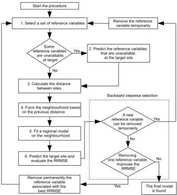
The general procedure can be described by the steps below: 1. Select the reference variables.
2. If necessary, predict the reference variables that are not available at the target site.
3. Compute the distance between sites.
4. Form the neighbourhood based on the previous dis-tance.
5. Fit a regional model on the neighbourhood.
6. Predict the target site and evaluate a performance crite-rion.
In step 1, the selection of a set of the reference variables can be subjective and depends on the problem at hand. In the present study, the backward step-wise selection procedure is considered to remove, from an initial set of reference vari-ables, those that do not contribute to the prediction power of the model. This selection procedure is more objective and
2. Predict the reference variables that are unavailable
at the target site
3. Calculate the distance between sites
4. Form the neighbourhood based on the previous distance
Some reference variables
are unavailable at target
1. Select a set of reference variables
6. Predict the target site and evaluate the RRMSE 5. Fit a regional model
on the neighbourhood
A new reference variable
can be removed temporarily
Yes
Remove permanently the reference variable associated with the best RRMSE
Removing one reference variable
improves the RRMSE Yes
No
No
The final model is found Yes
No Start the procedure
Backward stepwise selection Remove the reference
variable temporarily
Figure 1.Diagram of the RVN method using backward step-wise selection.
depends on a performance criterion. In the present study, the relative root mean square error (RRMSE) criterion is cho-sen for this purpose and will be described in Sect. 3.2. The backward step-wise selection is illustrated in Fig. 1 and con-sists in removing in turn each reference variable temporarily from the model and performing the remaining steps (2–6) in order to compute the RRMSE. Therefore, the reference vari-able whose removal leads to the best RRMSE is permanently removed. The process is repeated until all reference variables cannot be removed without altering the RRMSE.
Step 2 is required only if some reference variables are un-known at the target sites. Otherwise, if we designate the tar-get location byi=0, the radius of the neighbourhood used in step 3 can be computed as hi =d (ti,t0) where d is a
metric andt′i= ti,1, . . ., ti,qare the reference variables of
theith site. For simplicity, the Euclidian metricd is consid-ered throughout the present study, but other metrics or dis-similarity measures can be employed as well. In particular, the Mahalanobis distance, the weighted distance or the depth functions could be considered (Chebana and Ouarda, 2008; Cunderlik and Burn, 2006; Ouarda et al., 2000).
If certain hydrological information is unavailable at the target location, the estimation of the hydrological reference variables is necessary to produce an estimate t0=f (x0)
in step 2 from site characteristics x0 at the target
loca-tion. This substitution leads in step 3 to the distanceh(i)=
dti, f (x0)
to fit every hydrological reference variable as described in Sect. 2.3. The motivations for adopting PPR are that it does not require a prior delineation of regions, it accounts for non-linear relationships, it has good predictive performances and it leads to a straightforward interpretation of the reference variables when a few directionsαkare necessary (Durocher
et al., 2015).
If the hydrological variables t0were known at the target
location, the distance hi would be available and the
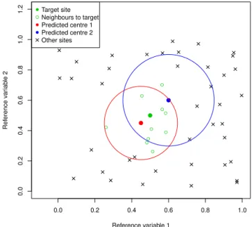
neigh-bourhood that truly regroups the most hydrologically simi-lar sites to the target location can be identified. However, in practice, this true neighbourhood is unknown. Using instead the estimate f (x0) has an effect by which some sites are
falsely suggested as more hydrologically similar than other sites. Figure 2 illustrates a region with several sites where two neighbourhoods result from the RVN method with differ-ent predicted cdiffer-entres. The target site is illustrated as a green-coloured circle and the neighbourhood is formed by the 10 nearest sites indicated by small empty circles. The other sites are designated by crosses. The red and blue neighbourhoods are delineated by circles where the radius is selected to in-clude the 10 nearest sites. The predicted centre of the red neighbourhood is closer to the target site. Consequently, it can be seen that except for one site, the same sites as the tar-get neighbourhood are included (empty circles). On the other hand, the blue neighbourhood has a predicted centre that is located further from the target site and hence a lower pro-portion of the sites truly closer to the target are found. This shows the importance of correctly predicting the neighbour-hood centres in order to identify sites that are truly similar to the target site.
The errors related to prediction of the hydrological refer-ence variables suggest that the RVN method may include an additional source of uncertainty. Indeed, the same source of uncertainty is present among the sites of a neighbourhood delineated on the basis of the site characteristics (i.e. that the average of the hydrological variables in the neighbourhood is not a perfect predictor). This could be seen as an advantage of the RVN method since it directly assesses this source of uncertainty and tries to reduce it.
Steps 1–3 are the particularity of the RVN method, while the other steps are common in RFFA and are explained in Sect. 2. In the remainder of this study, step 4 uses a specific type of neighbourhood that is composed of a fixed number of the nearest sites (Eng et al., 2005; Tasker et al., 1996), but could also be constrained to the degree of the homogeneity of the neighbourhoods (Ouarda et al., 2001). Consequently, the selected gauged sites can be obtained by sortingh(i)and
keeping the desired number of sites. Notice that even though
h(i)does not exactly approximatehi, both distances will lead
to the same neighbourhoods if they preserve the ranks. Fi-nally, step 5 consists in the estimation of the flood quantiles using either the index-flood or the regression-based model.
Notice that the RVN method may be seen as a generaliza-tion of the ROI and the CCA methods in RFFA. Indeed, the
● ●
● ● ● ● ● ●
● ●
0.0 0.2 0.4 0.6 0.8 1.0
0.0
0.2
0.4
0.6
0.8
1.0
1.2
Reference variable 1
Ref
erence v
ar
iab
le 2
● ●
● ●
●
● ●
Target site Neighbours to target Predicted centre 1 Predicted centre 2 Other sites
Figure 2.Illustration of the neighbourhoods obtained by the RVN method.
ROI method corresponds to the RVN method for which all the reference variables are site characteristics. In that case, t0=f (x0) is known and PPR is not necessary in step 2.
Similarly, the CCA approach may be seen as the special case for which the reference variables are the canonical pairs in Eq. (4) and CCA is used instead of PPR to predict them in step 2.
3.2 Evaluation criteria
For the RVN method presented above, the neighbourhood sizes must be calibrated according to an objective criterion. In this regard, the leave-one-out cross-validation approach is a general strategy to assess the performance of the pre-dicted hydrological variableszi at sitei=1, . . ., n. In turn,
each gauged siteiis considered an ungauged target location. From the remaining gauged sites, predicted valuesz(i)can be
obtained without using the hydrological information at the target location. Discrepancies between the sampled and the predicted values are used to define evaluation criteria. Notice that the hydrological variables are transformedyi =g (zi).
Hence, ifyis the sample mean of theyi, then an appropriate
global performance measure is the Nash–Sutcliffe criterion:
NHS=1−
n P
i=1
yi−y(i)2
n P
i=1
yi−y
Additionally, the predictive performance is examined at the original scale by the RRMSE:
RRMSE= v u u t
1
n
n X
i=1
1−z(i) zi
2
. (11)
The choice of the reference variables is an important aspect and a set of reference variables should be chosen in order to enforce the desired properties. For instance, with the index-flood model the assumption of a regional distribution sug-gests that, apart from the index flood, the at-site distributions must be proportional to a regional distribution. A heterogene-ity measure based on the dispersion of the L coefficient of variation (LCV) is shown to be a proper way to ensure that the LCV is relatively constant (Viglione et al., 2007). Ac-cordingly, letIjbe the set of indices for theNnearest gauged
sites to the target locationj during the cross-validation pro-cess. The regional LCVθˆ(j )is calculated as the average,
ˆ θ(j )=
1
N
X
i∈Ij
θi, (12)
of the at-site LCVθi inside thejth region. The heterogeneity
measure is defined as
H(j )=
X
i∈Ij
θi− ˆθ(j ) 2
. (13)
In their procedure, Hosking and Wallis (1997) used this heterogeneity measure to test for regional homogeneity, which implies that the regional LCV can be considered con-stant. Hence, the result of this test allow us to decide if a re-gion must be divided into smaller and more homogenous sub-regions. In the present study, the size of the neighbourhoods is the same. Hence, if a homogeneity test is performed with a given neighbourhood size, some of the neighbourhoods will be considered homogenous, while the others will be consid-ered heterogeneous (Das and Cunnane, 2011). However, the heterogeneity measure in Eq. (13) remains a useful indicator of dispersion for the regional LCV θˆ(j ) inside a
neighbour-hood. Consequently, a smallerH(j )suggests that the regional
LCVθˆ(j )is measured with less uncertainty.
To facilitate the interpretation of the results and to ensure the comparability between neighbourhoods, the heterogene-ity measureH(j )/Nis considered instead. The measure
rep-resents the sample variance of the LCV for thejth target lo-cation. This heterogeneity measure is standardized byH /n, whereHis the heterogeneity measure in Eq. (13) calculated on all n available gauged sites. The resulting ratio corre-sponds to a scale-free heterogeneity measure, where a value under one provides evidence of a less heterogeneous neigh-bourhood in comparison to the whole data set. Therefore, the average heterogeneity measure (AHM) criterion below is de-fined as the average of every neighbourhood considered in
the cross-validation process:
AHM= 1
N·H
n X
j=1
H(j ). (14)
This criterion is not specific to a given target location, but represents the global level of heterogeneity resulting from a given delineation method, such as ROI, CCA or RVN. In particular, a delineation method with a smaller AHM is an indication that, on average, a more precise regional LCV is used to predict flood quantiles.
Another desired property for a neighbourhood is that it leads to estimation models with less uncertainty. For the index-flood model, this implies in particular less uncertainty in the prediction of the index flood, while for regression-based models, it implies less uncertainty in the prediction of flood quantiles. For a multiple regression model, the uncer-tainty can be quantified by the residual variance:
s(j )2 = 1 N
X
i∈Ij
ei,(j )2, (15)
whereei,(j ) is the residual at theith gauged site, when
pre-dicting thejth target location in the cross-validation process. Notice that a regression model fitted on two different neigh-bourhoods (for the same target location) can obtain identical values, but can lead to different levels of uncertainty. In this study, a neighbourhood with a smaller residual variance is said to be relatively more efficient.
During the cross-validation process, the sample variance of the regression models can be calculated for every site, which leads to the average relative efficiency (ARE) criterion defined by
ARE=ns12 n X
j=1
s(j )2 , (16)
where the residual variances2is calculated from the multi-ple regression model on the whole data set. This criterion is similar to the AHM criterion as it is standardized to a scale-free measure. This criterion can be used to identify the de-lineation method which achieves, on average, the smallest residual variances for each neighbourhood. The ARE and the AHM criteria are used in the present study, along with the NHS and RRMSE to access the performances of the various models.
4 Application 4.1 Data
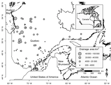
of 100 years, denoted as Q100. The analysis is performed on 151 sites located in the southern part of the Province of Québec, Canada. Figure 3 illustrates the location of these sites. Each site has at least 15 years of data, and the aver-age record length is 31 years. The usual hypotheses of sta-tionarity, homogeneity and independence are verified for all 151 data series. Only a brief description of the data and the at-site frequency analysis is provided since the elements were already presented in detail in previous studies (e.g. Chok-mani and Ouarda, 2004).
The at-site distributions are selected among several fam-ilies including generalized extreme values (GEVs), Pearson type III (P3), generalized logistic (GLO) and log-normal with three parameters (LN3). In general, the estimation of the at-site distribution was achieved by maximum likelihood and the final choices of distributions are based on the Akaike information criterion. Recent studies on the same data set have identified four relevant site characteristics (Chebana et al., 2014; Durocher et al., 2015), which are used in the present analysis: the drainage area or BV (km2), the fraction of the basin area occupied by lakes or PLAC (%), the an-nual mean liquid precipitation or PLMA (mm) and the lon-gitude or LON. Proper transformations are applied to these site characteristics in order to obtain approximately standard normal distributions.
4.2 Determination of the neighbourhood centres Steps 1–2 of the RVN method represent the selection of the reference variables and, if necessary, the estimation of the hy-drological reference variables at the target locations. Two ini-tial groups of reference variables are considered and updated by backward step-wise selection. The first group is based on L-moments only and the second is based on the combination of L-moments and site characteristics. The acronym LM for L-moment and HYB for hybrid are used to identify the two groups. More precisely, the L-moments considered for both groups are the sample average (L1), the LCV, the L coef-ficient of skewness (LSK) and the L coefcoef-ficient of kurtosis (LKT). These reference variables are transformed and stan-dardized to obtain zero mean and unit variance. The transfor-mation used for L1 and LCV is the logarithm, while for LSK and LKT, the transformation is log(x−mx+1), wheremxis
the minimum of the reference variables.
A specific implementation of PPR is assumed, which con-siders the smooth functionsgkin Eq. (8) as cubic spline
poly-nomials with five equally spaced knots. The number of knots is validated by cross validation using the NHS criterion. No-tice that for the fitting of LSK, one site has a very low stan-dardized residual of approximately −6. Consequently, this site is considered an outlier and removed from the estimation of the reference variables. In previous studies (e.g. Chokmani and Ouarda, 2004), this site was identified as one of a few problematic sites that are difficult to predict due to an under-estimated drainage area or over-evaluated percentage of area
Figure 3. Location of the 151 hydrometric stations in southern Québec, Canada.
covered by lakes. Nevertheless, in the present study, this site is removed only during the prediction of the reference vari-ables and all sites are included in the rest of the analysis.
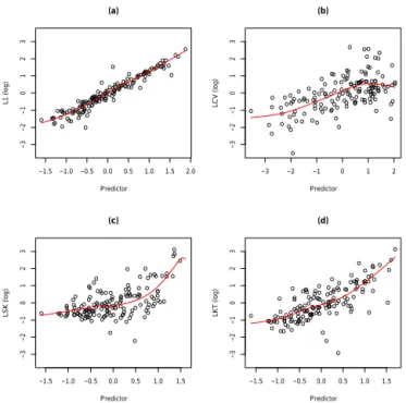
Figure 4 shows the fitting of the four reference variables by the PPR models. Cross validation has selected PPR mod-els with a unique directionαfor all reference variables. The PPR equations that describe the relation between the refer-ence variables and the site characteristics are explicit; for in-stance, the regression equation for the LCV has the form log(LCV)= −1.80+0.26×f
−0.67×log(BV)−0.09
×√PLAC+1.27×log(PLMA)+0.06×LON−1.32i. (17) Notice the constant term −1.32 and the norm of direction
|α| 6=1 inside the functionf in Eq. (17). The difference be-tween Eq. (17) and the general form of the PPR model in Eq. (9) is the consequence of transformations on the explana-tory variables. Indeed, during the optimization procedure of a PPR model, it is suggested to scale the explanatory variables in order to avoid the scale effect in the coefficients of the di-rectionα(Hastie et al., 2009). Nevertheless, it is important to notice that the formula inside the functionf corresponds to a linear model.
val-● ● ● ● ● ● ● ● ● ● ● ● ●● ● ● ● ● ● ● ● ●●● ● ● ● ● ● ● ● ● ● ● ● ● ● ● ● ● ● ● ● ● ● ● ● ● ● ● ● ● ● ● ● ● ●●● ● ● ● ● ● ● ● ● ● ● ● ● ●● ● ● ● ● ● ● ● ● ● ● ● ● ● ● ● ● ●● ● ● ● ● ● ● ● ● ● ● ●● ● ● ● ● ● ● ● ● ● ● ● ● ● ● ● ● ● ● ● ● ● ● ● ●● ● ● ● ● ● ● ● ● ● ● ● ● ● ●● ● ● ● ● ● ● ● ●
−1.5 −1.0 −0.5 0.0 0.5 1.0 1.5 2.0
−3 −2 −1 0 1 2 3 (a) Predictor L1 (log) ● ● ● ● ● ● ● ● ● ● ● ● ●● ● ● ● ● ●● ● ● ● ● ● ● ● ● ●● ● ● ● ● ● ● ● ● ● ●● ● ● ●● ● ● ● ● ● ● ● ● ● ● ● ● ● ● ● ● ● ● ● ● ● ● ● ● ● ● ● ● ● ● ●● ● ● ● ● ● ● ● ● ● ● ● ● ● ● ● ● ● ● ● ● ● ●● ● ● ● ● ● ● ● ● ● ● ● ● ● ● ● ● ● ● ● ● ● ● ● ● ● ● ● ● ● ● ● ● ● ● ● ● ● ● ● ● ● ● ● ● ● ● ● ● ● ● ●
−3 −2 −1 0 1 2
−3 −2 −1 0 1 2 3 (b) Predictor LCV (log) ● ● ● ● ● ● ● ● ● ● ● ● ● ● ● ● ● ● ● ● ● ● ● ● ● ● ● ● ● ● ● ● ● ● ● ● ● ● ● ● ● ● ● ● ● ● ● ● ● ● ● ● ● ● ● ● ● ● ● ● ● ● ● ● ● ● ● ● ● ● ● ● ● ● ● ● ● ● ● ● ● ● ● ● ● ● ● ● ●● ● ● ● ● ● ● ● ● ● ● ● ● ● ● ● ● ● ● ● ● ● ● ● ● ● ● ● ● ● ● ● ● ● ● ● ●● ● ● ● ● ● ● ● ● ● ● ●● ● ● ● ● ● ● ● ● ● ● ●
−1.5 −1.0 −0.5 0.0 0.5 1.0 1.5
−3 −2 −1 0 1 2 3 (c) Predictor LSK (log) ● ● ● ● ● ● ● ● ●● ●● ● ● ● ● ● ● ● ●● ● ● ● ● ● ● ● ● ● ● ● ● ● ● ● ● ● ● ● ● ● ● ● ● ● ● ● ● ● ● ● ● ● ● ● ● ● ● ● ● ● ● ● ● ● ● ● ● ● ● ●● ● ● ● ● ● ● ● ● ● ● ● ● ● ● ● ● ● ● ●● ● ● ● ● ● ● ● ● ● ● ● ● ● ● ● ● ● ● ● ● ● ● ● ● ● ● ● ● ● ● ● ● ● ● ● ● ● ● ● ● ● ● ● ● ● ● ● ● ● ● ● ● ● ● ● ● ● ●
−1.5 −1.0 −0.5 0.0 0.5 1.0 1.5
−3 −2 −1 0 1 2 3 (d) Predictor LKT (log)
Figure 4.Residuals of the reference variables by PPR methods.
ues of the NHS criterion: 90.9, 28.2, 7.8 and 48.1 %, respec-tively. Notice that the NHS criterion is calculated by cross-validation; consequently, even though the improved perfor-mances by the PPR method appear moderate they represent true fitting improvements.
Due to its poor fit, LSK may not be a proper reference variable for the delineation step. To validate this assumption, the neighbourhoods are formed with and without using LSK and the rest of the analysis is carried out for both scenarios. Based on the RRMSE criterion, LSK must be maintained, as it is associated with better predictive performances. This strategy is part of the backward step-wise selection procedure as described in Sect. 3.1. Overall, it leads to discarding LKT and to maintaining L1, LCV and LSK. The second group of reference variables contains both the L-moments and the site characteristics. As with the first group, backward step-wise selection is performed and the final reference variables are BV, PLAC, LCV and LSK. In order to distinguish the two groups of reference variables, RVN-LM will designate the first group with the L-moments only and RVN-HYB will designate the second group with both the L-moments and the site characteristics.
4.3 Results of the index-flood model
At this point, the steps 1–4 of the RVN methodology are per-formed and the neighbourhoods are identified. Notice that for the RVN-LM method, the reference variables include the first three L-moments, which could be used as a moment estima-tor to deduce the target distribution. This approach is, how-ever, not generally applicable to the present methodology as
the reference variables are selected by a step-wise procedure. Moreover, it is necessary to identify a proper family of dis-tributions from regional information, which is achieved here by analysing the distribution of the gauged sites inside the neighbourhoods. The index-flood model and the L-moments algorithm were proven to lead to a reliable procedure to iden-tify a regional distribution and to estimate its parameters (Hosking and Wallis, 1997). In this model, the regional quan-tile corresponding to a return periodrat a target locationiis writtenQi(r)=µiQ(r), whereµi is the index flood. In the
present study, the index flood is taken to be the means of the at-site distributions and is predicted at the target location by multiple regression.
The index-flood model is fitted inside the neighbourhoods obtained by each one of the four methods: ROI, CCA, RVN-LM and RVN-HYB. For CCA, two canonical pairs are calcu-lated using flood quantiles corresponding to the 10- and 100-year return periods as hydrological variables, as described in Sect. 2.1. The choice of the regional distribution is made be-tween the four common families of distributions that were mentioned earlier: GEV, GLO, LN3 and P3. The parameters of the regional quantile functionQ (r) are calculated from the regional LCV and the regional LSK as the respective av-erages (see Eq. 12). Figure 5a shows the L-moment ratio di-agram for the regional LSK and LKT with RVN-LM. For each neighbourhood, the distribution family is selected as the one having the nearest regional LKT to the theoretical value, given the regional LSK. RVN-HYB is omitted in Fig. 5 to im-prove the clarity of the illustration, but has similar behaviour to RVN_LM.
Figure 5b, c and d present the L-moment ratio diagrams of the at-site LCV and LSK for three given target locations as an illustration of the gauged sites found in the respective neighbourhoods. In these diagrams, the nearest gauged sites selected for RVN-LM, CCA and ROI are highlighted. Fig-ure 5b shows that RVN_LM has a denser cluster of gauged sites in terms of LCV and is approximately centred on the true target. Conversely, Fig. 5c and d show situations where the true targets do not correspond to the predicted target. Al-though, all the reference variables are known at the target location for the ROI method, Fig. 5b and c show that the se-lected sites are not located around the true target. This finding is consistent with the results of GREHYS (1996a, b) which indicates that delineation according to physiographical sim-ilarity can lead to substantially different regions than delin-eation according to hydrological similarity.
0.05 0.10 0.15 0.20
0.12
0.14
0.16
0.18
(a)
LSK
LKT
GEV P3 GLO LN3 + + +
+
+
+ +
+
+ + ++ + + +
+
+ +
+
+ +
+ + +
+ + +
+ ++
+ + +
+ +
+ +
+ +
+ +
+
+ + +
+
+
+ ++ +
+ + +
+
+
+ +
+ + + + +
+
+ +
+ + +
+
+ + ++ + ++
+ +
+
+ +
+ +
+
+ +
+
++ +
+ + +
+
+ +
+ +
+ +
+ +
+ + +
+ +
+ +
+
+ +
+
+ +
+
+ +
+
+ +
+
+ + +
+ +
+
+ +
+
+
+ +
+
+ + + + +
+ +
+
++ + + +
+ +
0.05 0.10 0.15 0.20 0.25 0.30
−0.2
0.0
0.1
0.2
0.3
0.4
0.5
(c)
LCV
LSK
●
0.05 0.10 0.15 0.20 0.25 0.30
−0.2
0.0
0.1
0.2
0.3
0.4
0.5
(b)
LCV
LSK
●
0.05 0.10 0.15 0.20 0.25 0.30
−0.2
0.0
0.1
0.2
0.3
0.4
0.5
(d)
LCV
LSK
●
●Target ROI CCA RVN_LM
Figure 5.L-moments ratio diagram for index-flood model.(a)
Re-gional L-moments for RVN-LM with 29 gauged sites.(b, c, d)
Re-gional L-moments based on the 15 nearest gauged sites for 3 se-lected target locations.
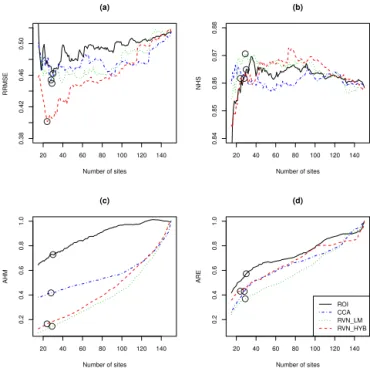
NHS is achieved with nearly 80 sites. Nevertheless, the op-timal values for the three other methods are obtained with approximately 30 sites for both criteria. Figure 6b indicates that all methods have a relatively stable NHS between 86 and 87 %, but the best NHS is obtained by RVN-LM. Con-versely, Fig. 6a shows clearer improvements of the calibra-tion in terms of the RRMSE criterion. Hence, the calibrated models are set according to the RRMSE criterion and are rep-resented by circles in Fig. 6. The results are summarized in Table 1. RVN-HYB, with a RRMSE of 40.1 %, outperforms the other methods. In particular, a difference of 6.1 and 5.3 % is observed, respectively, with the traditional ROI and CCA methods.
Figure 6c and d present, respectively, the AHM and the ARE criteria obtained from the considered methods. The AHM criterion indicates that the ROI and the CCA meth-ods have lower heterogeneity than the whole data set in gen-eral, but are largely outperformed by the LM and RVN-HYB methods especially for smaller neighbourhoods. This is not surprising as the RVN-LM and RVN-HYB pool to-gether sites with similar L-moments, but this quantifies the intuitive assumption that the regional LCV is calculated with less uncertainty when the L-moments are directly considered instead of other reference variables. In particular, the AHM of the ROI method is 72.8 % with the optimal neighbour-hood size of 30. In comparison, the AHM of the RVN-LM method is 14.5 % with the optimal neighbourhood size of 29 sites, which is considerably lower. Figure 6c shows that
20 40 60 80 100 120 140
0.38
0.42
0.46
0.50
(a)
Number of sites
RRMSE
● ●●
●
20 40 60 80 100 120 140
0.84
0.85
0.86
0.87
0.88
(b)
Number of sites
NHS
● ● ●
●
20 40 60 80 100 120 140
0.2
0.4
0.6
0.8
1.0
(c)
Number of sites
AHM
●
●
● ●
20 40 60 80 100 120 140
0.2
0.4
0.6
0.8
1.0
(d)
Number of sites
ARE ●
● ● ●
ROI CCA RVN_LM RVN_HYB
Figure 6.Evaluation criteria for the index-flood model. Calibrated models are represented by circles.
the AHM criterion of the RVN-LM method does not reach a similar level to the ROI method until as many as 120 sites are used. These results indicate that even for relatively small neighbourhoods, the ROI method identifies regions that are only slightly less hydrologically heterogeneous than all sites pooled together. This suggests that, in the present case study, the ROI method has difficulties identifying sites that are sim-ilar to the target site in terms of LCV.
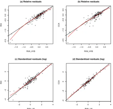
As mentioned in Sect. 4.2, previous studies have identified a few problematic stations in the considered data set. Figure 7 presents the residuals between different methods. As it may be difficult to see small improvements by uniquely observ-ing points around they=xlines, the visualization of Fig. 7 is improved by adding a flexible fit of the point cloud, using a standard smoothing spline approach. The resulting red lines indicate, if close tox, that the residuals are lower on average for one of the two methods. In general, the points associated with the largest relative discrepancies are close to they=x
line, which indicates that the sites that are difficult to predict are essentially the same for all methods. However, Fig. 7a and b show that the RVN-HYB method specifically improves the prediction of the sites with the lowest and largest rela-tive discrepancies as the red line is clearly located under the
Table 1.Evaluation criteria for the RVN method for optimal neighbourhood sizes.
Model Size RRMSE NHS AHM ARE
Index flood
ROI 30 46.2 86.5 72.8 57.3
CCA 28 45.4 86.2 41.7 42.9
RVN-LM 29 45.0 87.1 14.5 36.9
RVN-HYB 24 40.1 86.2 16.5 43.1
Regression based
ROI 30 44.9 86.9 72.8 64.7
CCA 28 43.5 86.1 41.7 30.6
RVN-LM 39 41.7 87.6 17.9 39.8
RVN-HYB 24 39.5 86.2 16.5 42.5
Best criteria is written in bold.
+ + + + + + + ++ + + + + + ++ + + + + + + + + + + + + ++ + + + + + + + + + + + + + + + + + + + ++ + + ++ + ++ + + + + + + + + + ++ + + + + + + ++ + + + + + + + + + + + + + + ++ + + + + + + + + + + + + + + + + + + + + + + + + + + + + + + ++ + + + + + + + + + + + + + + + ++ + + ++ + + + + +
−1.5 −1.0 −0.5 0.0 0.5
−2.5
−1.5
−0.5
0.0
0.5
(a) Relative residuals
RVN_HYB R OI + + + + + + + ++ + + ++ + + + ++ + + + + + + + + ++ ++ + + ++ + + + + + + + +++ + + + + + ++ + + + + + ++ + + + + + + + + + ++ + + + + + + + + + + + + + + + + + + + + + + + + + + + + + + + + + + + + +++ + + + + + + + + + + + + + + + +++ + + + + + + + + + + + + + + ++ + + + + + + + + +
−1.5 −1.0 −0.5 0.0 0.5
−2.5
−1.5
−0.5
0.0
0.5
(b) Relative residuals
RVN_HYB CCA + + + + + + + + + + + + + + + + ++++ + + + + + + + + + + + + + ++ + + + + + + + ++ + + + + + + ++ + + + ++ + + + + + + + + + + + + + + + + + + ++ ++ + + + + + + + + + + ++ + + + ++ + + + + + + + + + + + + + + + + + + + + + + + + + + + + + + + + + + + + + + + + + + + + + + + + + + + + + + +
−2 0 2 4
−4
−2
0
2
(c) Standardized residuals (log)
RVN_LM
R
OI ++
+ + + + + ++ + + + + + + + ++++ + + + + + + + + + + + + + ++ + + + + + + +++ + + + + + + + + + + ++ + + + + + + + + + + + + + + + + + + + + + + + + + + + + + + + + + ++ + + + ++ + + + + + + + + + + + + + + + + + ++ + + + + ++ + + + + ++ + + + + + + + + + + + + + + + + + + + + + + + +
−2 0 2 4
−4
−2
0
2
(d) Standardized residuals (log)
RVN_LM
CCA
Figure 7. Comparison of the cross-validation residuals for Q100 for different methods. The black line is the unitary slope and the red line is a smooth fitting of the residuals.
The present case study is an example of a region where some sites are problematic for any method. In practice, the residuals are not known; consequently, we do not know if the target sites of interest will be problematic or not. Globally, what Fig. 7a indicates is that the RVN-HYB model is some-how more robust, because for the sites that are well predicted by simpler models, such as ROI, RVN-HYB will perform similarly on average. However, if the target site is predicted less accurately, the RVN-HYB model will (on average) be better in terms of RRMSE. Consequently, the overall gain may seem of moderate magnitude. However, for some prob-lematic stations, the gain could be more substantial. In par-ticular, the red lines in the left part of Fig. 7a appear mostly
20 40 60 80 100 120 140
0.38
0.42
0.46
0.50
(a)
Number of sites
RRMSE
● ●
●
●
20 40 60 80 100 120 140
0.84 0.85 0.86 0.87 0.88 (b)
Number of sites
NHS
●
● ●
●
20 40 60 80 100 120 140
0.0 0.2 0.4 0.6 0.8 1.0 (c)
Number of sites
AHM
●
●
● ●
20 40 60 80 100 120 140
0.0 0.2 0.4 0.6 0.8 1.0 (d)
Number of sites
ARE ● ● ● ● ROI CCA RVN_LM RVN_HYB
Figure 8.Evaluation criteria for the regression-based model. Cali-brated models are represented by circles.
influenced by two points, but the two improvements are of 77.2 and 68.5 %, which is considerable.
4.4 Results of the regression-based model
Prediction of Q100 at the target location is also carried out by the regression-based model using the same delineation meth-ods as with the index-flood model, but with potentially dif-ferent calibration values for the neighbourhood sizes. Conse-quently, the descriptions of steps 1–4 (in Sect. 3.1) are identi-cal to those of the index-flood approach and are not repeated here.
RRMSE. Although all methods differ by less than 2 % in terms of NHS, results indicate that NHS values ing to CCA and RVN-HYB are inferior to those correspond-ing to the regression model applied to all gauged sites, which corresponds ton=150 in Fig. 8b. However, CCA leads to the best relative efficiency as indicated by the ARE criterion in Table 1. Hence, CCA corresponds to the regression mod-els with, on average, the lowest uncertainties. This indicates that flood quantiles may be better reference variables for the regression-based model than for the index-flood model and suggests that, in general, different reference variables may be more appropriate for different situations. Nevertheless, the two close lines in Fig. 8d reveal that, for the same neigh-bourhood size, the RVN-LM method has ARE values that are similar to CCA. In terms of AHM, Fig. 8c is identical to Fig. 5c, except that new neighbourhood sizes are indicated in circles.
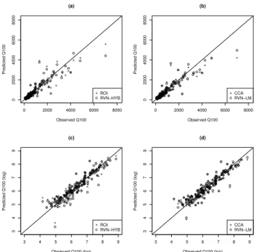
The fit of the regression-based model is graphically as-sessed in Fig. 9 by quantile–quantile plots. It is shown that, for all the delineation approaches, the regression-based mod-els correctly predict the flood quantile Q100 at target loca-tions, as it correctly follows the y=x line. However, the comparison between the methods ROI and RVN-HYB shown in Fig. 8a, c and the methods CCA and RVN-LM shown in Fig. 8b, d do not show clear differences. A more precise as-sessment would be obtained by comparing the residuals in-stead, as it is done in Fig. 7. However, the predictions of the regression-based models are very similar to those of the index-flood models and they will lead to very similar figures, which are not reported here. Table 1 also provides a compari-son of the performance of the index-flood and the regression-based models. In terms of RRMSE and NHS criterion, the two approaches will lead to very similar results, which is consistent with what it is reported in other studies (GRE-HYS, 1996a, b; Haddad and Rahman, 2012). Therefore, sim-ilar conclusions can be drawn from the two approaches. For instance, in both cases, the RVN-HYB method leads to the best results in terms of RRMSE.
5 Conclusions
A general methodology was investigated to improve ho-mogenous properties of neighbourhoods in RFFA. A proce-dure to calculate relevant reference variables at a target lo-cation prior to the RFFA was proposed to improve neigh-bourhood properties and to reduce uncertainties. The pre-dicted values of reference variables represent the unknown centres of neighbourhoods delineated according to a distance of gauged sites with respect to the centres. The proposed method represents a generalization of both ROI and CCA methods in RFFA. The proposed RVN method has the ad-vantage of accepting various groups of reference variables, considering nonlinear interrelations and being more
objec-+ + + + + + + + + ++ ++++ ++ + + + + +++ + + + + + + +++ + ++ + +++++ + + + + + ++ + + + ++ + + ++ + + + + + ++ +++++++++ + + + ++ + +++++++++++++++ + + + + + + ++ + +++ + + + + + + + + + + + + + + + + + + + + + + + + + + + + + ++++ + + + + + + + + + + +
0 2000 4000 6000 8000
0 2000 4000 6000 8000 (a) Observed Q100 Predicted Q100 ● ● ● ● ● ● ● ● ● ●●●●● ● ●● ● ● ● ● ●●● ● ● ● ● ● ● ● ● ● ● ●● ● ●●●●● ● ● ● ● ● ●● ● ● ● ● ● ● ● ●●● ● ● ● ● ● ● ● ●●●●● ●●● ●● ● ● ● ● ● ● ●● ● ● ● ● ● ●● ●● ●● ● ● ● ● ● ● ●● ● ●●● ● ● ● ● ● ● ● ● ● ● ● ● ● ● ● ● ● ● ● ● ● ● ● ● ● ● ● ● ● ●●●● ● ● ● ● ● ● ● ● ● ● ● + oROIRVN−HYB
+ + + ++ + + + + ++ ++++ +++ ++++++ + + + + + + ++++ ++ + +++++ + + + + + ++ + + + ++ + + ++ + + + + + ++ +++++++++ ++ + + + + ++ ++++++++++++++ + + + + + + + + +++ + + + + + + + + + + + + + + + + + + + + + + + + + + + + + ++++ + + + + + + + + + + +
0 2000 4000 6000 8000
0 2000 4000 6000 8000 (b) Observed Q100 Predicted Q100 ● ● ● ● ● ● ● ● ● ●●● ● ● ● ●● ● ● ● ● ●●● ● ● ● ● ● ● ● ● ● ● ●● ● ●●●●● ● ● ● ● ● ●● ● ● ● ● ● ● ● ●●● ● ● ● ● ● ● ● ●●●●●●●● ●● ● ● ● ● ● ● ●●● ● ● ● ● ●● ●● ● ● ● ● ● ● ● ● ●● ● ●● ● ● ● ● ● ● ● ● ● ● ● ● ● ● ● ● ● ● ● ● ● ● ● ● ● ● ● ● ● ● ●●●● ● ● ● ● ● ● ● ● ● ● ● + oCCARVN−LM
+ ++ + + + + + ++ + + + + + + + + + + + + + + + + + + + + + + + + + + + + + + + + + + + + + + + + + + + + + + +++ + + + + + + + + + + + + + + + + + + + + + + + + + + + + + +++ + + + + + + + + + + + + + + + + + + + + + + + + + + + + + + + + + + + + + + + + + + + + + + + + + + + + + + + + + + + +
3 4 5 6 7 8 9
3 4 5 6 7 8 9 (c)
Observed Q100 (log)
Predicted Q100 (log)
● ●● ● ● ● ● ● ●● ● ● ● ● ● ● ● ● ● ● ● ● ● ● ● ● ● ● ● ● ● ● ● ● ● ● ● ● ● ● ● ● ● ● ● ● ● ●● ● ● ● ● ● ● ● ●● ● ● ● ● ● ● ● ● ● ● ● ● ● ●● ● ●● ● ● ● ● ● ● ● ● ● ● ● ● ● ●● ● ● ● ● ● ● ● ● ● ● ● ● ● ● ● ● ● ● ● ● ● ● ● ● ● ● ● ● ● ● ● ● ● ● ● ● ● ● ● ● ● ● ● ● ● ● ● ●● ● ●● ● ● ● ● ● ● ● ● + oROIRVN−HYB
+ + + + + + + + ++ ++ + + + + + + + + + + + + + + + + + + + + + + + + + + + + + + ++ + + + ++ + + + + + + + +++ + + + + + + + + + + + + ++ + ++ + + + + + + + + + + + + ++ + + + + + + + + + + + + + + + + + + + + + + + + + + + + + + + + + + + + ++ + + + + + + + + + + + + + ++ + + + + + + + +
3 4 5 6 7 8 9
3 4 5 6 7 8 9 (d)
Observed Q100 (log)
Predicted Q100 (log)
● ●● ● ● ● ● ● ● ● ● ● ● ● ● ● ● ● ● ● ● ● ● ● ● ● ● ● ● ● ● ● ● ● ● ● ● ● ● ● ● ● ● ● ● ● ● ●● ● ● ● ● ● ● ● ● ● ● ● ● ● ● ● ● ● ● ● ● ● ● ●● ● ●● ● ● ● ● ● ● ● ● ● ● ● ● ● ●● ● ● ● ● ● ● ● ● ● ● ● ● ● ● ●● ● ● ● ● ● ● ● ● ● ● ● ● ● ● ● ● ● ● ● ● ● ● ● ● ● ● ● ● ● ● ● ●● ● ●● ● ● ● ● ● ● ● ● + oCCARVN−LM
Figure 9.Quantile–quantile plot of Q100 for the RVN method with the regression-based model.
tive since L-moments are used instead of estimated flood quantiles from at-site analysis.
In this study, the reference variables correspond to trans-formed L-moments. The resulting RVN-LM and RVN-HYB methods were applied to sites located in the southern part of the province of Québec, Canada, to predict flood quantiles corresponding to the 100-year return period by both index-flood and regression-based models. The prediction of the ref-erence variables at target locations showed that, after proper transformations, L1 can be linearly related to the site char-acteristics, but no proper transformations are found for the other L-moments. This justifies the consideration of the PPR method to account for the nonlinearity in the prediction of the reference variables. In general, other models, such as gen-eralized additive models or artificial neural networks, could be considered instead of PPR to account for the nonlinear-ity. Nevertheless, the PPR approach unveils direction vectors that provide explicit, parsimonious and meaningful regres-sion equations.
CCA and RVN methods has reduced the uncertainty on the regional LCV, the index flood and the predicted flood quan-tiles, in comparison to ROI. Consequently, prior modelling of hydrological reference variables was shown to be advan-tageous for the delineation of neighbourhoods in RFFA.
The present study has made specific assumptions in order to investigate the RVN method in well-defined conditions. Nevertheless, the approach that consists in predicting hydro-logical reference variables in an a priori analysis remains valid when other choices of regression models, neighbour-hood forms and metrics are considered. More comparative studies should be carried out to evaluate alternatives to fixed size neighbourhoods and Euclidian distances in the specific context of the RVN framework.
The L coefficient of skewness is commonly used in RFFA to describe the shape of a distribution. Consequently, to im-prove the result of the RVN method, further research efforts could focus on improving the prediction of this crucial refer-ence variable. One way to improve the prior analysis of the hydrological reference variables is the consideration of the unequal sampling error. This aspect is often considered in the estimation of flood quantiles in RFFA, but may also play an important role in the prior analysis of the RVN method.
6 Data availability
The raw hydrological data can be obtained from the En-vironment Ministry of the Province of Quebec (http:// www.mddelcc.gouv.qc.ca/), and the raw meteorological data can be obtained directly from the website of Environment Canada (http://climate.weather.gc.ca/).
Acknowledgements. Financial support for this study was gra-ciously provided by the Natural Sciences and Engineering Research Council (NSERC) of Canada. The authors are grateful to the editor, Elena Toth, and the two reviewers whose comments and suggestions contributed to the improvement of the manuscript.
Edited by: E. Toth
Reviewed by: T. Gado and one anonymous referee
References
Bishop, C. M.: Neural networks for pattern recognition, Oxford University Press, Oxford, UK, 1995.
Burn, D. H.: An appraisal of the “region of influence” ap-proach to flood frequency analysis, Hydrol. Sci. J. 35, 149–166. doi:10.1080/02626669009492415, 1990.
Castiglioni, S., Castellarin, A., and Montanari, A.: Prediction of low-flow indices in ungauged basins through physio-graphical space-based interpolation, J. Hydrol., 378, 272–280, doi:10.1016/j.jhydrol.2009.09.032, 2009.
Chebana, F. and Ouarda, T. B. M. J.: Multivariate L
-moment homogeneity test, Water Resour. Res., 43, W08406, doi:10.1029/2006WR005639, 2007.
Chebana, F. and Ouarda, T .B. M. J.: Depth and homogeneity in regional flood frequency analysis, Water Resour. Res., 44, W11422, doi:10.1029/2007WR006771, 2008.
Chebana, F. and Ouarda, T. B. M. J.: Index flood-based multivariate regional frequency analysis, Water Resour. Res., 45, W10435, doi:10.1029/2008WR007490, 2009.
Chebana, F., Charron, C., and Ouarda, T. B. M. J., and Mar-tel, B.: Regional frequency analysis at ungauged sites with the generalized additive model, J. Hydrometeorol., 15, 2418–2428, doi:10.1175/JHM-D-14-0060.1, 2014.
Chokmani, K. and Ouarda, T. B. M. J.: Physiographical space-based kriging for regional flood frequency estimation at ungauged sites, Water Resour. Res., 40, W12514, doi:10.1029/2003WR002983, 2004.
Cunderlik, J. M. and Burn, D. H.: Switching the pooling similarity distances: Mahalanobis for Euclidean, Water Resour. Res., 42, W03409, doi:10.1029/2005WR004245, 2006.
Cunnane, C.: Methods and merits of regional flood frequency anal-ysis, J. Hydrol., 100, 269–290, 1988.
Dalrymple, T.: Flood-frequency analysis, Geological Survey Water-Supply Paper 1543, 80 pp., 1960.
Das, S. and Cunnane, C.: Examination of homogeneity of selected Irish pooling groups, Hydrol. Earth Syst. Sci., 15, 819–830, doi:10.5194/hess-15-819-2011, 2011.
Dawson, C. W., Abrahart, R. J., Shamseldin, A. Y., and Wilby, R. L.: Flood estimation at ungauged sites us-ing artificial neural networks, J. Hydrol., 319, 391–409, doi:10.1016/j.jhydrol.2005.07.032, 2006.
Durocher, M., Chebana, F., and Ouarda, T. B. M. J.: A Nonlin-ear Approach to Regional Flood Frequency Analysis Using Pro-jection Pursuit Regression, J. Hydrometeorol., 16, 1561–1574, doi:10.1175/JHM-D-14-0227.1, 2015.
Eng, K., Tasker, G. D., and Milly, P.: An Analysis of Region-Of-Influence methods for flood regionalization in the Gulf-Atlantic rolling plain, J. Am. Water Resour. As., 41, 135–143, doi:10.1111/j.1752-1688.2005.tb03723.x, 2005.
Friedman, J. H. and Tukey, J. W.: A projection pursuit algorithm for exploratory data analysis, IEEE T. Comput., 100, 881–890, 1974.
Friedman, J. H., Grosse, E., and Stuetzle, W.: Multidimensional Ad-ditive Spline Approximation, SIAM J. Sci. Stat. Comp., 4, 291– 301, doi:10.1137/0904023, 1983.
GREHYS: Presentation and review of some methods for re-gional flood frequency analysis, J. Hydrol., 186, 63–84, doi:10.1016/S0022-1694(96)03042-9, 1996a.
GREHYS: Inter-comparison of regional flood frequency procedures for canadian rivers, J. Hydrol., 186, 85–103, doi:10.1016/S0022-1694(96)03043-0, 1996b.
Griffis, V. and Stedinger, J.: The use of GLS regression in regional hydrologic analyses, J. Hydrol., 344, 82–95, 2007.
Hastie, T., Tibshirani, R., and Friedman, J. H.: The elements of sta-tistical learning: data mining, inference, and prediction, Springer Series in Statistics, Springer, New York, doi:10.1007/978-0-387-84858-7, 2009.
He, Y., Bárdossy, A., and Zehe, E.: A review of regionalisation for continuous streamflow simulation, Hydrol. Earth Syst. Sci., 15, 3539–3553, doi:10.5194/hess-15-3539-2011, 2011.
Hosking, J. R. M. and Wallis, J. R.: Regional frequency analysis: an approach based on L-moments, Cambridge University Press, Cambridge, UK, 1997.
Hwang, J.-N., Lay, S.-R., Maechler, M., Martin, R. D., and Schimert, J.: Regression modeling in back-propagation and pro-jection pursuit learning, IEEE T. Neural. Networ., 5, 342–353, doi:10.1109/72.286906, 1994.
Kjeldsen, T. R. and Jones, D. A.: An exploratory analysis of error components in hydrological regression modeling, Water Resour. Res., 45, W02407, doi:10.1029/2007WR006283, 2009. Laio, F., Ganora, D., Claps, P., and Galeati, G.: Spatially smooth
re-gional estimation of the flood frequency curve (with uncertainty), J. Hydrol., 408, 67–77, doi:10.1016/j.jhydrol.2011.07.022, 2011. Ouali, D., Chebana, F., and Ouarda, T. B. M. J.: Non-linear canon-ical correlation analysis in regional frequency analysis, Stoch. Env. Res. Risk A., 30, 449–462, doi:10.1007/s00477-015-1092-7, 2015.
Ouarda, T. B. M. J.: Regional flood frequency modeling, Chapter 77, in: Chow’s Handbook of Applied Hydrology, 3rd Edn., edited by: Singh, V. P., Mc-Graw Hill, New York, 77.1–77.8, 2016. Ouarda, T. B. M. J. and Shu, C.: Regional low-flow frequency
anal-ysis using single and ensemble artificial neural networks, Water Resour. Res., 45, W11428, doi:10.1029/2008WR007196, 2009. Ouarda, T. B. M. J., Haché, M., Bruneau, P., and Bobée,
B.: Regional Flood Peak and Volume Estimation in North-ern Canadian Basin, J. Cold Reg. Eng., 14, 176–191, doi:10.1061/(ASCE)0887-381X(2000)14:4(176), 2000. Ouarda, T. B. M. J., Girard, C., Cavadias, G. S., and Bobée,
B.: Regional flood frequency estimation with canonical corre-lation analysis, J. Hydrol., 254, 157–173, doi:10.1016/S0022-1694(01)00488-7, 2001.
Ouarda, T. B. M. J., Ba, K. M., Diaz-Delgado, C., Carsteanu, A., Chokmani, K., Gingras, H., Quentin, E., Trujillo, E., and Bobee, B.: Intercomparison of regional flood frequency estimation meth-ods at ungauged sites for a Mexican case study, J. Hydrol., 348, 40–58, doi:10.1016/j.jhydrol.2007.09.031, 2008.
Pandey, G. R.: Assessment of scaling behavior of regional floods, J. Hydrol. Eng., 3, 169–173, doi:10.1061/(ASCE)1084-0699(1998)3:3(169), 1998.
Pandey, G. R. and Nguyen, V.-T.-V.: A comparative study of regres-sion based methods in regional flood frequency analysis, J. Hy-drol., 225, 92–101, doi:10.1016/S0022-1694(99)00135-3, 1999. Reis, D., Stedinger, J., and Martins, E.: Bayesian generalized least squares regression with application to log Pearson type 3 regional skew estimation, Water Resour. Res., 41, W10419, doi:10.1029/2004WR003445, 2005.
Stedinger, J. and Lu, L.-H.: Appraisal of regional and index flood quantile estimators, Stoch. Hydrol. Hydraul., 9, 49–75, 1995. Stedinger, J. and Tasker, G.: Regional hydrologic analysis: 1.
Or-dinary, weighted, and generalized least squares compared, Water Resour. Res., 21, 1421–1432, doi:10.1029/WR021i009p01421, 1985.
Tasker, G., Hodge, S., and Bark, S.: Region of Influence re-gression for estimating the 50-year flood at ungaged sites, J. Am. Water Resour. As., 32, 163–170, doi:10.1111/j.1752-1688.1996.tb03444.x, 1996.
Viglione, A., Laio, F., and Claps, P.: A comparison of homogene-ity tests for regional frequency analysis, Water Resour. Res., 43, W03428, doi:10.1029/2006WR005095, 2007.