www.atmos-chem-phys.net/17/1/2017/ doi:10.5194/acp-17-1-2017
© Author(s) 2017. CC Attribution 3.0 License.
A missing source of aerosols in Antarctica – beyond long-range
transport, phytoplankton, and photochemistry
Michael R. Giordano1,a, Lars E. Kalnajs2, Anita Avery1, J. Douglas Goetz1, Sean M. Davis3,4, and Peter F. DeCarlo1,5
1Department of Civil, Architectural, and Environmental Engineering, Drexel University, Philadelphia, Pennsylvania, USA 2Laboratory for Atmospheric and Space Physics, University of Colorado at Boulder, Boulder, Colorado, USA
3Chemical Sciences Division, NOAA Earth System Research Laboratory, Boulder, Colorado, USA
4Cooperative Institute for Research in Environmental Sciences, University of Colorado at Boulder, Boulder, Colorado, USA 5Department of Chemistry, Drexel University, Philadelphia, Pennsylvania, USA
anow at: AAAS Science and Technology Fellowship, Hosted at US Environmental Protection Agency, Washington DC, USA
Correspondence to:Peter F. DeCarlo ([email protected])
Received: 10 July 2016 – Published in Atmos. Chem. Phys. Discuss.: 14 July 2016 Revised: 3 November 2016 – Accepted: 4 November 2016 – Published: 2 January 2017
Abstract. Understanding the sources and evolution of aerosols is crucial for constraining the impacts that aerosols have on a global scale. An unanswered question in atmo-spheric science is the source and evolution of the Antarctic aerosol population. Previous work over the continent has pri-marily utilized low temporal resolution aerosol filters to an-swer questions about the chemical composition of Antarctic aerosols. Bulk aerosol sampling has been useful in identify-ing seasonal cycles in the aerosol populations, especially in populations that have been attributed to Southern Ocean phy-toplankton emissions. However, real-time, high-resolution chemical composition data are necessary to identify the mechanisms and exact timing of changes in the Antarctic aerosol. The recent 2ODIAC (2-Season Ozone Depletion and Interaction with Aerosols Campaign) field campaign saw the first ever deployment of a real-time, high-resolution aerosol mass spectrometer (SP-AMS – soot particle aerosol mass spectrometer – or AMS) to the continent. Data obtained from the AMS, and a suite of other aerosol, gas-phase, and mete-orological instruments, are presented here. In particular, this paper focuses on the aerosol population over coastal Antarc-tica and the evolution of that population in austral spring. Results indicate that there exists a sulfate mode in Antarctica that is externally mixed with a mass mode vacuum aerody-namic diameter of 250 nm. Springtime increases in sulfate aerosol are observed and attributed to biogenic sources, in agreement with previous research identifying phytoplankton activity as the source of the aerosol. Furthermore, the
to-tal Antarctic aerosol population is shown to undergo three distinct phases during the winter to summer transition. The first phase is dominated by highly aged sulfate particles com-prising the majority of the aerosol mass at low wind speed. The second phase, previously unidentified, is the generation of a sub-250 nm aerosol population of unknown composi-tion. The second phase appears as a transitional phase during the extended polar sunrise. The third phase is marked by an increased importance of biogenically derived sulfate to the total aerosol population (photolysis of dimethyl sulfate and methanesulfonic acid (DMS and MSA)). The increased im-portance of MSA is identified both through the direct, real-time measurement of aerosol MSA and through the use of positive matrix factorization on the sulfur-containing ions in the high-resolution mass-spectral data. Given the importance of sub-250 nm particles, the aforementioned second phase suggests that early austral spring is the season where new particle formation mechanisms are likely to have the largest contribution to the aerosol population in Antarctica.
1 Introduction
2007), and sulfur compounds (Legrand et al., 1988; Mul-vaney et al., 1992) in Antarctic ice cores has been used to provide information on glaciation, sea level, cloudiness, and volcanic activity over the past millennia. Aerosols also play a major role in Earth’s current climate due to their im-pact on the global radiative balance and cloud microphysics. Unfortunately, aerosols are still the least understood and constrained aspects of the climate system (Boucher et al., 2013). The uncertainty of aerosols’ climate impacts arises from the fact that how an aerosol affects the radiative bal-ance is a function of both an aerosol’s chemical composition and physical properties (e.g., size, shape). Both the chemi-cal and physichemi-cal properties of aerosols are functions of emis-sion sources, atmospheric processing, and lifetime in the at-mosphere. Over recent decades, much work has been done to characterize aerosol emission sources and background aerosol across much of the globe (Boucher et al., 2013), but there are difficulties in assessments of preindustrial to present-day forcing. Measurements in Antarctica, provide in-sight into one of the more pristine environments and can be useful in the understanding of preindustrial background aerosol (e.g., Hamilton et al., 2014). However, the ability to sample pristine aerosols is directly related to an area’s inac-cessibility. Because of the difficulty in performing science in Antarctica, the Antarctic aerosol mass and number popula-tion (particularly its sources and evolupopula-tion) is still a subject of many open questions in atmospheric science. Improving our understanding of the processes that govern aerosol for-mation and evolution in Antarctica is important not only to our understanding of present-day Antarctica, but also to un-derstanding the broader climate history.
Besides a few research stations, bases, and minor tourism activities, anthropogenic emission sources of aerosols and trace gases are rare in and around Antarctica (Shirsat and Graf, 2009). Much of the work produced over the years examining Antarctic aerosols has been done precisely be-cause of the lack of direct anthropogenic atmospheric in-fluences. Multiple investigations of the concentration, size distribution, spatial distribution, and composition of Antarc-tic aerosols have been performed over various parts of the continent (e.g., Shaw, 1979; Lechner et al., 1989; Harwey et al., 1991; Savoie et al., 1993; Hara et al., 1996; Minikin et al., 1998, Koponen et al., 2003). Low time-resolution bulk aerosol analysis (generally filter-integrated) dominates the chemical composition measurements over the continent (e.g., Prospero et al., 1991; Wagenbach, 1996; Minikin et al., 1998; Preunkurt et al., 2007) though real-time measurement tech-niques have been deployed in recent years (e.g., Belosi et al., 2012).
The results of aerosol measurements over Antarctica over the past decades have been generally consistent on two major points: that a persistent, low concentration, aerosol popula-tion exists over the entirety of the continent and that sulfate is a major component of that aerosol, especially in the aus-tral spring and summer (Shaw, 1979; Parungo et al., 1981;
Wagenbach et al., 1988). On a global scale, anthropogenic sources of sulfur dominate the sulfate aerosol mass which has long been known to be a major component of aerosol-induced climate forcing (Charlson et al., 1987, 1990; Kul-mala et al., 2002). However, in the Southern Hemisphere, and particularly in Antarctica, biogenic sources are thought to be the largest source of sulfur to the atmosphere (Bates et al., 1992; Carslaw et al., 2010, and references therein). Hence, the question of the origin of the Antarctic aerosol sulfate arises. Globally, volcanic activity provides a major source of atmospheric sulfur so the presence of Mt Erebus (78◦S), the
southernmost active volcano, should be noted. However, iso-topic studies have shown that, in Antarctica, sulfate of vol-canic origin is of minimal importance although infrequent, short-lived exceptions – due to eruptions – have occurred (Patris et al., 2000). The descent of stratospheric sulfur into the lower atmosphere is another potential sulfur source but has also been shown to be a minor source of sulfate around coastal Antarctica (Legrand and Wagenbach, 1998). The two most likely remaining origins of sulfur are ocean sea-spray and non-sea-spray marine sources.
Marine sulfur appears in both primary and secondary aerosols. Primary marine aerosols, generally referred to as sea-spray aerosols, are produced through mechanical ac-tions such as wave breaking and bubble bursting. Sea-spray aerosols are mostly super-micron in size and production is a strong function of wind speed (Lewis and Schwartz, 2004). The super-micron sea-spray aerosol is dominated by sea salt, of which sulfate is 8 % by weight in ocean water. In Antarc-tica, previous measurements have placed sea salt as 50–80 % by mass of the (sub-10 µm) aerosol population depending on the time of year (Weller et al., 2008). Marine secondary aerosols, however, are driven by biological emissions of volatile organic compounds. Of these compounds, dimethyl sulfide (DMS) and its oxidation product methanesulfonic acid (MSA) are the most common and account for 75 % of the global biogeochemical sulfur cycle (Chasteen and Bent-ley, 2004). In Antarctica, enhancements in sulfate-to-sodium ratios (over the seawater ratio) in aerosols have been at-tributed to DMS and MSA. Off-line measurement and calcu-lation of non-sea-spray (nss-) sulfate have been used to iden-tify seasonal cycles of aerosol sulfate fractions over Antarc-tica (e.g., Prospero et al., 1991; Wagenbach, 1996; Minikin et al., 1998; Preunkurt et al., 2007). Spring and summertime en-hancements in phytoplankton activity in the Southern Ocean provide an excellent explanation for the spring sulfate aerosol enhancements seen over Antarctica (Gibson et al., 1990; Ari-moto et al., 2001; von Glasow and Crutzen, 2004; Preunkert et al., 2007; Read et al., 2008; Weller et al., 2011a). Un-fortunately, non-sea-spray sulfate has generally been calcu-lated using aerosol sodium concentrations. Because sodium is nonconservative in Antarctic aerosols due to mirabilite (Na2SO4×10H2O) precipitation in sea ice microstructures,
DMS have been conducted over inland Antarctica (Concor-dia Station), but without real-time aerosol measurements, it is impossible to determine the actual impact of marine biota on Antarctic sulfate (Preunkert et al., 2008).
Beyond sulfate and chemical composition information in general, knowledge of aerosol physical properties is neces-sary to constrain their climate effects. For example, quanti-fying the ability of aerosols to form cloud droplets is one of the key challenges in determining the overall climate effects of aerosols. This could be of particular importance in the Antarctic where cloud formation may be limited by the low concentration of aerosols available to act as cloud condensa-tion nuclei (CCN). Determining the CCN spectrum of a given aerosol population is possible once the size distribution, size-resolved composition, and mixing state of the aerosol popu-lation is known (Petters and Kreidenweis, 2007; Wang et al., 2010). Mixing state is one of the more difficult to measure properties of the aerosol spectrum. The extremes of mixing state are termed internal mixtures (all particles in a popu-lation, regardless of size, have identical chemical composi-tions) or external mixtures (there are multiple particle popu-lations with distinct and differing compositions) though most real aerosol populations are somewhere in between (Textor et al., 2006). The mixing state of an aerosol population af-fects cloud forming predictions when the aerosol population is comprised of components of significantly differing hygro-scopicities (Wex et al., 2010). Because Antarctic aerosols seem to primarily be composed of sulfates and salts, the ef-fect of the mixing state on cloud forming predictions may be minimized over the continent itself but overestimated as continental air masses flow out over the Southern Ocean and gain organic components.
The recent field campaign 2ODIAC – 2 Season Ozone De-pletion and Interaction with Aerosols Campaign – deployed a set of instruments that can begin to answer some of the out-standing questions about Antarctic aerosols, in particular, the questions surrounding high time-resolution chemical specia-tion to determine the sources of the aerosol mass populaspecia-tion. This is the first paper from the campaign and focuses on the sources of Antarctic (coastal) aerosols and the physical prop-erties of the sulfate aerosol mass population.
2 Methods 2.1 Field site
The 2ODIAC campaign took place over 2 years with mea-surements occurring during the austral spring–summer of 2014 (October–December) and the austral winter–spring of 2015 (August–October). A field site was set up on the sea ice in McMurdo Sound approximately 20 km from Mc-Murdo Station, Antarctica. The 2014 field site was located at 77◦41′40′′S, 166◦11′58′′E, while the 2015 site was 5 km
away at 77◦42′58′′S, 166◦24′30′′E. The dynamic nature of
sea ice prevented the collocation of the field sites over both field seasons. However, the 2015 site was chosen such that the wind fetch was similar to the fetch from the 2014 site. In 2014, the field site was located approximately 16 km away from the sea ice edge as compared to approximately 8 km away in 2015.
In both field seasons, the field sites consisted of 2 struc-tures (“fish huts”). One structure housed the atmospheric sampling instrumentation, while the other housed a 5 kW diesel generator. The generator hut was placed 75 m to the southwest of the instrumentation hut because at both field sites the wind blew primarily from the northwest and south-east. The distance between and orientation of the huts en-sured that minimal self-sampling occurred over both field seasons. During low-wind periods and certain wind shifts, self-sampling and sampling of McMurdo did occur, but these periods were identified and removed from the data via careful observation of NOx and aerosol mass spectrometer (AMS)
data. The thresholds in regard to self-contamination were ap-plied if (a) a rapid increase in NOxand associated decrease in
ozone and (b) the organic signal in the AMS at combustion-relevantm/z(e.g.,m/z57 or 55) increased by greater than 20 %.
2.2 Instrumentation
Atmospheric sampling instrumentation for both seasons con-sisted of a suite of aerosol and gas-phase instruments. The gas-phase suite was composed of an ozone monitor (1 s time resolution; Thermo Environmental model 49C) and an NOx
monitor (1 s time resolution; Thermo Environmental model 42C). The aerosol suite consisted of aerosol sizing instru-ments, an aerosol concentration counter, aerosol composition measurements, and aerosol collectors. In 2014, aerosol sizing was carried out via a scanning electrical mobility spectrom-eter (∼9 to 850 nm; 2 min time resolution; Brechtel Man.
Inc.; SEMS) and an ultra-high sensitivity aerosol spectrom-eter (∼55 to > 1000 nm; 1 s time resolution; Droplet Meas.
Tech.; UHSAS). In 2015, aerosol sizing was carried out via a scanning mobility particle sizer (∼10 to 420 nm; 2 min
and 2015 deployments, respectively (Jayne et al., 2000). The inlet for the aerosol sampling line was covered and heated to prevent sampling of windblown snow and to prevent riming, respectively. At the flow conditions and geometry of the sam-pling inlet, transmission of < 1 µm particles to the AMS was > 95 %. Overall, the aerosol inlet system had a 50 % trans-mission efficiency at 5 µm and 0 % transtrans-mission efficiency of particles > 9 µm. All transmission efficiency values are as calculated by a particle loss calculator using the specific ge-ometry of the setup (von der Weiden et al., 2009). This work focuses primarily on results from the aerosol size, concentra-tion, and composition instruments. Future work will discuss results from other parts of the instrumentation suite, includ-ing the particle filters and snow samples.
Meteorological data were recorded by a colocated weather station (Davis Vantage Pro2). The anemometer (rated 0– 200 km h−1), temperature and relative humidity probes (3◦C
and 3 % accuracy, respectively), and solar radiation sensors (spectral response 400–1100 nm, 1 Wm−2 resolution,±5 %
accuracy at full scale) were mounted on a pole 50 m NE of the sampling hut. It should be noted that, due to the sensitiv-ity and accuracy of the radiometers, solar irradiance is pre-sented in this paper as an approximate value. These values are useful to separate different temporal periods in the data but should not be taken as indicative of actinic flux values. Data from the sensors was wirelessly transmitted to the con-trol unit located in the instrumentation hut.
During both field seasons, all of the instruments were rou-tinely calibrated and, where applicable, verified against each other. For 1 h each day, at different times every day, the inlet was switched to a HEPA filter for all of the particle instru-ments. This daily period allowed for a background signal to be calculated for the AMS and ensured no part of the in-let system was leaking (via monitoring of the particle coun-ters/sizers). In depth calibrations and checks were conducted weekly. For the AMS, the weekly calibration included an ion-ization efficiency calibration using ammonium nitrate (atom-ized and size selected via the SEMS or SMPS at 300 nm) and a particle time-of-flight (PToF) size calibration using PSL (polystyrene latex; 60, 100, 300, 600, and 800 nm). Across both field seasons, the AMS calibrations changed by less than 10 % while in the field. To check the particle counters against each other, ammonium nitrate was size selected by the SEMS or SMPS and the output measured by the associated CPCs and EPC. Weekly zeros and spans were also conducted for the gas analyzers.
3 Results and discussion
Figure 1 shows the records for wind speed, wind direction, number concentration from the EPC, and sulfate concen-tration from the AMS for both 2ODIAC field seasons. The wind speed, wind direction, and particle number concentra-tion traces were collected every second but have been
aver-aged to 2 min records to match the AMS data recording rate. The time series is displayed with the 2015 field season as the leftmost part of thex axis to emphasize inter-seasonal transitions – from winter to spring (2015) and spring to sum-mer (2014).
Figure 1a shows the wind direction (degrees) as a func-tion of time and colored as a funcfunc-tion of wind speed (m s−1),
for both seasons. The 2015 field season (winter–spring) was dominated by winds coming from the ESE with high wind speeds. Over 80 % of the entire 2015 field season had wind coming from the ESE. Additionally, more than 60 % of the 2015 field season had wind speeds recorded at over 8 m s−1.
By contrast, the 2014 field season (spring–summer) wind fetch had a more bimodal wind direction distribution and an opposite wind speed probability distribution as compared to 2015. In 2014, the wind direction distribution was 60/40 % ESE/NW and was above 8 m s−1for only 20 % of the
sea-son. These meteorological patterns and seasonal differences are not unusual for this region (Seefeldt et al., 2003).
Figure 1b shows the number concentration from the EPC over both field seasons. The figure shows the 2 min average as well as a 1 h average. With total condensa-tion nuclei (CN) number concentracondensa-tions ranging between 50–1000 cm−3, 2ODIAC’s observations are consistent with
other coastal and interior Antarctic field measurements (e.g., Jaenicke et al., 1992; Gras, 1993; Koponen, et al., 2003; Be-losi et al., 2012). Figure 1b shows a major facet of Antarc-tic aerosols: that there is a steady-state aerosol concentration during calm and low-wind periods. The steady-state concen-trations here are defined as the concenconcen-trations at which 99 % of the recorded data is over. During the 2015 field season aerosol number concentrations were at a minimum of near 50 cm−3at the start of the campaign (early September). As
the season progressed and the sun began to rise in the aus-tral spring, the background concentration of aerosols rose to 125 cm−3. The 2014 field season experienced a similar
min-imum of approx. 75 cm−3 but did not see the same rise in
the background aerosol number population. Dotted lines at these values are included on Fig. 1b to aid the eye. A lack of combustion-derived organic aerosol signal in the AMS and the persistence of these particles independent of wind direc-tion suggests that the background aerosol is neither a result of local pollution (e.g., our own generators or vehicles) nor transported pollution from McMurdo.
Figure 1c shows the aerosol sulfate concentration mea-sured by the AMS over the course of both field seasons. Aerosol sulfate positively tracks with the total aerosol counts both in the wind speed dependence and the trends in back-ground concentrations. In 2015, total aerosol sulfate begins the season (in early September) at 20 ng m−3and rises to
ap-prox. 40 ng m−3as solar irradiance begins increasing at the
end of September. In 2014, total aerosol sulfate increases from approx. 30 ng m−3 (in October) to 60 ng m−3 (in
1000
800
600
400
200
0
Particle number
concentration
(no.
cm
-3 )
9/11 9/21 10/1 10/11
Austral spring (2015)
10/31 11/10 11/20 11/30
Austral summer (2014) 100
80
60
40
20
0
Sulfate concentration
(ng m
-3 )
300
200
100
0
Wind direction
(deg)
25 20 15 10 5 0
Wind speed (m s )
-1
(a)
(b)
(c)
Figure 1.For both the 2014 and 2015 field seasons, with 2015 on the left:(a)wind direction record colored as a function of wind speed,
displayed as a 2 min average record (standard deviation 0.2 m s−1and 2◦);(b)2 min (light blue; standard deviation of 11 and 18 cm−3for 2015 and 2014, respectively) and 1 h (black) records of particle number concentration from the EPC;(c)2 min records of sulfate concentration from the aerosol mass spectrometer. Dotted lines in(b)indicate the minimums in particle number concentrations (99th percentile) measured over the field seasons.
well documented. The values reported here are 2–3 times less than previous aerosol sulfate measurements in coastal Antarctica (Minikin et al., 1998; Rankin and Wolff, 2003). However, the previous measurements are filter-integrated as-sessments from Antarctic bases other than McMurdo (e.g., Halley, Neumayer, Dumont d’Urville) with differing size ranges and sampling techniques. Without coincident mea-surements across the continent, it is difficult to determine if spatial or temporal factors are responsible for the differences in concentrations between literature values of aerosol sulfate and the presented values.
While aerosol sulfate is the main focus of this paper, it is not the only aerosol component and the relative amount of sulfate measured by the AMS should be contextualized. Over both field seasons, sulfate generally makes up more than 50 % of the total mass of the traditionally reported non-refractory species (organics, sulfate, nitrate, and ammo-nium). Both the absolute amount and relative percentage of total non-refractory mass of sulfate are higher in 2014 than 2015. Ammonium, organics, and nitrate, in that order, make up the rest of the non-refractory species measured by the AMS. When adding measurements of refractory Na and Cl to the non-refractory species (as discussed in a forthcoming paper, Giordano et al., 2016), sulfate is the third most abun-dant species at 5–30 % of the total submicron aerosol mass.
3.1 Sulfate aerosols as an external mixture
1.4
1.2
1.0
0.8
0.6
0.4
0.2
0.0
Arbitrary units
2 3 4 5 6 7 8 9
100 2 3 4 5 6 7 8 91000 2
PToF size (nm)
ESE, low wind ESE, med. wind ESE, high wind
NW, low wind NW, med. wind NW, high wind
Figure 2.AMS PToF results of AMS sulfate for 2014 as functions
of wind speed (solid lines (> 8 m s−1) vs. dotted lines (2–8 m s−1 and < 2 m s−1)) and wind direction (black (northwest) vs. red (east– southeast)). The PToF mass has been arbitrarily scaled to enhance readability of the figure. The PToF results for 2015 are identical in both distribution shape and peak location for all wind regimes.
vacuum aerodynamic diameter distributions from the AMS for the 2014 field season as a function of wind speed and direction. Regardless of where an air mass originated, the sulfate aerosol as measured by the AMS exhibited a well-distributed mode centered at a vacuum aerodynamic diameter of approximately 250 nm. This result is consistent with pre-vious ocean-based size measurements of subantarctic MSA-containing aerosol (250 and 370 nm from Zorn et al., 2008, and Schmale et al., 2013, respectively) as well as off-line filter-integrated measurements in coastal Antarctica (200– 350 nm aerodynamic diameter impactor stage; Jourdain and Legrand, 2001). None of the other species measured in the AMS showed a well-defined size mode.
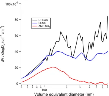
Similar to the AMS, the size distributions from the other aerosol sizing instruments were consistent across wind di-rection regimes as long as conditions conducive to blow-ing snow events (here defined as wind speeds greater than 8 m s−1)are excluded. Figure 3 shows the average size
dis-tributions from the UHSAS, SEMS, and AMS from the 2014 field season when blowing snow events are excluded. For Fig. 3, all three measurements have been converted to a vol-ume equivalent diameter to allow intercomparisons of the three different methods of aerosol sizing by applying the fol-lowing assumptions: (1) a density of 1.8 g cm−3for the
sul-fate aerosol population; (2) sphericity of all aerosols in the population; (3) equality of the optical diameter from the UH-SAS and volume equivalent diameter (DeCarlo et al., 2004). As evidenced by the sizing instruments, the sulfate distribu-tion is well encompassed by both the UHSAS and SEMS.
100 x10-3
80
60
40
20
0
dV / dlogD
p
(um
3 cm
-3 )
5 6 7 8 9
100 2 3 4 5 6 7
Volume equivalent diameter (nm) UHSAS
SEMS AMS SO4
Figure 3.Average dV /dlogDpas a function of volume equivalent
diameter for low and medium wind speeds of 2014. Results of the particle time of flight of the sulfate species from the AMS (red) are shown with the SEMS (black) and UHSAS (blue).
For 2015 (not shown), the result is the same with the SMPS distribution compared to the AMS PToF. Without the size-resolved sulfate distribution from the AMS, it would not be possible to identify the externally mixed mode that is present. The presence of an external mixture has implications both for estimating the bulk direct radiative forcing of Antarc-tic aerosol and for predicting CCN number concentrations (NCCN)in the Antarctic troposphere. Many atmospheric ra-diation and global climate models assume external mixtures of aerosols (Koch et al., 2006; Bauer et al., 2007). Incorrectly assuming an externally mixed aerosol can result in incor-rectly estimating radiative forcing by a factor of 3 or more (Bauer et al., 2007; Kim et al., 2008). Recent improvements to radiative forcing models have focused on incorporating internally mixed aerosol populations (Boucher et al., 2013). The results presented here, although limited in seasonal cov-erage and duration of sampling, suggest that radiative forc-ing models for Antarctica should continue to treat the sulfate mass population as an external mixture. This work does sup-port the assumptions of older estimates of radiative forcing for sulfate aerosols over Antarctica of approx.−0.1 Wm−2
(Myhre et al., 1998). It should be noted that the appearance of sulfate primarily at the lower end of the size distributions of Antarctic aerosol does not preclude the presence of sul-fate in larger or smaller particles. The aerodynamic lens of the AMS inlet system precludes measurements of particles larger than 1µ.
With regard to NCCN, though size-resolved composition
al., 2007). A simple volume-weighted mixing rule such as the Zdanovskii–Stokes–Robinson relationship (ZSR, Stokes and Robinson, 1966) or the equivalent Kappa formulation (Petters and Kreidenweis, 2007) is used to determine particle hygroscopicity. If non-size-resolved data from the AMS are used, the mixing rule implicitly assumes an internally mixed aerosol mass population and can bias calculated hygroscop-icity high or low. In general, internal mixtures dominate aerosol populations as the distance from the emission source increases, and the mixing rule is an appropriate assumption, regardless of the individual emission sources (e.g., Juranyi et al., 2010; Garbariene et al., 2012). However, when close to emission sources (especially anthropogenic sources), ex-ternal mixtures are generally observed (Kander and Schultz, 2007; Swietlicki et al., 2008; Wex et al., 2010). The results here, however, are an externally mixed aerosol number pop-ulation. The results presented here suggest that the Antarctic aerosol population may be a special case: despite a large dis-tance between open water (presumably the major source of breaking waves near Antarctica) and the coast, an externally mixed aerosol population is persistent over the continent. Generally, there exists in the atmosphere enough mass to condense on pre-existing particles, which reduces the impact of external mixtures downwind of the sources. Alternatively, these results may suggest that open water is unnecessary for large ocean–atmosphere aerosol fluxes and that sea ice or other sources could be a dominant source of coastal Antarc-tic aerosol number population. The results presented here are limited by the fact that 2ODIAC occurred only on the sea ice, but the consistency of these results in context of the liter-ature suggests that, at the least, they apply over a wider area of coastal Antarctica. It should be noted that previous studies in Antarctica that have measuredNCCNhave reported exter-nally mixed CCN populations. Unfortunately, previous work has been conducted at Palmer Station or around the Antarctic Peninsula areas which have a strong and consistent marine influence (DeFelice, 1996; O’Dowd et al., 1997). This pre-vious work has been unable to remove the marine influence from the continental air masses. An externally mixed sulfate mode, as this work demonstrates, appears to be a unique and ubiquitous feature of Antarctic aerosols. Calculating NCCN
is not within the scope of this paper but will be presented in future publications on 2ODIAC.
3.2 Sulfate as a predominant component of the background Antarctic aerosol number population If the externally mixed sulfate mode observed in the AMS is, in fact, the primary component of the background aerosol concentration, then some degree of closure between the EPC number concentration and the AMS PToF data should be possible. Again assuming particle sphericity and an aver-age material density of 1.8 g cm−3 for sulfate (an average
value between sulfuric acid and ammonium sulfate), the total number of sulfate particles can be calculated from the
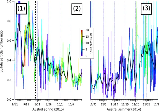
size-resolved sulfate mass distribution in the AMS PToF mode measured over the entirety of the campaign. This process assumes sphericity of particles, takes the mass distribution measured in vacuum aerodynamic diameter space, and using the density value transforms it to volume vs. volume equiv-alent diameter for that sulfate mode, which can then be con-verted into a number distribution and integrated to find the to-tal number of particles from the measured sulfate mass distri-bution. Figure 4 shows the ratio of the total number of sulfate particles calculated from the measured AMS sulfate size dis-tribution (average PToF size disdis-tribution scaled to the high-resolution sulfate mass concentrations) to the total number of particles measured in the EPC. This number distribution cal-culation is assuming no counter ion to the measured sulfate, i.e., the sulfate is present as sulfuric acid, which is consistent with previous Southern Ocean data (Zorn et al., 2008). As in Fig. 1a, the 2014 and 2015 field seasons have been com-bined and the data trace is colored by wind speed in meters per second.
As discussed in the forthcoming Kalnajs et al. (2016) pub-lication, higher wind speeds increase the non-sulfate aerosol counts. In discussing the background aerosol number popu-lation, any occurrence of blowing snow (implemented in this paper roughly as wind speeds above 8 m s−1, as suggested
by Li and Pomeroy, 1997) should therefore be ignored. For Fig. 4, this roughly translates to ignoring non-blue/green sec-tions of the record. The total record is produced here for com-pleteness, but Fig. 4 also includes a smoothed trace (boxcar smoothing) that excludes high wind speed events (since high wind speeds and particle counts are strongly correlated, to be discussed in a forthcoming paper, Giordano et al., 2016).
Sulfate modes can be described as three distinct phases as shown in Fig. 4 (indicated by numbers and vertical lines). First, in the late austral winter–early spring, sulfate com-prises the majority of the total aerosol counts – often over 60 % (1). Second, the percent of the total aerosol number population that is made up of sulfate, then takes a sharp de-cline (2). Third, the percent sulfate gradually climbs again as the austral spring transitions to summer (3). The spring– summer increase is primarily evident in the 2014 data. While the fraction of particles that are primarily sulfate has a dis-tinct cycle during these three phases, it should be empha-sized that the sulfate mass is steadily increasing from winter to summer (Fig. 1c).
1.0
0.8
0.6
0.4
0.2
0.0
Sulfate particle number ratio
9/11 9/16 9/21 9/26 10/1 10/6
Austral spring (2015)
10/31 11/5 11/10 11/15 11/20 11/25 11/30
Austral summer (2014)
(1)
(2)
(3)
20
15
10
5
0
Wind speed (m s )
-1
Figure 4.Sulfate number ratio as calculated from the AMS PToF mode divided by the total number concentration from the EPC over both
2014 (right) and 2015 (left). Both field seasons’ data are colored by recorded wind speeds. A smoothed trace of only wind speeds < 8 m s−1 is overlaid in black. Rough timing for the phases discussed in Sect. 3.2 are noted.
has not previously been identified as a major aspect of the annual evolution of the Antarctic aerosol number population. We note that this transitional season has only been observed in this dataset, and future observational datasets measured during this period are important for understanding the con-sistency of this period.
Phase 2 is consistent with measuring newly formed parti-cles that have been transported to our measurement location during a transitional period during the extended Antarctic sunrise. Throughout this paper, all instances of “new particle formation” refer to a regional, not local, growth of previously unobserved aerosol mass unless otherwise noted. The parti-cles that are formed during this transitional period make up a significant fraction of the total aerosol number concentration at the very start of the austral spring. The new aerosol pop-ulation’s contribution to the total Antarctic number popula-tion, however, decreases as biogenic emissions in the South-ern Ocean increase.
The exact cause of Phase 2 is difficult to determine from the instrumentation deployed during 2ODIAC, but poten-tial explanations can be narrowed down. From Fig. 1 during Phase 2, both the total counts on the EPC and the sulfate mass in the AMS trend upward. However, total counts increases faster than the mass captured in the AMS. Three possible ex-planations therefore exist for the trends seen in Fig. 4 during Phase 2:
1. The particles are refractory and would not be measured by the AMS regardless of size,
2. the particles are being counted in the AMS but are not sulfate (e.g., organics, nitrate), or
3. there are particles measured by the EPC that are either not producing a measurable size distribution signal or outside of the AMS measurement range at either the low (less than∼40 nm) or the high end (greater than 1µ). These three explanations for the transitional aerosol num-ber population observed in Phase 2 must be examined before any conclusions on the source(s), impacts, or fate of the new number population can be drawn. A thorough discussion of these three possibilities is found in Appendix B, but the main points are discussed here.
is impossible to rule out. The reader is again referred to Ap-pendix B for a complete discussion, but the measurements from the sizing instruments (SMPS and SEMS) and AMS suggest that the transitional aerosol is equal to or less than 250 nm in (vacuum aerodynamic) diameter. Unfortunately, given the instrumentation deployed, it is impossible to de-termine the composition of these very small particles (e.g., less than 100 nm) due in part to the low mass loadings inher-ent in Antarctica and the effects that low mass loadings have on AMS PToF data.
The potential sources of the transitional aerosol population
Phases 2 and 3 suggest that the photochemical processes af-fecting the Antarctic and Southern Ocean aerosol popula-tions undergo at least two distinct phases. Unfortunately, de-termining the driving force behind either phase is not pos-sible with the data available nor are there much data in the literature to explain the existence of phases 2 and 3. For ex-ample, though the springtime MSA-derived aerosol increase has long been measured in Antarctica, data regarding what threshold of sunlight is necessary for the sulfate increase has been lacking. Data on Southern Ocean chlorophyll concen-trations, light requirements for phytoplankton photosynthe-sis, and even solar irradiance measurements during Antarctic aerosol campaigns are sparse. During 2ODIAC, however, so-lar irradiance at the field site was measured for both field sea-sons though the values presented here should, again, be seen as approximate and indicative of a transitional period in the aerosol number population. The percentage of sulfate parti-cles declines to a minimum of 20 % when solar irradiance av-erages between 100 and 200 Wm−2(i.e., most of the austral
spring after the sun had (partly) risen over McMurdo Sound). In the late spring–early summer transition, where daily peak solar irradiance averages well over 300 Wm−2, the
percent-age of sulfate aerosol begins to increase again.
Taken in conjunction with the sulfate data presented in Fig. 1 and the < 40 nm/total data in the Supplement, Fig. 4 shows that during some transitionary periods, measured dur-ing 2ODIAC as bedur-ing between 100 and 300 Wm−2, newly
formed particles (and transport to the measurement site) may generate additional particles in the Antarctic number popula-tion. This Phase 2 to Phase 3 evolution of Antarctic aerosol has not previously been observed. Given the particle com-position measurements, it is possible that significant con-tributions from non-sulfate (e.g., non-DMS related) aerosol formation mechanisms contribute to the Phase 2 aerosol. A likely explanation for the source of the new particles is the existence of some reservoir species that is photoactive dur-ing the early austral sprdur-ing. One likely reservoir species can-didate for aerosol enhancement are halogens. Much work has recently been performed examining the importance of halo-gens and solar irradiance in coastal Antarctica. Gas-phase concentrations of IO and BrO have been shown to track well
with solar irradiance levels at∼300 Wm−2 (Saiz-Lopez et
al., 2007). Solar photooxidation of frozen iodine-containing solutions has been shown to increase gas-phase iodine con-centrations as well (Kim et al., 2016). Halogens have long been linked to ozone depletion events (ODEs), and ODEs are linked to aerosol enhancements (e.g., Kalnajs et al., 2013). Unfortunately, the data are still unclear on whether the spa-tially and temporally invariant aerosol increase is due to ODEs as they have been classically observed in the polar re-gions. Another possible reservoir species in the Antarctic is mercury. Recent work has suggested that mercury can partic-ipate in new particle formation in the Antarctic atmosphere (Humphries et al., 2015). If reservoir species exist, then ques-tions beyond that of their origin begin to arise. The mass of the reservoir, rates of source depletion and aerosol produc-tion, and aerosol formation mechanisms are all questions that would require additional measurements to answer.
Regardless of whether the non-sulfate aerosol is related to a mechanism such as ODEs or the existence of a reservoir species, two observations are clear: first, a (likely) sub-40 nm mode of aerosols is somehow produced over coastal Antarc-tica in late winter–early spring, and, second, the importance of the sub-40 nm mode is reduced as sulfate mass in the larger aerosol modes increases in the late spring and early summer.
3.3 The source of Antarctic sulfate
Since the externally mixed sulfate mode observed in 2ODIAC makes up such a dominant fraction of the total non-refractory aerosol number population, it is important to deter-mine the source of the sulfate aerosol. As discussed, various other investigators have apportioned aerosol sulfate to either sea-spray or non-sea-spray sources usually through the use of sodium as a sea-spray marker. In addition to the problems of using sodium due to mirabilite fractionation, sodium is generally a refractory species in the AMS and not well cap-tured at the standard operating conditions of the instrument. Sodium can be well measured by the ion chromatography of filters, but the record produced has long time integrations (24 h in the case of 2ODIAC) and does not separate out wind and aerosol effects. Fortunately, the AMS is able to measure carbon–sulfur compounds in real time, which have previ-ously been tied to MSA concentrations in the marine bound-ary layer (Phinney et al., 2006; Zorn et al., 2008; Schmale et al., 2013).
80x10-3
60
40
20
0
MSA
0.6 0.5
0.4 0.3
0.2 0.1
0.0
SO4 (µg m )-3 Zorn et al. Schmale et al. This study 600
500
400
300
200
100
0
Daily high solar irradiation (W m
)-2
5x10⁻³
4
3
2
1
0
MSA
60x10-3
50 40 30 20 10 0
SO4
Figure 5.MSA vs. sulfate as measured by the AMS for both field seasons, colored by the daily high solar irradiance. 2ODIAC data are
presented with results from Zorn et al. (2008) and Schmale et al. (2013) for context. Inset is a zoomed in area showing the 2ODIAC data in higher detail.
al., 2008). Figure 5 shows the reconstructed MSA concen-tration vs. the total measured sulfate signal from the AMS, plotted for both field seasons. Also included in Fig. 5 are the data from two other field campaigns that measured Antarctic air masses with an AMS. The first is a reconstruction of total aerosol MSA (using an MSA fragmentation pattern) from a Southern Ocean cruise, adapted from Zorn et al. (2008). The second is an MSA-attributed factor reconstruction (via pos-itive matrix factorization, see below) from a stationary de-ployment of an AMS to Bird Island, adapted from Schmale et al. (2013). The 2ODIAC data in Fig. 5 are colored as a func-tion of the daily high solar irradiance measured at the field sites. As the sun reaches its approximate zenith, the MSA concentration in the AMS increases to almost 10 % of the to-tal sulfate signal in the AMS. During the late austral winter and into the early austral spring, the MSA fragment makes up less than 1 % of the total sulfate. The absolute concentra-tions of MSA and sulfate of 2ODIAC are lower than those previously reported by both Zorn et al. (2008) and Schmale et al. (2013) though the ratios of MSA to sulfate are similar across the three studies. Both of the previous measurements took place in regions where the origin of particulate sulfate was dominated by open-ocean source regions and took place in the austral summer and fall where more active DMS chem-istry is likely to occur. Lower MSA and sulfate concentra-tions during 2ODIAC are therefore not surprising given the differences in season and location as compared to the previ-ous studies. Higher MSA concentrations are likely to appear over McMurdo Sound as the sea ice recedes around the con-tinent in the austral summer (Jourdain and Legrand, 2001).
Positive matrix factorization
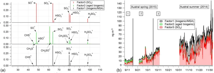
Figure 6.PMF results for the sulfur-containing species observed over both field seasons.(a)Mass concentration reconstructions in nanogram per cubic meter for each factor and(b)the mass-spectral fingerprints for each of the three factors.
a novel use of the method. PMF was run to explore solu-tions between 1 and 5 factors (sources of sulfur-containing aerosols) and numerous rotations of the data matrices (fpeak
between−8 and 8 at steps of 0.1). The major diagnostic plots
and metrics are included in the Supplement.
Over all of the permutations of the input data, the final chosen solution resulted in three factors. It should be noted that the numbering of the factors is preserved from the PMF solution and is not indicative of any valuation on the fac-tors themselves. Figure 6 shows both the factor mass spec-tra and their time series reconstructions. The day where the daily high solar irradiance reached 300 Wm−2is also noted
on the figure. Factor 3, the sulfate factor, is comprised of the traditional AMS sulfate peaks: SO+(47.97), SO+
2 (63.962),
SO+
3 (79.96), HSO+3 (80.96), and H2SO+4 (97.97). The MSA
marker peak (m/z78.99) and CH2SO+2 (77.98) are split
be-tween the biogenic/MSA and aged biogenic factors 1 and 2, respectively. The remainder of the carbon–sulfur complexed ions (e.g., CHS+(44.98), CH
3S+(47.00), C2H3S+(59.00),
CH2SO+2 (77.98), CH3SO+2 (78.99), and CH4SO+3 (95.99))
are predominantly found in factor 2. Besides CH3SO+ 2 and
CH2SO+2, factor 1 is primarily composed of SO+ (47.97),
HSO+ (48.97), SO+
2 (63.96), HSO+2 (64.96),SO+3 (79.96),
HSO+
3 (80.96), and H2SO+4 (97.97) (Fig. 6a). Factors 1 and
2 are differentiated according to both their percent contribu-tions of the CxHySzOp ions as well as the ratios of major sulfate peaks (e.g., SO+/SO+
2).
The naming of the factors, sulfate, biogenic/MSA, and aged biogenic, for factors 3, 2, and 1, respectively, was cho-sen based on two main aspects of the resultant PMF spectra. The sulfate factor was named due to its lack of organosulfate complexes and the fact that it bears some resemblance to the mass spectra obtained by atomizing diluted sulfuric acid into the AMS. The biogenic and aged biogenic factors were dis-tinguished primarily by the predominance of the CHS
plexes appearing in the biogenic factor while not being com-pletely absent in the aged biogenic factor. The aged biogenic factor is so named based on the assumption that, in much the same way that aging organics eventually reduce to ox-idized forms, organosulfur complexes may reduce to pure sulfate forms. If this assumption is not correct then the nam-ing scheme of the last factor may need to be adjusted in the future. Again, the three-factor solution was chosen due to it minimizing theQ/Qexp of the PMF solution without
creat-ing obviously extraneous factors (see Fig. S4).
The sulfate factor makes up the majority, 50–60 %, of the total (reconstructed) mass over both field seasons (Fig. 6b). The aged biogenic factor (factor 2) only has an appreciable contribution (10–20 %) to the total non-refractory mass at the beginning of the austral winter–spring field season in 2015 and ceases to contribute appreciable mass after 23 Septem-ber, when solar irradiance regularly and consistently reaches above 100 Wm−2. The aged biogenic factor has almost no
H2SO4, and Southern Ocean sea water) or apportioned the majority ofm/z79 to a factor that was not temporally con-sistent with the CH3SO+
2 fragment in the dataset. The
sec-ondary reason for choosing the three-factor solution is that three factors were consistently the number where diminish-ing returns inQ/Qexpbegan to occur. The attribution of the MSA marker ion to the aged biogenic and biogenic/MSA factor indicates that both factors are likely representative of either MSA directly or of “biologically influenced” aerosols. Comparison to direct atomization of MSA into the AMS (see Supplement) suggests that the biogenic factor is made up of more than just MSA contributions since PMF did not find a “pure” MSA factor mass spectrum for this dataset. The ratios of CH3SO+2 to the major sulfate peaks (SO+, SO+2, HSO+3,
SO+
4)in the two biogenic factors differ from pure MSA
mea-sured by the AMS in the laboratory.
Since using only the sulfur-containing ions in PMF anal-ysis is novel, it is difficult to compare these PMF results to previously published results. The most closely related study is Schmale et al. (2013), which measured Antarctic/Southern Ocean air masses. In both the results presented here and in Schmale et al. (2013), the percent contribution of MSA to the total aerosol burden increases as sunlight (phytoplank-ton activity) increases over the Southern Ocean. Addition-ally, the MSA-associated factor in that study is postulated to contribute significantly to the total sulfate signal, although it is not measured explicitly, which agrees with the results here. One major conclusion evident from the PMF solution is the relative lack of carbon–sulfur (C–S) complexes, other than CH3SO+
2, in the measured total sulfur (submicron,
non-refractory) aerosol budget. The small amount of carbon– sulfur complexes present at the very end of the austral winter are an interesting observation, and the low concentration of C–S complexes during the austral spring and early summer (aged biogenic, Fig. 6b) indicates that either (a) the aging and oxidation of DMS/MSA may not occur over coastal Antarc-tica in the early summer or (b) that the aging products of DMS/MSA complexes are present but not detectable by the AMS (see, e.g., Sect. 3.2.3).
As for MSA itself, the fact that an MSA-containing frag-ment increases (in both absolute and relative terms) during the austral spring and summer supports previous work that has suggested that phytoplankton-derived sulfate is a major source of Antarctic sulfate aerosol. The PMF analysis sup-ports the hypothesis that DMS and MSA are a primary com-ponent of sulfate aerosol over Antarctica in the austral (late) spring and (early ) summer. The PMF analysis also supports the observations of Fig. 4 with a marked increase in MSA-derived signal in the AMS after a threshold of solar irradi-ance is observed.
Combining Figs. 4, 5, and 6, three distinct phases of the aerosol number population over Antarctica become evident. The first is a highly aged sulfate population that makes up the majority of the total aerosol counts over the continent.
The second phase is the increase of a new particle number population that occurs in the austral spring. The third phase is the increasing importance of non-sea-spray sulfate (likely phytoplankton derived) with regard to the total aerosol num-ber population. It remains to be seen if the trend reverses itself over the austral autumn as has been suggested in the measurement of MSA over Antarctica (Weller et al., 2011a, b).
4 Conclusions
The 2ODIAC campaign successfully deployed a suite of aerosol and gas-phase instruments, including the first ever deployment of an AMS to Antarctica, over two field seasons. The data from the AMS and particle counting instruments has shed new light on the aerosol mass and number popula-tion over the continent. First, a sulfate aerosol mode is shown to comprise the majority of the background aerosol popula-tion over two field seasons. Second, the background sulfate mass population is shown to be externally mixed, with the distribution peaking at a vacuum aerodynamic diameter of 250 nm. The 250 nm mode was consistent throughout both seasons over which 2ODIAC was conducted, regardless of local meteorology. Both of these conclusions together sug-gest that sulfate may be a relatively temporally and geograph-ically invariant feature of the Antarctic aerosol population. Third, the 250 nm sulfate population is shown to undergo three distinct phases with the austral seasons. In the austral winter, the 250 nm mode dominates the total aerosol num-ber population. In the late austral winter–early spring a sec-ondary aerosol mode of unknown composition comprises the majority of the aerosol number population. As austral spring progresses into summer, the importance of the 250 nm sulfate mode begins to recover to the austral winter levels of domi-nance of the aerosol number population. The austral spring– summer buildup of sulfur is shown to be increasingly com-posed of MSA-derived aerosols, matching previous measure-ments over Antarctica. The unknown austral spring aerosol number population is shown to be likely comprised of parti-cles less than 250 nm in size, possibly formed from halogen photochemistry or mercury-catalyzed new particle formation over the Southern Ocean. This work further underscores the need to closely examine new particle formation and newly formed particles over Antarctica, and the Southern Ocean, in the early austral spring.
5 Data availability
Appendix A
1.0
0.8
0.6
0.4
0.2
0.0
Percent sulfate of total AMS mass
9/11 9/21 10/1 10/11
Austral spring (2015)
10/31 11/10 11/20 11/30
Austral summer (2014) 25
20
15
10
5
Wind speed (m s )
-1
Figure A1.Mass of sulfate as a percent of total non-refractory mass measured in the AMS, colored as a function of wind speed, for both
field seasons.
1.0
0.8
0.6
0.4
0.2
0.0
Particles < 40 nm / total particles
9/11 9/21 10/1 10/11
Austral spring (2015)
10/31 11/10 11/20 11/30
Austral summer (2014) 25
20
15
10
5
0
Wind speed (m s )
-1
Figure A2. Fraction of particles less than 40 nm of the total counts from the particle sizing instruments for the 2015 (SMPS) and 2014
Figure A3. dN /dlogDp image plots from the particle sizing instruments for the 2015 (a, SMPS) and 2014 (b, SEMS) field seasons.
Appendix B
B1 The transitional aerosol as a refractory number population
Completely ruling out that the excess particle counts are due to refractory particles (explanation 1) is impossible with the instrumentation available during 2ODIAC. However, sea spray, the volcano Mt Erebus, and the dry valleys are the only major sources of refractory particles in the region. Since there were no eruptions or seasonally dependent change in volcanic activity during 2ODIAC, Mt Erebus can likely be ruled out as the source of the particle counts. Sea spray is more difficult to rule out, especially considering the rela-tively closer ice edge in the spring field season. However, sea spray is predominantly super micron size and significant en-hancements in the super micron number distribution would lead to significant enhancements in the mass and volume loadings. Such enhancements, however, were not observed in other instrumentation (e.g., Lighthouse OPC). Further, sea spray source strength is largely determined by wind speed (Madry et al., 2011), and the slow increase observed is un-likely to come from highly variable wind encountered during this time.
B2 The transitional aerosol as a non-sulfate number population
The possibility that the AMS is measuring the particles as-sociated with the increased counts of the EPC but that the particles are not sulfate (explanation 2) should also be ex-plored. If non-sulfate particles are the same size or larger than the sulfate particles, then the ratio of sulfate mass to total non-refractory mass measured in the AMS would likely exhibit opposing trends to Fig. 4. The non-sulfate particles would have to be the same size or larger than the sulfate par-ticles or there could be no observed change in measured total refractory mass. In fact, the ratio of sulfate to total non-refractory mass (both as measured by high resolution and unit mass resolution in the AMS) is steady for both field sea-sons when wind speeds are accounted for (Fig. A1). There-fore if the particles are of a similar size to the sulfate mode, the observed mass composition is not enough to explain the trends in Figs. 1 and 4.
B3 The transitional aerosol as a population outside the bounds of the AMS or not producing a measurable size distribution signal
The possibility of particles larger than the AMS size cut-off (1 µm aerodynamic diameter, explanation 3) explaining Phase 2 is unlikely due to the inlet geometry. However, the existence of small particles, either significantly smaller than the ∼250 nm mode of sulfate particles or particles smaller
than the AMS cutoff (40 nm aerodynamic diameter), explain-ing the trends is possible. If the particles are sulfate, and
measurable by the AMS bulk composition, it is not neces-sarily true that they will produce a measurable signal in the size distribution. Since the AMS is sensitive to mass and not number, small diameter particles do not produce as much sig-nal as a large particle (as mass sigsig-nal is proportiosig-nal tod3). Additionally, the use of a 2 % chopper to make the sizing measurements cuts total signal in the sizing mode by a fac-tor of 25 compared to the mass spectra mode signal, which switches between total particle signal and background nal each for half of the measurement time. Finally, the sig-nal in the sizing mode is spread out over multiple size bins making detection above the instrument baseline noise much more difficult in sizing mode and especially challenging in a pristine environment such as Antarctica. Consequently small particles at a very low concentration are unlikely to produce a size-resolved signal above the noise of the instrument.
Though measuring 40–250 nm particle enhancements in the AMS is not possible, we can examine the number fraction of particles less than 40 nm to see if these particles contribute to the additional particle number measured by the EPC. Us-ing the particle sizUs-ing instruments (SEMS and SMPS) counts between∼7 and 40 nm, the importance of particles less than
40 nm can be examined. For a spherical particle of unit den-sity (1.0 g cm−3) or a pure sulfate particle with a density of
1.8 g cm−3, the 40 nm mobility diameter cutoff size would be
equivalent to a vacuum aerodynamic diameter of 40 nm (unit density) or 72 nm (density 1.8 g cm−3). If the ratio of the total
number of particles below 40 nm to the total number of parti-cles increases, then more small partiparti-cles would be counted by the EPC but not by the AMS. However, during both field sea-sons, the ratio of < 40 nm to total particles is steady. In 2014, the ratio of < 40 nm to total counts from the SEMS aver-ages at 0.23±0.003 (confidence interval: 0.05; SD: 0.15). In
2015, the ratio of < 40 nm to total counts from the SMPS av-erages at 0.16±0.002 (confidence interval: 0.05; SD: 0.09).
In fact, neither field season exhibits a strong dependence on wind speed (Fig. A2). Removing the high-wind events has negligible impacts on both the averages and standard devia-tions. This again suggests that the background sulfate mass population is relatively temporally and geographically invari-ant.
However, the possibility of correlation between the ratio of the total counts to the AMS sulfate counts (Fig. 4) and the < 40 nm ratio (Fig. A2) should also be examined as it suggests particles are being measured by the AMS but are possibly not sulfate. A Pearson correlation value of−0.4
ex-ists between the two ratios for the late austral winter–early austral spring field season of 2015. For the late spring–early summer field season of 2014; this value is 0.04. The 2014 lack of correlation implies that changes in the two ratios are unrelated. The 2015 dataset exhibits a slight anticorrelation suggesting that as the AMS/EPC ratio goes down, the num-ber of sub-40 nm particles increases. Even when wind speeds above 8 m s−1are excluded from the correlation (since high
correlation between AMS/EPC and < 40 nm/total still stands at−0.37. Additionally, the above correlations can be
calcu-lated for larger electrical mobility diameters (50 and 60 nm) to account for the unknown electrical mobility/vacuum aero-dynamic cutoff of these small particles. The correlation val-ues change less than 15 % with these higher electrical mobil-ity cutoffs. These correlation values have two implications: first, the change in the fraction of sulfate particles in the total aerosol number population in the summer may not be due to small particles, and, second, changes in the percentage of sul-fate in the early spring may be due in part to small (< 40 nm mobility diameter) particles.
The Supplement related to this article is available online at doi:10.5194/acp-17-1-2017-supplement.
Acknowledgements. The authors of this paper would like to thank the National Science Foundation for funding this work through grant numbers 1341628 and 1341492. Additionally, the authors extend many thanks to all of the support staff at McMurdo Station, especially Tony Buchanan; without their support none of this work would have been possible. The authors would also like to thank Terry Deshler, Andrew Slater, and Anondo Mukherjee for their direct help with measurements in the field and Erin Frolli for her assistance in satellite image retrieval and creation. The authors would also like to thank and acknowledge Soeren Zorn and Julia Schmale for their permission to reproduce their data in Fig. 5. Any opinions, findings, and conclusions expressed in this material are those of the authors and do not necessarily reflect the views of the NSF.
Edited by: M. Shiraiwa
Reviewed by: two anonymous referees
References
Arimoto, R., Nottingham, A. S., Webb, J., Schloesslin, C. A., and Davis, D. D.: Non-sea salt sulfate and other aerosol constituents at the South Pole during ISCAT, Geophys. Res. Lett., 28, 3645– 3648, 2001.
Bates, T. S., Lamb, B. K., Geunther, A., Dignon, J., and Stoiber, R. E.: Sulfur Emissions to the Atmosphere from Natural Sources, J. Atmos. Chem., 14, 315–337, 1992.
Bauer, S. E., Mishchenko, M. I., Lacis, A. A., Zhang, S., Perl-witz, J., and Metzger, J. M.: Do sulfate and nitrate coatings on mineral dust have important effects on radiative proper-ties and climate modeling?, J. Geophys. Res., 112, D06307, doi:10.1029/2005JD006977, 2007.
Belosi, F., Contini, D., Donateo, A., Santachiara, G., and Prodi, F.: Aerosol size distribution at Nansen Ice Sheet Antarctica, Atmos. Res., 107, 42–50, 2012.
Boucher, O., Randall, D., Artaxo, P., Bretherton, C., Feingold, G., Forster, P., Kerminen, V. M., Kondo, Y., Liao, H., Lohmann, U., Rasch, P., Satheesh, S., Sherwood, S., Stevens, B., and Zhang, X.: Clouds and aerosols, in: Climate change 2013: the physical science basis. Contribution of working group I to the fifth assess-ment report of the intergovernassess-mental panel on climate change, edited by: Stocker, T. F., Qin, D., Plattner, G. K., Tignor, M., Allen, S., Boschung, J., Nauels, A., Xia, Y., Bex, V., and Midg-ley, P., chap. 7, Cambridge Universtiy Press, Cambridge, 2013. Carslaw, K. S., Boucher, O., Spracklen, D. V., Mann, G. W., Rae,
J. G. L., Woodward, S., and Kulmala, M.: A review of natu-ral aerosol interactions and feedbacks within the Earth system, Atmos. Chem. Phys., 10, 1701–1737, doi:10.5194/acp-10-1701-2010, 2010.
Charlson, R. J., Lovelock, J. E., Andreae, M. O., and Warren, S. G.: Oceanic phytoplankton, atmospheric sulphur, cloud albedo and climate, Nature, 326, 655–661, 1987.
Charlson, R. J., Langner, J., and Rodhe, H.: Sulphate aerosol and climate, Nature, 348, doi:10.1038/348022a0, 1990.
Chasteen, T. G. and Bentley, R.: Volatile Organic Sulfur Com-pounds of Environmental Interest: Dimethyl Sulfide and Methanethiol, An Introductory Overview, J. Chem. Educ., 81, 1524–1528, 2004.
DeCarlo, P. F., Slowik, J. G., Worsnop, D. R., Davidovits, P., and Jimenez, J. L.: Particle morphology and density characterization by combined mobility and aerodynamic diameter measurements, Part 1: Theory, Aerosol Sci. Technol., 38, 1185–1205, 2004. DeCarlo, P. F., Kimmel, J. R., Trimborn, A., Northway, M. J., Jayne,
J. T., Aiken, A. C., Gonin, M., Fuhrer, K., Horvath, T., Docherty, K. S., Worsnop„ D. R., and Jimenez, J. L.: Field-Deployable, High-Resolution, Time-of-Flight Aerosol Mass Spectrometer, Anal. Chem., 78, 8281–8289, 2006.
DeFelice, T.P.: Variations in cloud condensation nuclei at palmer station Antarctica during February 1994, Atmos. Research, 41, 229–248, 1996.
Fischer, H., Siggaard-Andersen, M.-L., Ruth, U., RöThlisberger, R., and Wolff, E.: Glacial/interglacial changes in mineral dust and sea-salt records in polar ice cores: Sources, transport, and deposi-tion, Rev. Geophys., 45, RG1002, doi:10.1029/2005RG000192, 2007.
Garbariene, I., Kvietkus, K., Šakalys, J., Ovadnevait˙e, J., and ˇCe-burnis D.: Biogenic and anthropogenic organic matter in aerosol over continental Europe: source characterization in the east Baltic region, J. Atmos. Chem., 69, 159–174, 2012.
Gibson, J. A. E., Garrick, R. E., Burton, H. R., and McTaggart, A. R.: Dimethylsulfide and the alga Phaeocystis pouchetii in antarc-tic coastal waters, Mar. Biol., 104, 339–346, 1990.
Giordano, M. R., Kalnajs, L. E., Avery, A., Goetz, J. D., and De-Carlo, P. F.: High-resolution, real-time measurements of the com-position of Antarctic aerosols: Results from the 2ODIAC field campaign, in preparation, 2016.
Gras, J. L.: Condensation nucleus size distribution at Mawson, Antarctica: Microphysics and chemistry, Atmos. Environ. Pt. A, 27, 1417–1425, 1993.
Gras, J. L., Adriaansen, A., Butler, R., Jarvis, B., Magill, P., and Lingen B.: Concentration and size variation of condensation nu-clei at Mawson, Antarctica, J. Atmos. Chem., 3, 93–106, 1985. Hamilton, D. S., Lee, L. A., Pringle, K. J., Reddington, C. L.,
Spracklen, D. V., and Carslaw, K. S.: Occurrence of pristine aerosol environments on a polluted planet, P. Natl. Acad. Sci. USA, 111, 18466–18471, 2014.
Hara, K., Kikuchi, T., Furuya, K., Hayashi, M., and Fujii, Y.: Char-acterization of Antarctic aerosol particles using laser microprobe mass spectrometry, Environ. Sci. Technol. 30, 385–391, 1996. Harwey, M. J., Fisher, G. W., Lechner, I. S., Isaac, P., Flower, N. E.,
Jaenicke, R., Dreiling, V., Lehmann, E., Koutsenoguii, P. K., and Stingl, J.: Condensation nuclei at the German Antarctic sta-tion “Georg von Neumayer”, Tellus B, 44, 311–317, 1992. Jourdain, B. and Legrand, M.: Seasonal variations of dimethyl
sul- fide, dimethyl sulfoxide, sulfur dioxyde, methanesulfonate, and non-sea-salt sulfate aerosols at Dumont d’Urville (Decem-ber 1998–July 1999), J. Geophys. Res., 106, 14391–14408, 2001. Juranyi, Z., Gysel, M., Weingartner, E., DeCarlo, P. F., Kam-mermann, L., and Baltensperger, U.: Measured and modelled cloud condensation nuclei number concentration at the high alpine site Jungfraujoch, Atmos. Chem. Phys., 10, 7891–7906, doi:10.5194/acp-10-7891-2010, 2010.
Kalnajs, L. E., Avallone, L. M., and Toohey, D. W.: Corre-lated measurements of ozone and particulates in the Ross Is-land region, Antarctica, Geophys. Res. Lett., 40, 6319–6323, doi:10.1002/2013GL058422, 2013.
Kandler, K. and Schütz, L.: Climatology of the average water-soluble volume fraction of atmospheric aerosol, Atmos. Res., 83, 77–92, 2007.
Khan, M. A. H., Gillespie, S. M. P., Razis, B., Xiao, P., Davies-Coleman, M. T., Percival, C. J., Derwent, R. G., Dyke, J. M., Ghosh, M. V., Lee, E. P. F., and Shallcross, D. E.: A modelling study of the atmospheric chemistry of DMS using the global model, STOCHEM-CRI, Atmos. Environ., 127, 69–79, 2016. Kim, D., Wang, C., Ekman, A. M. L., Barth, M. C., and
Rasch, P. J.: Distribution and direct radiative forcing of car-bonaceous and sulfate aerosols in an interactive size-resolving aerosol–climate model, J. Geophys. Res., 113, D16309, doi:10.1029/2007JD009756, 2008.
Kim, K., Yabushita, A., Okumura, M., Saiz-Lopez, A., Cuevas, C.A., Blaszczak-Boxe, C. S., Min, D. W., Yoon, H., and Choi, W.: Production of Molecular Iodine and Tri-iodide in the Frozen Solution of Iodide: Implication for Polar Atmosphere, Environ. Sci. Technol., 50, 1280–1287, 2016.
Koch, D., Schmidt, G., and Field, C.: Sulfur, sea salt, and ra-dionuclide aerosols in the GISS ModelE, J. Geophys. Res., 111, D06206, doi:10.1029/2004JD005550, 2006.
Koponen, I. K., Virkkula, A., Hillamo, R., Kerminen, V., and Kul-mala, M.: Number size distributions and concentrations of the continental summer aerosols in Queen Maud Land, Antarctica, J. Geophys. Res., 108, D184587, doi:10.1029/2003JD003614, 2003.
Kulmala, M., Korhonen, P., Napari, I., Karlsson, A., Berresheim, H., and O’Dowd, C. D.: Aerosol formation during parforce: Ternary nucleation of H2SO4, NH3, and H2O, J. Geophys. Res.-Atmos., 107, 8111, doi:10.1029/2001JD000900, 2002.
Lanz, V. A., Alfarra, M. R., Baltensperger, U., Buchmann, B., Hueglin, C., and Prévôt, A. S. H.: Source apportionment of sub-micron organic aerosols at an urban site by factor analytical mod-elling of aerosol mass spectra, Atmos. Chem. Phys., 7, 1503– 1522, doi:10.5194/acp-7-1503-2007, 2007.
Lechner, I .S., Fisher, G. W., Larsen, H. R., Harwey, M.J., and Knobben, R.A.: Aerosol size distribution in the Southwest Pa-cific. J. Geophys. Res. 94, 14893–14903, 1989.
Legrand, M. R. and Wagenbach, D.: Impact of the Cerro Hudson and Pinatubo volcanic eruptions on the Antarctic air and snow chemistry, J. Geophys. Res., 104, 1581–1596, 1998.
Legrand, M. R., Delmas, R. J., and Charlson, R. J.: Climate forc-ing implications from Vostok ice-core sulphate data, Nature, 334, 418–420, doi:10.1038/334418a0, 1988.
Lewis, E. R. and Schwartz, S. E: Sea salt aerosol production. Mech-anisms, methods, measurements, and models, in American Geo-physical Union 2004 Washington, DC, American GeoGeo-physical Union, 2004.
Li, L. and Pomeroy, J. W.: Estimates of Threshold Wind Speeds for Snow Transport Using Meteorological Data, J. Appl. Meteorol., 36, 205–213, 1997.
Madry, W. L., Toon, O. B., and O’Dowd, C. D.: Modeled optical thickness of sea-salt aerosol, J. Geophys. Res., 116, D08211, doi:10.1029/2010JD014691, 2011.
Minikin, A., M. Legrand, J. Hall, D. Wagenbach, C. Kleefeld, E. Wolff, E. C. Pasteur, and Ducroz, F.: Sulfur-containing species (sulfate and methanesulfonate) in coastal Antarctic aerosol and precipitation, J. Geophys. Res., 103, 10975–10990, doi:10.1029/98JD00249, 1998.
Mulvaney, R., Pasteur, E. C., Peel, D. A., Saltzman, E. S., and Whung, P.-Y.: The ratio of MSA to non-sea-salt sul-phate in Antarctic Peninsula ice cores, Tellus B, 44, 295–303, doi:10.1034/j.1600-0889.1992.t01-2-00007.x, 1992.
Myhre, G., Stordal, F., Restad, K., and Isaksen, I. S. A.: Estimation of the direct radiative forcing due to sulfate and soot aerosols, Tellus B, 50, 463–477, doi:10.1034/j.1600-0889.1998.t01-4-00005.x, 1998.
Ng, N. L., Canagaratna, M. R., Jimenez, J. L., Zhang, Q., Ul-brich, I. M., and Worsnop, D. R.: Real-Time Methods for Esti-mating Organic Component Mass Concentrations from Aerosol Mass Spectrometer Data, Environ. Sci. Technol., 45, 910–916, doi:10.1021/es102951k, 2011.
O’Dowd, C., Lowe, J. A., Smith, M. H., Davidson, B., Hewitt, C. N., and Harrison, R. M.: Biogenic sulphur emissions and inferred non-sea-salt-sulphate cloud condensation nuclei in and around Antarctica, J. Geophys. Res., 102, 12839–12854, 1997. Onasch, T. B., Trimborn, A., Fortner, E. C., Jayne, J. T., Kok, G.
L., Williams, L. R., Davidovits, P., and Worsnop D. R.: Soot Par-ticle Aerosol Mass Spectrometer: Development, Validation, and Initial Application, Aerosol Sci. and Tech., 46, 804–817, 2012. Paatero, P. and Tapper, U.: Positive matrix factorizaion –
A nonnegative factor model with optimal utilization of error-estimates of data values, Environmetrics, 5, 111–126, doi:10.1002/env.3170050203, 1994.
Parungo, F., Bodhaine, B., and Bortniak, J.: Seasonal Variation in Antarctic Aerosol, J. Aerosol Sci., 12, 491–504, 1981.
Patris, N., Delmas, R. J., and Jouzel, J.: Isotopic signatures of sulfur in shallow Antarctic ice cores, J. Geophys. Res., 105, 7071–7078, doi:10.1029/1999JD900974, 2000.
Petters, M. D. and Kreidenweis, S. M.: A single parameter repre-sentation of hygroscopic growth and cloud condensation nucleus activity, Atmos. Chem. Phys., 7, 1961–1971, doi:10.5194/acp-7-1961-2007, 2007.
Phinney, L., Leaitch, W. R., Lohmann, U., Boudries, H., Worsnop, D. R., Jayne, J. T., Toom-Sauntry, D., Wadleigh, M., Sharma, S., and Shantz, N.: Characterization of the aerosol over the sub-arctic north east Pacific Ocean, Deep-Sea Res. Pt. II, 53, 2410– 2433, 2006.