A permanent aerosol layer at the tropical tropopause layer driven by the intertropical convergence zone

(1)

ACPD

12, 2863–2889, 2012

A permanent aerosol layer in the TTL

Q. Bourgeois et al.

Title Page

Abstract Introduction

Conclusions References

Tables Figures

◭ ◮

Back Close

Full Screen / Esc

Printer-friendly Version Interactive Discussion

Discussion

P

a

per

|

Dis

cussion

P

a

per

|

Discussion

P

a

per

|

Discussio

n

P

a

per

|

Atmos. Chem. Phys. Discuss., 12, 2863–2889, 2012 www.atmos-chem-phys-discuss.net/12/2863/2012/ doi:10.5194/acpd-12-2863-2012

Atmospheric Chemistry and Physics Discussions

This discussion paper is/has been under review for the journal Atmospheric Chemistry and Physics (ACP). Please refer to the corresponding final paper in ACP if available.

A permanent aerosol layer at the tropical

tropopause layer driven by the

intertropical convergence zone

Q. Bourgeois1,2, I. Bey2, and P. Stier3

1

Institute of Environmental Engineering, Ecole Polytechnique F ´ed ´erale de Lausanne, Lausanne, Switzerland

2

Center for Climate Systems Modeling, Institute for Atmospheric and Climate Science, ETH Z ¨urich, Z ¨urich, Switzerland

3

Atmospheric, Oceanic and Planetary Physics, Department of Physics, Univ. of Oxford, UK

Received: 6 January 2012 – Accepted: 13 January 2012 – Published: 27 January 2012

Correspondence to: Q. Bourgeois (quentin.bourgeois@env.ethz.ch)

(2)

ACPD

12, 2863–2889, 2012

Q. Bourgeois et al.

Title Page

Tables Figures

◭ ◮

Back Close

Full Screen / Esc

Discussion

P

a

per

|

Dis

cussion

P

a

per

|

Discussion

P

a

per

|

Discussio

n

P

a

per

|

Abstract

We use observations from the Cloud-Aerosol Lidar with Orthogonal Polarization (CALIOP) satellite instrument and a global aerosol-climate model to document an aerosol layer that forms in the vicinity of the tropical tropopause layer (TTL) over the Southern Asian and Indian Ocean region. CALIOP observations suggest that 5

the aerosol layer is present throughout the year and follows the migration of the

In-tertropical Convergence Zone (ITCZ). The layer is located at about 20◦_{N during boreal}

summers and at about 15◦_{S in boreal winters. The ECHAM5.5-HAM2 aerosol-climate}

model reproduces such an aerosol layer close to the TTL but overestimates the ob-served aerosol extinction. The mismatch between obob-served and simulated aerosols 10

extinction are discussed in terms of uncertainties related to CALIOP and possible prob-lems in the model. Sensitivity model simulations indicate that (i) sulfate particles

re-sulting from SO2 and DMS oxidation are the main contributors to the mean aerosol

extinction in the layer throughout the year, and (ii) transport of sulfate precursors by convection followed by nucleation is responsible for the formation of the aerosol layer. 15

The reflection of shortwave radiations by aerosols in the TTL may be negligible, how-ever, cloud droplets formed by these aerosols may reflect about 6 W m−2_{back to space.}

Overall, this study provides new insights in term of composition of the tropical upper troposphere.

1 Introduction

20

Aerosols play a key role in many important aspects of the atmosphere. They influence the radiative balance of the Earth by scattering and absorbing solar radiation (the di-rect e_ffect), and by modifying cloud properties (the indirect e_ffect). They interact with gaseous species by acting as sites where heterogeneous reactions can occur, and also affect air quality and human health. In the lower troposphere, aerosols have in average 25

(3)

ACPD

12, 2863–2889, 2012

Q. Bourgeois et al.

Title Page

Tables Figures

◭ ◮

Back Close

Full Screen / Esc

Discussion

P

a

per

|

Dis

cussion

P

a

per

|

Discussion

P

a

per

|

Discussio

n

P

a

per

|

to continental scales. However, their effects may last longer in the upper troposphere due to the absence of liquid clouds to e_fficiently scavenge them (Rasch et al., 2008). In addition, secondary aerosols formed by upper tropospheric nucleation source may serve as source of cloud condenstation nuclei (Merikanto et al., 2009). It is thus crucial to assess the distribution of aerosols in the upper part of the troposphere where they 5

can remain longer and affect climate.

While few aerosol observations are available in the upper troposphere in compari-son with surface sites, there are indications that aerosol loadings above 10 km are far from being negligible, and high numbers of nucleation particles are frequently found in the free troposphere (Twohy et al., 2002; Kulmala and Kerminen, 2008). For example, 10

Clarke and Kapustin (2002) collected in situ measurements in the tropical free tropo-sphere over the Pacific and observed very low aerosol mass but very high number concentrations between 10 and 12 km (e.g., about 18 000 cm−3_{at 11 km in the Pacific).}

They indicated that these aerosols are mainly sulfate particles in the nucleation mode. Weigel et al. (2011) recently reported in situ measurements of newly formed particles 15

at about 1–4 km below the tropical tropopause layer (i.e., at an altitude of about 12– 15 km). According to their measurements, 75 to 90 % of these aerosols are volatile, which is an indication that they could be sulfate aerosols. Froyd et al. (2009) reported that about 80 % of observed particles between 12 and 19 km in the tropical Pacific are sulfate-organic aerosols.

20

Vernier et al. (2011a) recently used scattering ratio from the CALIOP instrument to document an aerosol layer forming between 13 and 18 km during summer over Asia (15–45◦_{N, 5–105}◦_{E). Vernier et al. (2011a) argued that the observed scattering ratio}

is probably attributable to aerosol and not ice clouds due to different optical properties. However, the origins and the aerosol composition of this layer remain unknown. 25

(4)

ACPD

12, 2863–2889, 2012

Q. Bourgeois et al.

Title Page

Tables Figures

◭ ◮

Back Close

Full Screen / Esc

Discussion

P

a

per

|

Dis

cussion

P

a

per

|

Discussion

P

a

per

|

Discussio

n

P

a

per

|

possible uncertainties and problems related to both the model and the observations, in an attempt to reconcile the two. Conclusions and perspectives are given in Sect. 4.

2 A permanent aerosol layer at the tropical tropopause layer

2.1 CALIOP observations

The CALIOP instrument on-board the Cloud-Aerosol Lidar and Infrared Pathfinder 5

Satellite Observation (CALIPSO) satellite (Winker et al., 2007, 2009) is suitable for the detection of aerosols in the atmosphere. In particular, CALIOP is dedicated to the retrieval of aerosol vertical distributions in the troposphere and the lower stratosphere. In this study, we use the standard CALIPSO 5 km Aerosol and Cloud Layer Version 3 products from January 2007 to December 2009 (Hu et al., 2009; Liu et al., 2009; 10

Omar et al., 2009; Winker et al., 2009; Young and Vaughan, 2009). Aerosol extinction and aerosol optical depth (AOD) are retrieved at 532 nm. CALIOP uncertainties are discussed in Sect. 3.

Building upon the work of Vernier et al. (2011a), we performed a detailed examina-tion of the CALIOP products in the troposphere over a region covering a large fracexamina-tion 15

of the Asian continent and Indian Ocean (extending from 20◦_{S to 30}◦_{N and from 5 to}

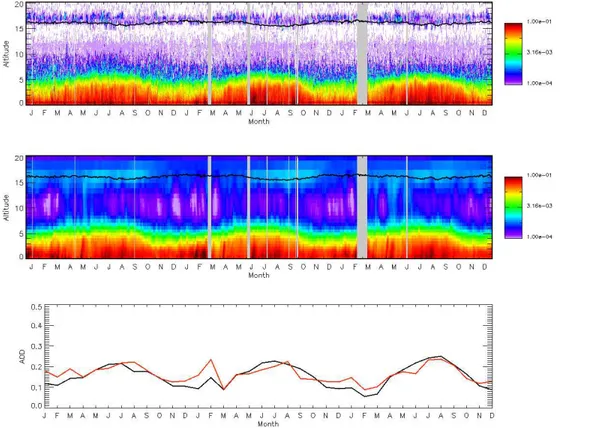
105◦_{E). We constructed a timeseries of CALIOP daily mean aerosol extinction over}

this region from January 2007 to December 2009 (top panel in Fig. 1) by averaging the vertical daily mean aerosol extinctions of all orbit tracks passing through the region defined before. As expected, aerosol extinctions are larger in the lower troposphere, 20

close to pollution sources. The seasonal cycle in aerosol extinction in the lower tro-posphere is similar throughout the 3 yr. An aerosol layer of about 2 km depth is seen at an altitude from 16 to 18 km during the 3 yr of observations. During summer, this very likely corresponds to the aerosol layer described in Vernier et al. (2011a), but we find that the layer remains throughout the winters if one considers a region that 25

(5)

ACPD

12, 2863–2889, 2012

Q. Bourgeois et al.

Title Page

Tables Figures

◭ ◮

Back Close

Full Screen / Esc

Discussion

P

a

per

|

Dis

cussion

P

a

per

|

Discussion

P

a

per

|

Discussio

n

P

a

per

|

Vernier et al. (2011a) used a region extending from 15 to 45◦_{N). Figure 2 depicts a}

lat-itudinal plot of aerosol extinction sampled at the altitude of 16–18 km that shows that the aerosol layer moves northward or southward according to the season. In particular,

the aerosol layer migrates from 20◦_{S in boreal winter to 30}◦_{N in boreal summer and}

matches very well the location of the ITCZ (not shown). This suggests that aerosol 5

precursors and/or aerosols could be transported to the TTL through deep convection associated with the ITCZ (see Sect. 2.2.2 for more details). Once aerosols reach the TTL, their lifetime is likely to increase substantially as hardly any little scavenging can take place due to little concentrations of ice crystals and no liquid phase clouds. Rasch et al. (2008) show that sulfate aerosols during a volcanic period have a lifetime of about 10

2 yr above the tropopause and are likely only removed by sedimentation as ice crystals are inefficient at removing aerosols (Henning et al., 2004).

In the next section, we compare the CALIOP observations with results from the global aerosol-climate ECHAM5.5-HAM2 model and characterize the aerosol layer us-ing a series of model sensitivity simulations.

15

2.2 ECHAM5.5-HAM2 model results

2.2.1 Brief model description

The ECHAM5 (Roeckner et al., 2003) general circulation model (GCM) is coupled with the aerosol module HAM (Stier et al., 2005), here employed in its version ECHAM5.5-HAM2 (Zhang et al., 2012). The aerosol module ECHAM5.5-HAM2 predicts the size distribution 20

and composition (mixing state) of aerosols including sulfate, black carbon (BC), or-ganic carbon (OC), dust and sea salt. The particle size distribution is described by 7 lognormal modes (Vignati et al., 2004) including a sulfate only nucleation mode, three internally mixed hydrophilic modes (Aitken, accumulation and coarse) contain-ing all species, an internally mixed hydrophobic BC/OC mode (Aitken) and two ex-25

(6)

ACPD

12, 2863–2889, 2012

Q. Bourgeois et al.

Title Page

Tables Figures

◭ ◮

Back Close

Full Screen / Esc

Discussion

P

a

per

|

Dis

cussion

P

a

per

|

Discussion

P

a

per

|

Discussio

n

P

a

per

|

phase sulfuric acid condensation sink and ionization rate following the scheme of Kazil and Lovejoy (2007) and implemented in ECHAM5.5-HAM2 as described in Kazil et al. (2010). Integration of the time evolution equation for gas phase H2SO4including

chem-ical production, nucleation and condensation is performed as described in Kokkola et al. (2009). Processes of coagulation and sulfuric acid condensation occur in and/or 5

in between aerosol modes allowing particles to grow and to move from one mode to an-other (Stier et al., 2005). In the model, OC only originates from primary emissions (i.e. without an explicit secondary organic aerosol scheme) which may result in an underes-timate of OC (Kazil et al., 2010). An explicit below-cloud scavenging (Croft et al., 2009) and a semi empirical water uptake schemes were implemented. A double-moment 10

cloud microphysics scheme including prognostic equations for number concentrations of liquid droplets and ice crystals is used (Lin and Leaitch, 1997; Lohmann et al., 1999, 2007, 2008). The in-cloud scavenging scheme makes use of scavenging ratios that are prescribed as a function of aerosol size, aerosol mixing state and cloud type (Stier et al., 2005). In the simulations described in this paper, aerosol scavenging parameters 15

were modified following recommendations from Bourgeois and Bey (2011).

ECMWF meteorological fields (ERA-INTERIM) were used to nudge the model en-abling the representation of large-scale weather systems for specific years. Anthro-pogenic emissions for aerosols are prescribed using the ARCTAS inventory, which is representative of the year 2008 (http://www.cgrer.uiowa.edu/arctas/emission.html). 20

A mix of FLAMBE (Reid et al., 2009) and GFEDv3 (van der Werf et al., 2010) inven-tories were used for biomass burning emissions as reported in Bourgeois and Bey

(2011). A 3-year simulation was performed at a T63L31 resolution (about 1.9×1.9◦ in

the horizontal dimension and 31 vertical levels from the surface up to 10 hPa). Aerosol extinction and AOD are reported at 550 nm.

25

2.2.2 Comparison with CALIOP

(7)

ACPD

12, 2863–2889, 2012

Q. Bourgeois et al.

Title Page

Tables Figures

◭ ◮

Back Close

Full Screen / Esc

Discussion

P

a

per

|

Dis

cussion

P

a

per

|

Discussion

P

a

per

|

Discussio

n

P

a

per

|

for the same region and time period than those provided by CALIOP while Fig. 3 com-pares the observed and simulated annual mean vertical distribution of aerosol extinc-tions over our region of interest. The model reproduces well aerosol extincextinc-tions from the surface to about 8 km but the discrepancy is rather large above 8 km although both the model and the observations similarly show the presence of an enhanced aerosol 5

layer in the TTL (at about 16 km). Observed aerosol extinctions sharply decrease be-tween 8 and 15 km while simulated aerosol extinctions remain at a similar value from 8 to 11 km and slightly increase from 11 to 16 km. In both the observations and the model results, aerosol extinction maximizes at around 16 km, where the model simu-lates the mean tropopause height for the chosen region. The altitude of the observed 10

and simulated aerosol extinction maxima are similar but the model simulates a much broader aerosol layer than the CALIOP retrieval, which shows a finer aerosol layer of

about 2 km thick. The magnitude of these aerosol enhancements are also different with

a mean aerosol extinction of 2.10−4_{and 7.10}−4_km−1_{in the observation and the model,}

respectively. The simulated and observed monthly mean AOD integrated throughout 15

the troposphere show overall good agreement (R2₌₀._{64), but this good agreement}

reflects the fact that the total AOD is largely influenced by the high amount of aerosols found in the planetary boundary layer.

2.2.3 Characterization of the simulated aerosol layer

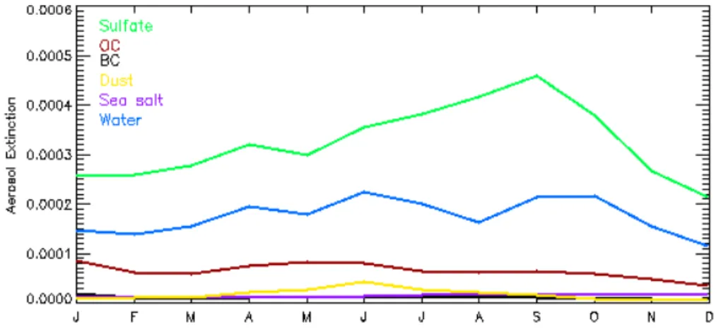
In the following we discuss the monthly mean aerosol extinctions of the aerosol layer 20

for the di_fferent aerosol species and modes simulated in the model (approximated by

volume weighted average of the refractive indices of the individual species). According to the model, sulfate, water and OC contribute 53, 29, and 11 %, respectively, to the aerosol layer extinction, while dust, sea salt, and BC contribute 7 % in total (Fig. 4). The sulfate contribution in the aerosol layer is higher during summer, which likely reflects 25

the ITCZ located over South East Asia where large amounts of anthropogenic SO2

(8)

ACPD

12, 2863–2889, 2012

Q. Bourgeois et al.

Title Page

Tables Figures

◭ ◮

Back Close

Full Screen / Esc

Discussion

P

a

per

|

Dis

cussion

P

a

per

|

Discussion

P

a

per

|

Discussio

n

P

a

per

|

in Southeast Asia (van der Werf et al., 2010). The dust signature is maximum from April to July (about 5 %) and is likely related to dust storms occurring over the Thar desert in Western India during the pre-monsoon season (Dey et al., 2004). The simulated lifetimes of sulfate and OC in the aerosol layer with respect to wet deposition and sedimentation are 116 and 215 days, respectively. Sedimentation contributes 89 and 5

79 % to the sulfate and OC removal, respectively. The remaining 11 and 21 % are due to in-cloud aerosol scavenging.

The annual mean aerosol extinction between 16 and 17.5 km (i.e. at the maximum aerosol extinction) is dominated at 91 % by internally-mixed aerosols in the accumula-tion mode. The internally-mixed coarse mode contributes 8 % and the remaining 1 % is 10

due to other modes such as internally-mixed Aitken mode and externally-mixed modes. In terms of aerosol number concentration, the nucleation mode contributes 99.5 %. This indicates that 0.5 % of the aerosol number concentration (other than aerosols in the nucleation mode) contributes 99 % of the aerosol extinction (91 and 8 % from the internally-mixed accumulation and coarse mode, respectively).

15

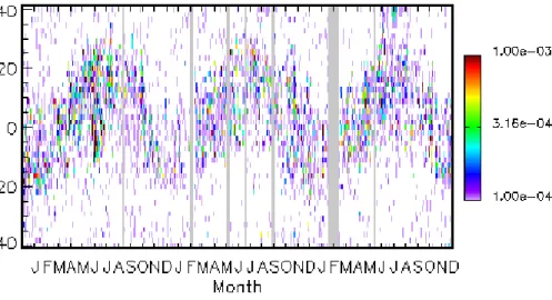
Figure 5 shows the vertical profile of aerosol number concentrations in the nucleation mode. The maximum aerosol number concentration occurs just below the tropopause from 14 to 16 km. The annual mean aerosol number concentration for nucleated aerosols larger than 3 nm (Dp>_{3 nm) in this layer is about 45 000 cm}−3_{(at STP). The}

nucleation aerosol layer between 14 and 16 km is not visible in Fig. 1 because aerosols 20

below 100 nm are not optically active. In order to assess the role of nucleation on the aerosol layer in the TTL, we performed a sensitivity simulation in which nucleation was

turned o_ff. We find that the aerosol number concentration decreases while the mean

aerosol extinction of the aerosol layer increases by about 10 % when nucleation is turned off. This likely reflects the fact that without nucleation, sulfate in the gas phase 25

(9)

ACPD

12, 2863–2889, 2012

Q. Bourgeois et al.

Title Page

Tables Figures

◭ ◮

Back Close

Full Screen / Esc

Discussion

P

a

per

|

Dis

cussion

P

a

per

|

Discussion

P

a

per

|

Discussio

n

P

a

per

|

performed a series of sensitivity simulations in which anthropogenic, biomass burning,

volcanic and DMS emissions were turned o_ffand estimated the relative contributions of

these different emissions by subtracting results from the sensitivity simulations to those from the reference one. These simulations (Fig. 6) show that sulfate in the aerosol

layer is predominantly from SO₂and DMS sources. SO₂ anthropogenic and volcanic

5

emissions account for 35 % each of the total sulfate extinction, SO2 biomass burning

emissions account for 5 %, and DMS terrestrial and marine emissions account for 25 %. Thus, 65 and 35 % of the total sulfate extinction are due to natural and anthropogenic sources, respectively.

In Sect. 2.1, we hypothesis (as many other studies investigating aerosol distribution 10

in the upper troposphere) that the formation of the TTL aerosol layer is at least to some extent driven by deep convection associated with the ITCZ. In the tropics, Hadley cells largely dominate air circulation. Surface air masses from the Southern and Northern Hemisphere converge at the ITCZ near the equator. They rise toward the tropopause near the equator, move slowly poleward, descend toward the surface in the subtrop-15

ics, and flow back toward the Equator near the surface. Over the Asian region, the

ITCZ is located between 5 and 15◦_{S in boreal winter and between 5 and 30}◦_{N in}

boreal summer (Chao, 2000; Lawrence and Lelieveld, 2010). In boreal summer, the ITCZ is located over India (Asian monsoon) where vigorous deep convection reach-ing across the tropopause and up to the lower stratosphere can take place (Gadgil, 20

2003). Fueglistaler et al. (2009) shows that during deep convection event, the main outflow can reach 200 hPa (about 12.5 km near the equator) with rare penetration of the outflow in the TTL. Liu and Zipser (2005) estimated that 1.3 % of the convective air masses reach 14 km and only 0.1 % of them penetrate into the TTL. In a sensitivity simulation in which tracers (including aerosol precursors and aerosols) did not experi-25

(10)

ACPD

12, 2863–2889, 2012

Q. Bourgeois et al.

Title Page

Tables Figures

◭ ◮

Back Close

Full Screen / Esc

Discussion

P

a

per

|

Dis

cussion

P

a

per

|

Discussion

P

a

per

|

Discussio

n

P

a

per

|

3 Discussion

While observed and simulated aerosol extinctions agree quite well in the lower tropo-sphere, there are significant differences in the upper troposphere. In the following we discuss possible reasons related to both the model and the observations for these dif-ferences. Several studies have reported that uncertainties of CALIOP extinction and 5

AOD are likely to be large. For example, a case study reported by Kacenelenbogen et al. (2011) shows that CALIOP version 3 AOD is a factor of two lower than MODIS and AERONET observations in North America. Yu et al. (2010) also reported that CALIOP

AOD observations for different geopolitical regions are lower than MODIS AOD

obser-vations. CALIOP uncertainties are associated with the sensitivity of the instrument, 10

the misclassification of aerosols and clouds, and the determination of the lidar ratio for each type of aerosol (Winker et al., 2009, and references hereafter).

In the particular case of very low aerosol extinctions as found in the TTL, the sen-sitivity threshold (3.10−4_km−1_sr−1 _{Winker et al., 2009) of CALIOP may be the main}

issue. As a result, extinctions in the aerosol layer in the TTL may be too low to be 15

detected, and thus they may be classified as “clear air” (Winker et al., 2009). Chazette et al. (2010) suggested that the lower AOD detection limit of CALIOP is about 0.07 during night and 0.1 during day. Another study (Bourgeois and Bey, 2012) also found that CALIOP significantly underestimates low AOD values in the Northern Hemisphere, in particular below 0.1. Therefore, the sensitivity threshold on the aerosol attenuated 20

backscatter may result in an underestimate of aerosol extinction in the upper tropo-sphere where aerosol extinctions are particularly low. In addition, a maximum uncer-tainty of 30 % for aerosol extinction is associated with the determination of the lidar ratio by the CALIOP algorithm (Omar et al., 2009).

A misclassification of the aerosol type can also induce large errors on the aerosol ex-25

(11)

ACPD

12, 2863–2889, 2012

Q. Bourgeois et al.

Title Page

Tables Figures

◭ ◮

Back Close

Full Screen / Esc

Discussion

P

a

per

|

Dis

cussion

P

a

per

|

Discussion

P

a

per

|

Discussio

n

P

a

per

|

20 sr instead of 40 sr) inducing an underestimate of the AOD by about a factor of 2. An-other source of uncertainty is associated with the cloud-aerosol discrimination (CAD) which is characterized by a confidence value (Liu et al., 2009). Di Pierro et al. (2011) used CALIOP version 2 products and show that dust aerosol can be misclassified as clouds due to their high depolarization ratio. However, Redemann et al. (2011) reported 5

that CALIOP version 3 AOD are similar to or better agree with MODIS observations over oceans than the previous version. Redemann et al. (2011) and Yu et al. (2010) showed that CALIOP observations better reproduce MODIS observations when they used a filter for CALIOP data. For example, Yu et al. (2010) used only “cloud-free”

profiles and aerosol data with a CAD score between−50 and−100 corresponding to

10

a confidence in aerosol data higher than 50 %. In contrast, no screening using CAD

was used in this study because the CAD score of the aerosol layer is between−50 and

0 (not shown), which corresponds to a confidence in aerosol classification lower than 50 %. The low CAD confidence is likely due to the fact that retrieved extinctions in the aerosol layer are very low (close to the detection limit of the instrument).

15

A recent study suggested that overshooting of clean air during convective processes cleans the upper tropical troposphere and lower stratosphere (between 14 and 20 km) in the southern tropic convective season (Vernier et al., 2011b), which is in appar-ent contradiction with our results. Vernier et al. (2011b) used a similar version of

CALIOP product than in our study but applied di_fferent averaging or correction on the

20

data as described in Vernier et al. (2009): First, they averaged nighttime extinctions over large boxes (2◦_longitude

×1◦latitude×200 m in vertical); Second, they process CALIOP data by using a 36–39 km range for the free aerosol background instead of 30–34 km in the CALIOP algorithm; Third, they removed aerosol extinction measure-ments with depolarization ratios larger than 0.05 to avoid a possible misclassification 25

(12)

ACPD

12, 2863–2889, 2012

Q. Bourgeois et al.

Title Page

Tables Figures

◭ ◮

Back Close

Full Screen / Esc

Discussion

P

a

per

|

Dis

cussion

P

a

per

|

Discussion

P

a

per

|

Discussio

n

P

a

per

|

from 0 to 0.05 and from 0.25 to 0.54, respectively. Therefore, averaging high depolar-ization ratios of ice clouds (0.25 to 0.54) with low depolardepolar-ization ratios of aerosols (0 to 0.05) over large grid cells results in depolarization ratios larger than 0.05, which artifi-cially “remove” aerosol layers with weak depolarization ratios from the dataset. This is likely to happen because aerosols and clouds cohabite at the TTL, which makes their 5

distinction difficult. For example, Weigel et al. (2011) observed that aerosols and ice clouds coexist below the TTL in agreement with Thomas et al. (2002) who reported measurements of cirrus clouds there as well. As a matter of fact, the model also sim-ulates a layer of ice crystals between 10 and 16 km just below the aerosol layer (not shown), which possibly confirms the co-existence of aerosols and ice crystals in the 10

TTL. To test the implications of applying a screening based on depolarization ratios on our result, we removed aerosol extinctions with depolarization ratios larger than 0.05 for all profiles above our region of interest but without averaging observations over large grid cells (Fig. 3). This screening results in a decrease of the aerosol extinc-tions throughout the column but the large aerosol extincextinc-tions in the PBL as well as the 15

aerosol enhancement around the TTL remain clearly visible.

Sensitivity model simulations provide additional evidence that the TTL layer is likely composed of aerosols. Two main discrepancies are however remarkable between the model and the observations. First, the aerosol layer in the model is thicker than in the observations, which may be related to the quite large vertical resolution of the model 20

at this altitude (about 1.4 km). Second, aerosol extinctions in the TTL are larger in the model than in the observations which may indicate issues related to sulfate formation, removal or convection in the model. To our knowledge, no measurements of the total number of nucleated particles are available at these altitudes due to extreme mete-orological conditions. Clarke and Kapustin (2002) report a maximum aerosol num-25

ber concentration of 19 000 cm−3 _(Dp_>_{3 nm) at 11 km in the Pacific tropical region}

and a concentration of about 7000 cm−3_(Dp_>_{3 nm) at 12 km. The simulated annual}

mean aerosol number concentration at 11 km in the tropical Pacific region is about

(13)

ACPD

12, 2863–2889, 2012

Q. Bourgeois et al.

Title Page

Tables Figures

◭ ◮

Back Close

Full Screen / Esc

Discussion

P

a

per

|

Dis

cussion

P

a

per

|

Discussion

P

a

per

|

Discussio

n

P

a

per

|

This overestimate was previously reported in Kazil et al. (2010), who suggested that this was not due to a nucleation processes. In addition, the simulated maximum of nucleated aerosol number concentration is located between 14 and 16 km, i.e. higher that the altitude suggested by observations (11 km, even though observations stop at 12 km, Clarke and Kapustin, 2002). This may indicate a too strong convective transport 5

of aerosols and/or aerosol precursors in that region.

SO2Asian anthropogenic emissions could be also too large in our model though our

global and Asian anthropogenic emissions of SO₂ (110 and 40 Tg yr−1_{, respectively)}

agree well with recent estimates such as those provided in Lee et al. (2011). The miss-ing “connection” in CALIOP between aerosols in the lower troposphere and the TTL 10

(Figs. 1 and 3), also discussed in Vernier et al. (2011a), likely results from the pres-ence of convective clouds that mask vertical transport of aerosols. The model actually

simulates large export of sulfate precursors (i.e. SO2 and DMS) toward the tropical

upper troposphere associated with convective processes. These gases further oxidize and their product nucleates to form new particles (e.g., the nucleation aerosol layer be-15

tween 13 and 16 km) or condensate on pre-existing particles, inducing aerosol growth. These particles reach a critical size that matters for extinction once they are in the TTL. This likely explains why no “connection” is seen between the lower troposphere and the upper troposphere in CALIOP.

From these different elements, we conclude that the presence of an aerosol layer in

20

the TTL with a substantial contribution from anthropogenic activities is very likely, even though the amount of aerosols in the TTL aerosol layer is still uncertain.

4 Conclusions and perspectives

CALIOP observations indicate that an aerosol layer remains the entire year in the TTL (at about 16–18 km) and follows the migration of the ITCZ. The confidence for the 25

(14)

ACPD

12, 2863–2889, 2012

Q. Bourgeois et al.

Title Page

Tables Figures

◭ ◮

Back Close

Full Screen / Esc

Discussion

P

a

per

|

Dis

cussion

P

a

per

|

Discussion

P

a

per

|

Discussio

n

P

a

per

|

limit of the instrument. However, particulate depolarization ratios of the particles in the layer are mostly lower than 0.05, which is a typical value for aerosols other than dust.

In order to characterize this aerosol layer, we used the ECHAM5.5-HAM2 model. The model simulates an aerosol layer during the whole year and at the same altitude but the magnitude of the aerosol layer extinction is substantially larger in the model than 5

in observations and the seasonal cycle of the layer is stronger in the model. A sensitiv-ity simulation shows that convection is unambiguously responsible for the formation of the simulated aerosol layer in the TTL. According to the model, sulfate, water and OC contribute 53, 29, and 11 %, respectively, to the aerosol layer extinction, while dust, sea salt, and BC contribute 7 % in total. Extinction due to sulfate aerosols comes from the 10

nucleation and condensation of sulfuric acid, which, in turn, comes at 75 % and 25 %

from the SO2 and DMS oxidation, respectively. SO2 emitted by volcanic and

anthro-pogenic emissions contributes 35 % each to the sulfate extinction in the aerosol layer

while DMS emitted by terrestrial biogenic and marine contributes 25 %. SO₂emitted in

biomass burning emissions contribute 5 %. Therefore, 35 % of the extinction in term of 15

sulfate in the aerosol layer are related to anthropogenic activities while 65 % are due to natural sources. The fast increase in anthropogenic pollution sources in Asia may further increase the proportion due to human activities and, as such, the total aerosol extinction of the TTL aerosol layer, with some possible implications for the chemical and radiative impacts of this aerosol layer. The aerosol layer may have substantial ef-20

fects. As it is mostly composed of sulfate and sulfate aerosols that reflect sunlight, it likely decreases solar radiations absorbed by the atmosphere and induces a cooling of the troposphere over the Southern Asian region. The AOD of the TTL aerosol layer accounts for less than 1 % of the AOD integrated throughout the troposphere (from the surface to 20 km), and therefore the direct effect of aerosols on solar radiation is 25

(15)

ACPD

12, 2863–2889, 2012

Q. Bourgeois et al.

Title Page

Tables Figures

◭ ◮

Back Close

Full Screen / Esc

Discussion

P

a

per

|

Dis

cussion

P

a

per

|

Discussion

P

a

per

|

Discussio

n

P

a

per

|

model indicates that 29 and 42 W m−2 _{are reflected back to space by aerosols and}

clouds, respectively, in the shortwave radiation. Hence, about 6 W m−2 _{(i.e. 14 % of}

42 W m−2_{) are reflected back to space due the cloud formation by aerosols in the TTL.}

From a chemical point of view, sulfate may reduce ozone production in the TTL and in the stratosphere by reacting with ozone precursors (Unger et al., 2006).

5

E_ffects of aerosols, especially sulfate particles, in the TTL have been carefully stud-ied for geoengineering purposes (e.g., Wigley, 2006; Rasch et al., 2008). Some sci-entists and non-scisci-entists proposed to inject sulfate aerosols in the stratosphere to counter global warming associated with increasing greenhouse gases concentrations. However, impacts are still uncertain and more comprehensive studies are needed be-10

fore any definitive conclusion can be reached and the impacts of such propositions as-sessed. The semi-natural aerosol layer over Southeast Asia and the Indian Ocean de-scribed in this study provides great opportunity for better understanding and assessing the chemical and radiative impacts of sulfate aerosols in the upper troposphere. Fur-ther characterization and investigation of the TTL aerosol layer are Fur-therefore needed to 15

reduce remaining uncertainties, especially those related to lidar ratio assignment, cloud aerosol discrimination and measurement threshold of the aerosol attenuated backscat-ter in CALIOP, and to convection strenght, and aerosol formation and deposition in the model.

Acknowledgements. This work was supported by funding from the Swiss National Science 20

Foundation under the grant 200020-124928 and contributes to the EU FP7 IP PEGASOS (FP7-ENV-2010/265148). We thank G. Frontoso, S. Rast and S. Ferrachat for their help with the ECHAM5-HAM code. We acknowledge the CALIOP team for acquiring and processing data as well as the ICARE team for providing and maintaining the computational facilities to store and treat them.

25

References

(16)

ACPD

12, 2863–2889, 2012

Q. Bourgeois et al.

Title Page

Tables Figures

◭ ◮

Back Close

Full Screen / Esc

Discussion

P

a

per

|

Dis

cussion

P

a

per

|

Discussion

P

a

per

|

Discussio

n

P

a

per

|

Res., 105, 26907–26915, 2000. 2872

Bourgeois, Q. and Bey, I.: Pollution transport efficiency toward the Arctic: sensi-tivity to aerosol scavenging and source regions, J. Geophys. Res., 116, D08213, doi:10.1029/2010JD015096, 2011. 2868

Bourgeois, Q. and Bey, I.: Aerosol interannual variability: assessment of AOD retrievals from 5

CALIOP and model comparison, in preparation, 2012. 2872

Chao, W. C.: Multiple quasi equilibria of the ITCZ and the origin of monsoon onset, J. Atmos. Sci., 57, 641–651, 2000. 2871

Chazette, P., Raut, J.-C., Dulac, F., Berthier, S., Kim, S.-W., Royer, P., Sanak, J., Loa ¨ec, S., and Grigaut-Desbrosses, H.: Simultaneous observations of lower tropospheric continen-10

tal aerosols with a ground-based, an airborne, and the spaceborne CALIOP lidar system, J. Geophys. Res., 115, D00H31, doi:10.1029/2009JD012341, 2010. 2872

Clarke, A. D. and Kapustin, V. N.: A pacific aerosol survey. Part I: A decade of data on particle production, transport, evolution, and mixing in the troposphere, J. Atmos. Sci., 59, 363–382, 2002. 2865, 2874, 2875

15

Croft, B., Lohmann, U., Martin, R. V., Stier, P., Wurzler, S., Feichter, J., Posselt, R., and Ferrachat, S.: Aerosol size-dependent below-cloud scavenging by rain and snow in the ECHAM5-HAM, Atmos. Chem. Phys., 9, 4653–4675, doi:10.5194/acp-9-4653-2009, 2009. 2868

Dey, S., Tripathi, S. N., Singh, R. P., and Holben, B. N.: Influence of dust storms on the 20

aerosol optical properties over the Indo–Gangetic Basin, J. Geophys. Res., 109, D20,211, doi:10.1029/2004JD004924, 2004. 2870

Di Pierro, M., Jaegl ´e, L., and Anderson, T. L.: Satellite observations of aerosol transport from East Asia to the Arctic: three case studies, Atmos. Chem. Phys., 11, 2225–2243, doi:10.5194/acp-11-2225-2011, 2011. 2873

25

Froyd, K. D., Murphy, D. M., Sanford, T. J., Thomson, D. S., Wilson, J. C., Pfister, L., and Lait, L.: Aerosol composition of the tropical upper troposphere, Atmos. Chem. Phys., 9, 4363–4385, doi:10.5194/acp-9-4363-2009, 2009. 2865

Fueglistaler, S., Dessler, A. E., Dunkerton, T. J., Folkins, I., Fu, Q., and Mote, P. W.: Tropical tropopause layer, Rev. Geophys., 47, RG1004, doi:10.1029/2008RG000267, 2009. 2871 30

Gadgil, S.: The Indian monsoon and its variability, Annu. Rev. Earth Pl. Sc., 31, 429, 2003. 2871

(17)

ACPD

12, 2863–2889, 2012

Q. Bourgeois et al.

Title Page

Tables Figures

◭ ◮

Back Close

Full Screen / Esc

Discussion

P

a

per

|

Dis

cussion

P

a

per

|

Discussion

P

a

per

|

Discussio

n

P

a

per

|

Aerosol partitioning in natural mixed-phase clouds, Geophys. Res. Lett., 31, L06,101, doi:10.1029/2003GL019025, 2004. 2867

Hu, Y., Winker, D., Vaughan, M., Lin, B., Omar, A., Trepte, C., Flittner, D., Yang, P., Nasiri, S. L., Baum, B., Sun, W., Liu, Z., Wang, Z., Young, S., Stamnes, K., Huang, J., Kuehn, R., and Holz, R.: CALIPSO/CALIOP cloud phase discrimination algorithm, J. Atmos. Ocean. Tech., 5

26, 2293–2309, 2009. 2866, 2873

Kacenelenbogen, M., Vaughan, M. A., Redemann, J., Hoff, R. M., Rogers, R. R., Ferrare, R. A., Russell, P. B., Hostetler, C. A., Hair, J. W., and Holben, B. N.: An accuracy assessment of the CALIOP/CALIPSO version 2/version 3 daytime aerosol extinction product based on a detailed multi-sensor, multi-platform case study, Atmos. Chem. Phys., 11, 3981–4000, 10

doi:10.5194/acp-11-3981-2011, 2011. 2872

Kazil, J. and Lovejoy, E. R.: A semi-analytical method for calculating rates of new sulfate aerosol formation from the gas phase, Atmos. Chem. Phys., 7, 3447–3459, doi:10.5194/acp-7-3447-2007, 2007. 2868

Kazil, J., Stier, P., Zhang, K., Quaas, J., Kinne, S., O’Donnell, D., Rast, S., Esch, M., Fer-15

rachat, S., Lohmann, U., and Feichter, J.: Aerosol nucleation and its role for clouds and Earth’s radiative forcing in the aerosol-climate model ECHAM5-HAM, Atmos. Chem. Phys., 10, 10733–10752, doi:10.5194/acp-10-10733-2010, 2010. 2868, 2875

Kokkola, H., Hommel, R., Kazil, J., Niemeier, U., Partanen, A.-I., Feichter, J., and Timmreck, C.: Aerosol microphysics modules in the framework of the ECHAM5 climate model – intercom-20

parison under stratospheric conditions, Geosci. Model Dev., 2, 97–112, doi:10.5194/gmd-2-97-2009, 2009. 2868

Kulmala, M. and Kerminen, V.-M.: On the formation and growth of atmospheric nanoparticles, Atmos. Res., 90, 132–150, 2008. 2865

Lawrence, M. G. and Lelieveld, J.: Atmospheric pollutant outflow from southern Asia: a review, 25

Atmos. Chem. Phys., 10, 11017–11096, doi:10.5194/acp-10-11017-2010, 2010. 2871 Lee, C., Martin, R. V., van Donkelaar, A., Lee, H., Dickerson, R. R., Hains, J. C., Krotkov, N.,

Richter, A., Vinnikov, K., and Schwab, J. J.: SO₂emissions and lifetimes: estimates from in-verse modeling using in situ and global, space-based (SCIAMACHY and OMI) observations, J. Geophys. Res., 116, D06,304, doi:10.1029/2010JD014758, 2011. 2875

30

(18)

ACPD

12, 2863–2889, 2012

Q. Bourgeois et al.

Title Page

Tables Figures

◭ ◮

Back Close

Full Screen / Esc

Discussion

P

a

per

|

Dis

cussion

P

a

per

|

Discussion

P

a

per

|

Discussio

n

P

a

per

|

Geneva, 328–335, 1997. 2868

Liu, C. and Zipser, E. J.: Global distribution of convection penetrating the tropical tropopause, J. Geophys. Res., 110, D23,104, doi:10.1029/2005JD006063, 2005. 2871

Liu, Z., Vaughan, M., Winker, D., Kittaka, C., Getzewich, B., Kuehn, R., Omar, A., Powell, K., Trepte, C., and Hostetler, C.: The CALIPSO lidar cloud and aerosol discrimination: version 5

2 algorithm and initial assessment of performance, J. Atmos. Ocean. Tech., 26, 1198–1213, 2009. 2866, 2873

Lohmann, U., Feichter, J., Chuang, C. C., and Penner, J. E.: Predicting the number of cloud droplets in the ECHAM GCM, J. Geophys. Res., 104, 9169–9198, 1999. 2868

Lohmann, U., Stier, P., Hoose, C., Ferrachat, S., Kloster, S., Roeckner, E., and Zhang, J.: Cloud 10

microphysics and aerosol indirect effects in the global climate model ECHAM5-HAM, Atmos. Chem. Phys., 7, 3425–3446, doi:10.5194/acp-7-3425-2007, 2007. 2868

Lohmann, U., Spichtinger, P., Jess, S., Peter, T., and Smit, H.: Cirrus cloud formation and ice supersaturated regions in a global model, Environ. Res. Lett., 3, 045022, doi:10.1088/1748-9326/3/4/045022, 2008. 2868

15

Merikanto, J., Spracklen, D. V., Mann, G. W., Pickering, S. J., and Carslaw, K. S.: Impact of nucleation on global CCN, Atmos. Chem. Phys., 9, 8601–8616, doi:10.5194/acp-9-8601-2009, 2009. 2865, 2876

Omar, A., Winker, D. M., Kittaka, C., Vaughan, M. A., Liu, Z., Hu, Y., Trepte, C. R., Rogers, R. R., Ferrare, R. A., Lee, K.-P., Kuehn, R. E., and Hostetler, C. A.: The CALIPSO automated 20

aerosol classification and lidar ratio selection algorithm, J. Atmos. Ocean. Tech., 26, 1994– 2014, 2009. 2866, 2872, 2873

Oo, M. and Holz, R.: Improving the CALIOP aerosol optical depth using combined MODIS-CALIOP observations and MODIS-CALIOP integrated attenuated total color ratio, J. Geophys. Res., 116, D14,201, doi:10.1029/2010JD014894, 2011. 2872

25

Rasch, P. J., Tilmes, S., Turco, R. P., Robock, A., Oman, L., Chen, C., Stenchikov, G. L., and Garcia, R. R.: An overview of geoengineering of climate using stratospheric sulphate aerosols, Phil. Trans. R. Soc. A, 366, 4007–4037, doi:10.1098/rsta.2008.0131, 2008. 2865, 2867, 2877

Redemann, J., Vaughan, M. A., Zhang, Q., Shinozuka, Y., Russell, P. B., Livingston, J. M., 30

(19)

ACPD

12, 2863–2889, 2012

Q. Bourgeois et al.

Title Page

Tables Figures

◭ ◮

Back Close

Full Screen / Esc

Discussion

P

a

per

|

Dis

cussion

P

a

per

|

Discussion

P

a

per

|

Discussio

n

P

a

per

|

Reid, J. S., Hyer, E. J., Prins, E. M., Westphal, D. L., Zhang, J., Wang, J., Christopher, S. A., Curtis, C. A., Schmidt, C. C., Eleuterio, D. P., Richardson, K. A., and Hoffman, J. P.: Global monitoring and forecasting of biomass-burning smoke: description of and lessons from the fire locating and modeling of burning emissions (FLAMBE) program, IEEE J. Sel. Top. Appl., 2, 144–162, 2009. 2868

5

Roeckner, E., B ¨auml, E., Bonaventura, G., Brokopf, L., Esch, R., Giorgetta, M., Hagemann, M., Kirchner, S., Kornblueh, I., Manzini, L., Rhodin, E., Schlese, A., Schulzweida, U., and Tomp-kins, U.: The Atmospheric General Circulation Model ECHAM5: Part 1, Tech. Rep. 349, Max Planck Institute for Meteorology, Hamburg, Germany, 2003. 2867

Stier, P., Feichter, J., Kinne, S., Kloster, S., Vignati, E., Wilson, J., Ganzeveld, L., Tegen, I., 10

Werner, M., Balkanski, Y., Schulz, M., Boucher, O., Minikin, A., and Petzold, A.: The aerosol-climate model ECHAM5-HAM, Atmos. Chem. Phys., 5, 1125–1156, doi:10.5194/acp-5-1125-2005, 2005. 2867, 2868

Thomas, A., Borrmann, S., Kiemle, C., Cairo, F., Volk, M., Beuermann, J., Lepuchov, B., San-tacesaria, V., Matthey, R., Rudakov, V., Yushkov, V., MacKenzie, A. R., and Stefanutti, L.: In 15

situ measurements of background aerosol and subvisible cirrus in the tropical tropopause region, J. Geophys. Res., 107, 4763, doi:10.1029/2001JD001385, 2002. 2874

Twohy, C. H., Clement, C. F., Gandrud, B. W., Weinheimer, A. J., Campos, T. L., Baumgard-ner, D., Brune, W. H., Faloona, I., Sachse, G. W., Vay, S. A., and Tan, D.: Deep convection as a source of new particles in the midlatitude upper troposphere, J. Geophys. Res., 4560, 20

107D21, doi:10.1029/2001JD000323, 2002. 2865

Unger, N., Shindell, D. T., Koch, D. M., Amann, M., Cofala, J., and Streets, D. G.: Influ-ences of man-made emissions and climate changes on tropospheric ozone, methane, and sulfate at 2030 from a broad range of possible futures, J. Geophys. Res., 111, D12,313, doi:10.1029/2005JD006518, 2006. 2877

25

van der Werf, G. R., Randerson, J. T., Giglio, L., Collatz, G. J., Mu, M., Kasibhatla, P. S., Morton, D. C., DeFries, R. S., Jin, Y., and van Leeuwen, T. T.: Global fire emissions and the contribution of deforestation, savanna, forest, agricultural, and peat fires (1997–2009), Atmos. Chem. Phys., 10, 11707–11735, doi:10.5194/acp-10-11707-2010, 2010. 2868, 2870 Vernier, J.-P., Pommereau, J. P., Garnier, A., Pelon, J., Larsen, N., Nielsen, J., Christensen, T., 30

(20)

ACPD

12, 2863–2889, 2012

Q. Bourgeois et al.

Title Page

Tables Figures

◭ ◮

Back Close

Full Screen / Esc

Discussion

P

a

per

|

Dis

cussion

P

a

per

|

Discussion

P

a

per

|

Discussio

n

P

a

per

|

Vernier, J., Thomason, L. W., and Kar, J.: Calipso detection of an asian tropopause aerosol layer, Geophys. Res. Lett., 38, L07,804, doi:10.1029/2010GL046614, 2011a. 2865, 2866, 2867, 2875

Vernier, J.-P., Pommereau, J.-P., Thomason, L. W., Pelon, J., Garnier, A., Deshler, T., Jumelet, J., and Nielsen, J. K.: Overshooting of clean tropospheric air in the tropical 5

lower stratosphere as seen by the CALIPSO lidar, Atmos. Chem. Phys., 11, 9683–9696, doi:10.5194/acp-11-9683-2011, 2011b. 2873

Vignati, E., Wilson, J., and Stier, P.: M7: an efficient size-resolved aerosol microphysics module for large-scale aerosol transport models, J. Geophys. Res., 109, D22,202, doi:10.1029/2003JD004485, 2004. 2867

10

Weigel, R., Borrmann, S., Kazil, J., Minikin, A., Stohl, A., Wilson, J. C., Reeves, J. M., Kunkel, D., de Reus, M., Frey, W., Lovejoy, E. R., Volk, C. M., Viciani, S., D’Amato, F., Schiller, C., Peter, T., Schlager, H., Cairo, F., Law, K. S., Shur, G. N., Belyaev, G. V., and Curtius, J.: In situ observations of new particle formation in the tropical upper troposphere: the role of clouds and the nucleation mechanism, Atmos. Chem. Phys., 11, 9983–10010, doi:10.5194/acp-11-15

9983-2011, 2011. 2865, 2874

Wigley, T. M.: A combined mitigation/geoengineering approach to climate stabilization, Science, 314, 452–454, 2006. 2877

Winker, D. M., Hunt, W. H., and McGill, M. J.: Initial performance assessment of CALIOP, Geophys. Res. Lett., 34, L19,803, doi:10.1029/2007GL030135, 2007. 2866

20

Winker, D. M., Vaughan, M. A., Omar, A., Hu, Y., Powell, K. A., Liu, Z., Hunt, W. H., and Young, S. A.: Overview of the CALIPSO mission and CALIOP data processing algorithms, J. Atmos. Ocean. Tech., 26, 2310–2323, 2009. 2866, 2872

Young, A. and Vaughan, M. A.: The retrieval of profiles of particulate extinction from cloud-aerosol lidar infrared pathfinder satellite observations (calipso) data: algorithm description, 25

J. Atmos. Ocean. Tech., 26, 1105–1119, 2009. 2866

Yu, H., Chin, M., Winker, D. M., Omar, A. H., Liu, Z., Kittaka, C., and Diehl, T.: Global view of aerosol vertical distributions from CALIPSO lidar measurements and GOCART simulations: regional and seasonal variations, J. Geophys. Res., 115, D00H30, doi:10.1029/2009JD013364, 2010. 2872, 2873

30

(21)

ACPD

12, 2863–2889, 2012

Q. Bourgeois et al.

Title Page

Tables Figures

◭ ◮

Back Close

Full Screen / Esc

Discussion

P

a

per

|

Dis

cussion

P

a

per

|

Discussion

P

a

per

|

Discussio

n

P

a

per

|

(22)

ACPD

12, 2863–2889, 2012

Q. Bourgeois et al.

Title Page

Tables Figures

◭ ◮

Back Close

Full Screen / Esc

Discussion

P

a

per

|

Dis

cussion

P

a

per

|

Discussion

P

a

per

|

Discussio

n

P

a

per

|

(23)

ACPD

12, 2863–2889, 2012

Q. Bourgeois et al.

Title Page

Tables Figures

◭ ◮

Back Close

Full Screen / Esc

Discussion

P

a

per

|

Dis

cussion

P

a

per

|

Discussion

P

a

per

|

Discussio

n

P

a

per

|

(24)

ACPD

12, 2863–2889, 2012

Q. Bourgeois et al.

Title Page

Tables Figures

◭ ◮

Back Close

Full Screen / Esc

Discussion

P

a

per

|

Dis

cussion

P

a

per

|

Discussion

P

a

per

|

Discussio

n

P

a

per

|

Fig. 4.Monthly mean aerosol extinction (km−1

(25)

ACPD

12, 2863–2889, 2012

Q. Bourgeois et al.

Title Page

Tables Figures

◭ ◮

Back Close

Full Screen / Esc

Discussion

P

a

per

|

Dis

cussion

P

a

per

|

Discussion

P

a

per

|

Discussio

n

P

a

per

|

(26)

ACPD

12, 2863–2889, 2012

Q. Bourgeois et al.

Title Page

Tables Figures

◭ ◮

Back Close

Full Screen / Esc

Discussion

P

a

per

|

Dis

cussion

P

a

per

|

Discussion

P

a

per

|

Discussio

n

P

a

per

|

(27)

ACPD

12, 2863–2889, 2012

Q. Bourgeois et al.

Title Page

Tables Figures

◭ ◮

Back Close

Full Screen / Esc

Discussion

P

a

per

|

Dis

cussion

P

a

per

|

Discussion

P

a

per

|

Discussio

n

P

a

per

|